| Issue |
A&A
Volume 581, September 2015
|
|
|---|---|---|
| Article Number | A88 | |
| Number of page(s) | 8 | |
| Section | Stellar atmospheres | |
| DOI | https://doi.org/10.1051/0004-6361/201526586 | |
| Published online | 10 September 2015 | |
The origin of fluorine: abundances in AGB carbon stars revisited
1
Dpto. Física Teórica y del Cosmos, Universidad de Granada,
18071
Granada,
Spain
e-mail:
This email address is being protected from spambots. You need JavaScript enabled to view it.
2
Observatório Nacional, Rua General José Cristino, 77, 20921-400 São
Critovão, Rio de
Janeiro, RJ,
Brazil
3
INAF, Osservatorio Astronomico di Collurania,
64100
Teramo,
Italy
4
INFN Sezione Napoli, Napoli, Italy
5
Laboratoire Lagrange, Université Côte d’Azur, Observatoire de la
Côte d’Azur, CNRS, CS
34229, 06304
Nice Cedex 4,
France
Received: 22 May 2015
Accepted: 9 July 2015
Abstract
Context. Revised spectroscopic parameters for the HF molecule and a new CN line list in the 2.3 μm region have recently become available, facilitating a revision of the F content in asymptotic giant branch (AGB) stars.
Aims. AGB carbon stars are the only observationally confirmed sources of fluorine. Currently, there is no consensus on the relevance of AGB stars in its Galactic chemical evolution. The aim of this article is to better constrain the contribution of these stars with a more accurate estimate of their fluorine abundances.
Methods. Using new spectroscopic tools and local thermodynamical equilibrium spectral synthesis, we redetermine fluorine abundances from several HF lines in the K-band in a sample of Galactic and extragalactic AGB carbon stars of spectral types N, J, and SC, spanning a wide range of metallicities.
Results. On average, the new derived fluorine abundances are systematically lower by 0.33 dex with respect to previous determinations. This may derive from a combination of the lower excitation energies of the HF lines and the larger macroturbulence parameters used here as well as from the new adopted CN line list. Yet, theoretical nucleosynthesis models in AGB stars agree with the new fluorine determinations at solar metallicities. At low metallicities, an agreement between theory and observations can be found by handling the radiative/convective interface at the base of the convective envelope in a different way.
Conclusions. New fluorine spectroscopic measurements agree with theoretical models at low and at solar metallicity. Despite this, complementary sources are needed to explain its observed abundance in the solar neighbourhood.
Key words: stars: AGB and post-AGB / stars: abundances / nuclear reactions, nucleosynthesis, abundances
© ESO, 2015
1. Introduction
Fluorine has only one stable isotope, 19F, yet fragile and easily destroyed in stellar interiors by proton, neutron, and alpha particle capture reactions. Major fluorine destruction channels are 19F(p,α)16O and 19F(α,p)22Ne reactions. Thus, any production mechanism also has to enable 19F to escape from the hot stellar interiors after its production. This makes fluorine a useful tracer of the physical conditions prevailing in stellar interiors. Fluorine is thought to be produced in several scenarios: (i) gravitational supernovae through the neutrino spallation process; (ii) low and intermediate mass (M ≤ 7 M⊙) asymptotic giant branch (AGB) stars1 during the He-burning thermal pulses (TP) and the subsequent third dredge-up (TDU) episodes; (iii) Wolf-Rayet (WR) stars in the hydrostatic He-burning phase and, even; (iv) during white dwarfs mergers (see e.g. Woosley et al. 1990; Forestini et al. 1992; Meynet & Arnould 2000; Longland et al. 2011). To date, proof of this production has only been found in AGB stars (e.g. Jorissen et al. 1992; Werner et al. 2005; Otsuka et al. 2008; Abia et al. 2010; Lucatello et al. 2011). The origin of this element is therefore still rather uncertain and contributions from the above mentioned sources seem to be necessary when comparing Galactic chemical evolution (GCE) model predictions (Renda et al. 2004; Kobayashi et al. 2011) to the evolution inferred from observations in Galactic field dwarf and giant stars (Recio-Blanco et al. 2012; Jönsson et al. 2014a).
Accurate determinations of F abundances are needed to determine the relative role of the above proposed sources of fluorine and, in particular, of AGB stars. Fluorine abundances are usually determined in cool dwarfs and giants from ro-vibrational HF lines at 2.3 μm. This spectral region, unfortunately, is placed in a region with a lot of telluric lines that can be difficult to be removed. In many cases, this prevents the use of several HF lines to determine the F abundance in a given star. The most used line is the R9 λ 2.3358 μm HF line, which is marginally affected by blends and telluric lines (Abia et al. 2009; de Laverny & Recio-Blanco 2013). Jorissen et al. (1992) first used this line and other secondary HF lines to derive F abundances in AGB stars of both oxygen- and carbon-rich types2 showing indeed that AGB stars present large fluorine enhancements. Most recently, Abia et al. (2009, 2010) revisited this pioneering analysis using a new grid of atmosphere models for AGB carbon stars and an updated molecular and atomic line lists in the 2.3 μm region. Yet, they found significant F enhancements but systematically lower than those in Jorissen et al. (1992). Nevertheless, the new F enhancements are in a global agreement with nucleosynthesis calculations of low-mass AGB stars with near solar metallicity (Cristallo et al. 2011), although at lower metallicities models predict larger enhancements than observed (Abia et al. 2011; Lucatello et al. 2011). The mentioned abundance analyses in AGB stars, however, were performed using HF line excitation energies inconsistent with the partition functions adopted in the spectral synthesis. In fact, Abia et al. (2009, 2010, 2011) used the Turbospectrumv10.2 radiative transfer code (Plez 2012), which adopts partition functions from Sauval & Tatum (1984). However, the HF line excitation energies used in those works were from Jorissen et al. (1992, in turn from Tipping, priv. comm.), are 0.25 eV higher than the correct values if using the Sauval & Tatum (1984)’s partition functions. As mentioned by Jönsson et al. (2014b), the 0.25 eV different adopted excitation energies comes from the fact that the Tipping list uses the dissociation energy of the energy potential, and not, like Sauval & Tatum (1984), the true energy required for dissociation. The former is higher because of the zero point of the energy of the lowest vibrational level. The difference is exactly 0.25 eV for HF (Zemke et al. 1991). Recently, Jönsson et al. (2014b) presented a complete and comprehensive calculation of the excitation energies and transition probabilities for the HF molecule in the K- and L-bands. The computed HF molecular parameters agree nicely with the new list of experimental molecular parameters delivered by the HITRAN database (see Rothman et al. 2013, for details on this database). As a consequence, and according to the simple curve of growth, F abundances derived with consistent partition functions would be lower by an amount ~θΔχ, where θ = 5040 /Teff and Δχ = 0.25 eV.
Very recently, a new solar F abundance has been determined from the analysis of a sunspot spectrum (Maiorca et al. 2014). The new solar abundance, log ϵ(F) = 4.40 ± 0.253, is significantly lower that the previous commonly adopted value 4.56 ± 0.30 (although it is in agreement within the error bars, Asplund et al. 2009) and it is in a very good agreement with the meteoritic value, 4.46 ± 0.06 (Lodders et al. 2009). Finally, Hedrosa et al. (2013) provided a new CN line list that might affect the fluorine abundance determination in carbon-rich stars from the 2.3 μm region. As a consequence, in light of the new molecular parameters and solar fluorine abundance, a re-determination of fluorine abundances in AGB stars is needed to evaluate their actual contribution to the Galactic fluorine inventory. This is the aim of the present work.
In Sect. 2, we describe the observations and the new spectroscopic tools used for the re-determination of the fluorine abundances in AGB carbon stars. Section 3 shows our results, while we present our conclusions in Sect. 4.
2. Analysis and results
The stars studied here are the same than those analysed in Abia et al. (2010) and Abia et al. (2011), corresponding to Galactic and extragalactic AGB carbon star samples, respectively (thereafter Papers I and II). The extragalactic stars belong to the Carina dwarf galaxy (two stars) and the Magellanic Clouds (two stars in the SMC and one star in the LMC). Details about the observations, data reduction procedures, and quality of the final spectra can be found in these previously published works. The redetermination of fluorine abundances in these stars has been made using the spectral synthesis method in local thermodynamical equilibrium (LTE) with the new version (v14.1) of the Turbospectrum code. Theoretical spectra were computed using the same atmospheric parameters (Teff, log g, [Fe/H]4, and microturbulence) as in Papers I and II (see those for details), the only difference being the molecular line lists used here (however see below about changes in the macroturbulence parameter). As noted before, the new HF line excitation energies from Jönsson et al. (2014b) are now consistent with the partition functions adopted in the Turbospectrum code. The immediate consequence of the systematically 0.25 eV lower excitation energies is that in AGB carbon stars most of the HF lines in the 2.3 μm region are saturated (log (Wλ/λ) ≥ −4.0), even for moderate (solar) fluorine abundances. This makes the HF lines more sensitive to the microturbulence parameter (see Fig. 1) and, as a consequence, the total uncertainty in the derived F abundances would be larger. For instance a change in the microturbulence by ± 0.2 km s-1 may change the F abundance derived up to ∓0.15 dex.
Updates in the molecular line lists in the 2.3 μm region has been made. In particular, we have included the contribution from the HCN molecule (H12CN/H13CN) according to the computations by Harris et al. (2003). We also corrected the wavelengths and intensities of some H2O and OH lines in this spectral region following the new HITRAN database release. Nevertheless, because of the carbon-rich nature of our stars, the contribution to the global spectrum of these two later molecules is minimal. This is not the case, however, for the HCN molecule, which contributes somewhat by introducing a global extra-absorption (veil) that might diminish the spectral continuum up to ~2−3%. Also, a significant change with respect to the line lists used in previous works is the updated CN line list in this spectral region. Details on how this CN list was computed can be found in Hedrosa et al. (2013). The new CN line list has an impact on the global fitting of the observed spectra: theoretical fits are improved for most of the stars. For several stars, the C/O ratio corresponding to the best fit to the observed spectrum needed to be revised when compared to the derived value in Papers I and II (compare Table 1 in these works with Table 2 here). Also, for the stars R Lep and SS Vir in Paper I we could not obtain a good fit to their spectra and, thus, these stars were discarded from the analysis. On the contrary, we now find a good global fit to the spectrum of the extragalactic carbon star LMC TRM88, and determine its F abundance (previously we had just derived an upper limit F abundance for this star, see Table 1 in Paper II). The new CN line list also affects the HF lines in different ways: while the R9 line still remains almost unblended, the R22, R17, and R16 HF lines, which were used in Abia et al. (2010, see their Table 2), are now quite blended with CN features (see Fig. 1) and have to be considered as secondary F abundance indicators. On the contrary, the R23, R15, and R14 HF lines show less blending than before with CN lines and complement the R9 line as main fluorine indicators.
Variations (new-old) in the F abundance derived (in dex) from some HF lines due to the combined effect of the new χ’s and CN molecular list for specific atmosphere parameters.
Figure 1 shows examples of synthetic fits compared to observed spectra of the stars TX Psc and UU Aur. The impact of the new excitation energies of the HF lines, micro- and macroturbulence parameters and that of the new CN line list used in the 2.3 μm region on the derivation of the F abundance can clearly be appreciated.
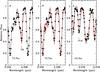 |
Fig. 1 Examples of synthetic fits (continuous and dotted lines) to the observed spectra (dots) for typical AGB carbon stars in the region of some HF lines. Panel a) (left): black line is the best fit to the R9 HF line in TX Psc (log ϵ(F) = 4.7,ξ = 2.2 km s-1 and Γ = 13 km s-1); red line is a fit assuming a 0.45 dex larger F abundance to show the effect of a F abundance variation similar to the total error estimated on [F/H] (see text); and the dotted red line shows the corresponding synthetic spectrum adopting the previously wrong lower excitation energy for this line, χ = 0.48 eV. Panel b) (centre): black line the same as case a; red line is a synthetic spectrum adopting a lower macroturbulence parameter Γ = 11 km s-1; and the dotted red line adopts a lower microturbulence, ξ = 1.8 km s-1 than in case a, respectively. Panel c) (right): effect of our new CN line list (black line) compared with the older line list (red line) on the fit to the R16 HF line at λ ~ 2.2778μm in the carbon star UU Aur. |
Fluorine abundances and element ratios.
2.1. The fluorine abundance in the Sun and Arcturus
Solar abundances are used as a zero point for all the abundance studies. Also, Arcturus is a benchmark star in abundance analyses of cool giants. To make this analysis as consistent as possible, we redetermined the F abundance in these two reference stars using the above new molecular parameters and line lists. For the Sun, we used the sunspot umbra spectra in the region 1.16 to 2.5 μm by Wallace et al. (2001), and followed the same procedure as in Maiorca et al. (2014) to estimate the effective temperature of the atmospheric model that is most compatible with the sunspot umbra spectrum. We used weak and moderate intensity OH lines at 1.5 μm together with some CO lines at 2.3 μm. Atomic lines of the metals present in these spectral regions cannot be used for this purpose since most of them are affected by Zeeman splitting. This is not the case for the CO and OH molecular lines, nor for the HF lines because the corresponding vibro-rotational transitions have no spin nor orbital momentum, which means there is a very weak coupling between the rotational momentum and magnetic field. In fact, by using a simple Milne atmosphere model and a vertical magnetic field, we checked that these molecular lines would only be affected by Zeeman splitting for magnetic fields larger than ~106 G, an intensity much larger than that observed in the sunspots. We estimated a value Teff = 3800 K from the best fit to the CO and OH lines in the sunspot spectrum. Thus we used a MARCS model atmosphere with parameters Teff/ log g/ [ Fe/H ] = 3800/4.44/0.0 interpolated from a grid of atmosphere models (Gustafsson et al. 2008)5. Similar to Maiorca et al. (2014), we found that the cores of the stronger CO and of some OH lines were not so well matched. This difficulty has already been reported in the analysis of the infrared spectra of many K giants with Teff similar to that we estimated in the sunspot (e.g. Ryde et al. 2002; Tsuji 2008, 2009), suggesting that the CO fundamental lines cannot only be interpreted with a photospheric model. These lines show an excess absorption (log Wλ/λ ≥ −4.75), which is probably non-photospheric in origin, indicating that the structure of the hydrostatic atmosphere does not properly describe that of the sunspots6. Maiorca et al. (2014) arrived at the same conclusion, nevertheless, they estimated a Teff = 4250 K as the best value matching both the OH and CO lines in the sunspot spectrum. Nevertheless, we derive log ϵ(F) = 4.37 ± 0.04 in the Sun from 10 HF lines, in agreement with the value estimated by Maiorca et al. (2014) and with the meteoritic abundance (Lodders et al. 2009). The uncertainty in this value is mainly determined by the error in the temperature estimate of the sunspot spectrum. Maiorca et al. (2014) quoted about 0.25 dex for this error, which we also adopt here. In the following, we use our derived F abundance as the reference value for the Sun.
For Arcturus, we used the electronic version of the infrared atlas spectrum by Hinkle et al. (1995) and the atmosphere parameters from Ryde et al. (2009). We obtain a fluorine abundance of log ϵ(F) = 3.78 ± 0.03 from the analysis of the R7, R9 and R12 HF lines. This value is also in excellent agreement with that obtained by Jönsson et al. (2014a, b), the latter from the analysis of some HF lines at 12.2 μm.
2.2. Fluorine abundances in AGB carbon stars
Table 2 (second column) shows the fluorine abundances redetermined in the sample of Galactic and extragalactic AGB carbon stars of different spectral types. For each star we report the number of HF lines used (between parenthesis) and the corresponding dispersion when more than a single line was used. Table 2 also shows (third column) the difference in the F abundance derived with respect to those in Papers I and II. The mean difference is −0.33 ± 0.17 dex, i.e. the abundances derived here are on average systematically lower by this amount. Note that for many stars the reduction in the F abundance is different from that applying just the correction factor ~5040 /TeffΔχ (see Table 1). The reason is twofold: a) the impact of the new CN line list and; b) the use here of larger macroturbulence velocities (Γ) with respect to those used in Papers I and II. The new CN line list and partition functions affects the HF lines in a different manner, depending on the actual C/O ratio and the metallicity of the star (see Table 1). The former effect depends on the blending of a specific HF line with CN lines (see Fig. 1) which are, in any case, no larger than ~± 0.20 dex. On the other hand, because of the use of new molecular line lists (mainly CN), we realised that the 2.3 μm spectral region is better fitted using a macroturbulence parameter in the range 13−14 km s-1 (see Fig. 1), instead of 11−12 km s-1 adopted in Papers I and II. This might increase the fluorine abundance as much as 0.25 dex, partially compensating the systematic decrease of the F abundances because of the lower χ values. In summary, the F abundances derived here differ from the previous values by an amount, which is different star by star, depending on the combined effect of the lower χ values, the higher Γ parameters, and the blending with CN lines, in this order of relevance.
The total uncertainty in the abundance determination can be determined from the dependence of the fluorine abundance on the stellar atmospheric parameters; this dependence is rather similar for all the HF lines, being the uncertainty in Teff, ξ, Γ and the C/O ratio the main sources of error. A detailed discussion on the error sources and their impact in the final F abundance can be found in Abia et al. (2009). Also a discussion on the uncertainties in the derivation of the stellar metallicity [Fe/H] and s-element abundances can be found in Abia et al. (2001, 2002); de Laverny et al. (2006), and Abia et al. (2008). Concerning F, the quadratic addition of all these sources of error gives a typical uncertainty of ±0.40 dex, together with the uncertainty of the continuum position and the dispersion in the F abundance when derived from several lines, a conservative total error would be ±0.45 dex. This value does not include possible systematic errors as those as in the model atmospheres structure and/or non-LTE effects. However, the uncertainty in the abundance ratio between F and any other element would be lower than this value, since some of the above uncertainties cancel out when deriving the abundance ratio. Note, however, that the new [F/Fe] ratios in many stars (Col. 5 in Table 2), do not differ significantly from the previous ratios because the reduction of the solar F abundance by 0.19 dex (see previous section).
3. Discussion
The main consequence of the redetermined F abundances is that they are systematically lower than those in previous determinations, in particular, for carbon stars of near solar metallicity. As it can be seen in Table 2, normal (N-type) carbon stars show only moderate F enhancements ([F/Fe]); the largest enhancements are now close to ~1 dex but are only observed in one SC-type star (WZ Cas) and some of the metal-poor N-type stars in Carina and the Magellanic Clouds. On the other hand, J-type carbon stars show no F enhancements or, in some cases, even depletions (RY Dra and Y Cvn, see Table 2). We confirm, therefore, the results of Paper I concerning the [F/Fe] ratios in AGB carbon stars of different spectral types. These new enhancements can still be accounted for by current low-mass TP-AGB nucleosynthesis models (see below).
We compare the revised F abundances with theoretical models computed with the FUNS evolutionary code (Straniero et al. 2006; Cristallo et al. 2009). Those models are available on-line on the web pages of the FRUITY7 database, which includes stars with initial masses 1.3 ≤ M/M⊙ ≤ 6.0 and metallicities −2.15 ≤ [Fe/H] ≤ +0.15 (Cristallo et al. 2011, 2015b). Those models are calculated by coupling the physical evolution of the structure with a nuclear network including all chemical species, from hydrogen up to Pb-Bi (at the termination of the s-process path). Thus, no post-process techniques are used. In FRUITY models, a thin 13C pocket forms after each TDU episode. The mass extension of the pockets decreases along the AGB, thus making the first pockets the most significant for the on-going s-process nucleosynthesis. The mass-loss rate is calibrated on the observed mass-loss period relation found in Galactic AGB stars (see Straniero et al. 2006, and references therein). To properly follow the physical behaviour of the most external layers, low-temperature C and N enhanced molecular opacities are used (Cristallo et al. 2007). In fact, if the convective envelope becomes C-rich (i.e. C/O > 1), C-bearing molecules form, which largely contributes to the opacity (more than O-bearing molecules). Thus, the structure becomes more opaque to photons and the external layers expand and cool. This implies an increased mass-loss rate. With respect to previously published FRUITY low-mass AGB star yields (Cristallo et al. 2011), we find lower F surface abundances due to a revision in the opacity treatment of the sub-atmospheric region (Cristallo et al. 2015b). We confirm previous calculations (Lugaro et al. 2004; Karakas 2010) showing that the stellar mass range for F production peaks around 1.5−2.5 M⊙ for all Z, showing a small dependence on the metallicity. This implies that very large surface [F/Fe] ratios are predicted for decreasing metallicities. Net fluorine yields from IMS stars are lower than their low-mass counterparts, but indeed have a stronger dependence on the metallicity. In fact, in our low Z IMS models the 19F(p,α)16O and 19F(α,p)22Ne reactions are more efficiently activated, both leading to a net fluorine destruction. In any case, however, the IMS contribution to the fluorine is negligible because these stars experience a definitely less efficient TDU (see Cristallo et al. 2015b).
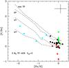 |
Fig. 2 [F/Fe] vs. [Fe/H] in the stars analysed. Circles data points are: black, N-type Galactic carbon stars; red, J-type; green, SC-type and blue, extragalactic N-type carbon stars. Dashed lines represent theoretical predictions for a non-rotating 2 M⊙ TP-AGB star at different TPs, according to Cristallo et al. (2015b). A typical error bar is indicated. |
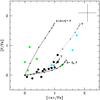 |
Fig. 3 Observed fluorine vs. average s-element enhancements compared with theoretical predictions. Circles symbols are as in Fig. 2. Solid lines are the predictions for a non-rotating 2 M⊙ TP-AGB with metallicities (labelled) mimicking those of our stellar sample assuming the standard 13C-pocket, according to Cristallo et al. (2015b; labelled F, FRUITY). Dotted line is the prediction for a non-rotating 1.3 M⊙ metal-poor model for the same metallicities in the hypothesis of a larger 13C-pocket (labelled T, Tail; see text). Small open squares in these lines mark the values predicted at different TPs. J-type AGB carbon stars have been excluded because they usually do not show s-element enhancements (Abia & Isern 2000). Typical uncertainties are shown. See text for details. |
Figure 2 shows the [F/Fe] ratios derived in our stars versus the stellar metallicity. The different dots refer to the different spectral types carbon stars in the Galaxy (see figure caption). Blue dots are the extragalactic metal-poor carbon stars belonging to the satellite galaxies. From this figure, it is evident that J-type stars tend to be F-poor objects compared to the normal N-type (black dots) carbon stars. Moreover, there is a hint that SC-type stars show, on average, larger F enhancements with respect to N-type stars. With the present analysis, we confirm what we found in Paper I in this respect, however, the origin of SC- and J-type stars is still unknown. There is evidence that they are outside the classical spectral evolution M-MS-S-C(N) along the AGB phase, which is thought to be a consequence of the progressive carbon enrichment of the stellar envelope because of TDU episodes8. Nevertheless, the small number of J- and SC-type stars studied prevent us to reach a definite conclusion. Figure 2 demonstrates that Galactic N-type stars with slightly lower [Fe/H] present larger [F/Fe]. This trend is confirmed for the extragalactic AGB carbon stars (blue dots), which show definitely larger fluorine overabundances, thus confirming the results of Paper II. Dashed lines in Fig. 2 are the predicted [F/Fe] ratios as a function of the metallicity for a typical non-rotating 2 M⊙ AGB star at different TPs (as labelled). It can be seen that observed and predicted [F/Fe] ratios agree well within observational errors. Furthermore, the predicted C/O ratios in the envelope at the observed metallicity of the stars agree with the corresponding observed F enhancement. For instance, in the FRUITY database models with [ Fe/H ] ~ 0.0,−1.1,−2.1 (or Z = 0.014,10-3 and 10-4, respectively) at the 3rd TP, the predicted ratios are C/O ~ 1.1,2.0 and 15, respectively. These C/O ratios are compatible with those measured in our sample at those metallicities (see Table 2). In brief, we confirm here the predicted dependence of the F production with the metallicity (e.g. Lugaro et al. 2004; Cristallo et al. 2011; Fishlock et al. 2014).
A correlation between the F and the s-element overabundance is expected if a large enough 13C pocket forms after each TDU episode. This correlation comes from the 15N production in the radiative 13C pocket, which is the site where the s-process main component is built up (see Paper I for details). Figure 3 shows the new [F/Fe] ratios vs. the observed average s-element enhancement (Abia et al. 2002, 2008; de Laverny et al. 2006). For the solar-like metallicity N-type carbon stars (black dots), F and s-element overabundances clearly correlate. This trend seems to hold for metal-poor extragalactic carbon stars (blue dots) as well, with the largest fluorine overabundances corresponding to the most s-process rich stars. In Fig. 3 we compare observations with FRUITY models having two different (M, Z) combinations, i.e. initial mass M = 2 M⊙ with [ Fe/H ] = 0 and M = 1.3 M⊙ with [ Fe/H ] = −1.67. Both curves start from FDU abundances (solid curves). The two metallicities are representative of Galactic and extragalactic carbon stars, respectively. At low Z we choose a lower initial mass to be consistent with the bolometric magnitudes of the observed stars (−4.3 <Mbol< −5.3). At solar metallicity, observations (excluding most of SC stars) and theory (the two lower curves in Fig. 3) agree nicely. At low Z (upper continuos line in Fig. 3), instead, we highlight a clear disagreement; the models show too large 19F abundances for a fixed s-process enrichment (see the discussion in Abia et al. 2011). A similar apparent deficiency of F abundances for a given s-element enhancement has also been found in the Galactic Carbon Enhanced Metal-Poor stars (CEMP), which are believed to have been polluted by mass-transfer from a former AGB star in a binary system (e.g. Lucatello et al. 2011). We test whether the inclusion of rotation might alleviate this problem by modifying the 19F surface distributions in our models (see Piersanti et al. 2013). The main fluorine production channel starts with the neutrons released by the 13C(α,n)16O reaction and proceeds through the nuclear chain 14N(n,p)14C(α,γ)18O(p,α)15N (α,γ)19F (see Cristallo et al. 2014, and references therein). The main effect of mixing induced by rotation is to dilute 14N within the 13C-pocket. Thus, more neutrons are captured by 14N, feeding the nuclear path leading to 19F production. This also has important consequences for the on-going s-process nucleosynthesis, which has less efficient results, depending on the initial rotation velocity (14N is in fact the major neutron poison of the s-process). Thus, rotation leads to slightly larger fluorine surface abundances and to a definitely lower s-process efficiency. We conclude, therefore, that this physical process cannot be considered as a potential candidate to solve the fluorine discrepancy between theory and observations at low metallicities. A possible way to solve this discrepancy is to obtain larger s-process enhancements for a fixed dredged-up mass. Cristallo et al. (2015b) recently demonstrated that a different treatment of the inner boundary of the extra-mixed region at the base of the convective envelope during a TDU may lead to appreciable differences in the surface s-process distribution. In particular, those authors found that allowing the partial mixing to work below the formal Schwarzschild convective boundary down to the layer where the convective velocity is 1011 times lower, a net increase of s-process abundances can be obtained. This derives from the fact that 13C pockets are larger than those obtained in standard FRUITY models (in which the lower boundary is fixed at 2 pressure scale heights from the formal border of the convective envelope). In Fig. 3 we report two models with the same combination of mass and metallicity as the FRUITY models already discussed, but with the aforedescribed different mixing treatment at the base of the convective envelope (dotted lines in Fig. 3). At solar-like metallicity, we find a slight increase in the fluorine surface overabundances, which does not compromise the agreeement with observations. At low Z, instead, we notice a large fluorine reduction for a fixed s-process surface enhancement. This leads to a reasonable fit to extra-galactic carbon stars. Thus, we conclude that larger 13C pockets than those characterising FRUITY models are needed to fit fluorine abundances in the metal-poor extra-galactic carbon stars. This further strengthens similar conclusions already reached in the study of s-process rich stars belonging to open clusters (Maiorca et al. 2012; Trippella et al. 2014) as well as in the isotopic analysis of pre-solar SiC grains (Liu et al. 2014, 2015). In any case, SC-type carbon stars marginally agree with theoretical models, however, the evolutionary status of these objects is not well understood.
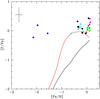 |
Fig. 4 [F/Fe] vs. [Fe/H] observed in Galactic field dwarfs and giants, and open cluster stars compared with the predicted evolution from our GCE model for the solar neighbourhood, including only fluorine production from AGB stars. Black line: yields from Cristallo et al. (2015a); Red line: yields from Karakas (2010). The observed ratios (circles) are from Recio-Blanco et al. (2012; black), Li et al. (2013; blue), Maiorca et al. (2014; green), Jönsson et al. (2014b; cyan) and Nault & Pilachowski (2013; magenta). A typical error bar is shown. See text for details. |
3.1. The contribution of AGB stars to the fluorine abundance in the solar neighbourhood
As mentioned in Sect. 1, the real contribution of AGB stars to the F inventory in the solar neighbourhood is still a matter of debate (Jönsson et al. 2014a). The present downward revision of the F overabundances observed in AGB stars and new model predictions reopen this issue. To shed light on this problem, we have computed a simple Galactic Chemical Evolution (GCE) model (Cristallo et al. 2015a) used recently to study the solar system s-only distribution (i.e. of those isotopes uniquely synthesised by AGB stars). This GCE model accounts for all the constraints currently observed in the solar neighbourhood and at the epoch of the solar system formation (Boissier & Prantzos 1999). By using this code, we have calculated the [F/Fe] vs. [Fe/H] evolution including only the F contribution from AGB stars. Figure 4 shows the computed evolution (black line) compared to the observed one inferred from Galactic unevolved field dwarf and giant stars and open cluster stars (see caption of Fig. 4 for the references9). It is evident that the AGB contribution to F is not enough to account for the observed abundance of this element in the solar system: the GCE model predicts a factor ~3 lower [F/Fe] ratio than observed at [ Fe/H ] ~ 0.0. We have also computed the evolution using the F yields obtained with the STROMLO stellar evolutionary code (see e.g. Karakas 2010, red line). From Fig. 4, it is also evident that the GCE model produces quite different results when using different 19F yield inputs. The reasons for this kind of discrepancy are manifold. Among the many different inputs of the two stellar codes, two main candidates can be identified: the treatment of convection and the mass-loss rate. With respect to our models, those of Karakas (2010) show an increased TDU and hot bottom burning efficiency. While the first difference leads to larger 19F surface enrichments, the second implies a more efficient fluorine destruction. However, when weighting the contribution with a typical initial mass function, the first term becomes dominant. As a consequence, the fluorine production in Karakas’s stellar models is larger than ours. This is particularly evident for stellar models with initial mass M ≥ 3 M⊙ at low metalliciy (Z ≤ 6 × 10⁻³). Another difference arises from the adopted mass-loss rate law. The models by Karakas (2010) follow the prescriptions of Vassiliadis & Wood (1993). At fixed period, our mass-loss rate is more efficient (see Fig. 6 in Straniero et al. 2006). This leads to a faster erosion of the convective envelope and, thus, to lower yields. Moreover, Karakas (2010) included a metallicity dependency that we do not take into account. In any case, using the Karakas (2010) yields for F (red line), the computed evolution agrees better with the observed trend at [ Fe/H ] ~ 0.0, but the previous conclusion still holds: AGB stars alone cannot account for the current F abundance in the solar neighbourhood and other sources of F are required to explain its observed evolution. Although by using the Karakas’s yields one might account for the observed [F/Fe] ratios at [ Fe/H ] ~ −0.5 (within the observational uncertainties, see Fig. 4), at higher metallcities her yields fail to get [ F/Fe ] ~ 0.0, as the observations seems to indicate on average. Additional fluorine abundance determinations in dwarf and giant stars, covering a wide range of metallicities, would help to clarify the nature of these additional sources. Furthermore, current stellar theoretical models reproduce the 19F abundances observed in AGB stars, and this further strengthens the need of additional fluorine sources.
4. Summary
Fluorine abundances have been redetermined in a sample of Galactic and extragalactic AGB carbon stars using consistent partition functions and spectroscopic parameters of HF lines. A redetermination of the F abundance in the Sun and Arcturus has also been made, which agrees with other recent F abundance determinations in these stars. Concerning AGB carbon stars, the new F abundances are systematically lower on average by 0.33 dex with respect to previous determinations. For a specific carbon star, the difference depends on a combination of the new excitation energies of the HF lines, a higher macroturbulence parameter, and a new CN line list used here. The F abundances found in the near solar metallicity carbon stars agree with the extant nucleosynthesis models in low-mass AGB stars. For the metal-poor AGB carbon stars belonging to several satellite galaxies, a satisfactory fit can be obtained by using theoretical models with larger 13C pockets with respect to our standard FRUITY models. Using new F yields from low- and intermediate-mass AGB stars and a GCE model, we evaluate the contribution of these stars to the F inventory in the solar neighbourhood and conclude that additional sources of F are needed to explain the observed evolution of this element.
In the following, we define low-mass stars (LMS) to be those with initial masses between about 0.8 and 2.5 M⊙ which experience He ignition under degenerate conditions. Stars more massive than this succeed in igniting He gently, but they are not sufficiently massive to ignite C in their core. We named these intermediate mass stars (IMS) having initial masses about 2.5−7 M⊙.
AGB carbon stars are those with surface C/O > 1 (by number).
The abundances are given using the usual definition log ϵ(X) = 12 + log (X/H), where (X/H) is the abundance of the element X by number and log ϵ(H) ≡ 12.
We use the abundance ratio definition [ X/Y ] = log (X/Y)⋆−log (X/Y)⊙.
We checked this approach using a more realistic model atmosphere (Collados et al. 1994) for a sunspot, which considers the effect of magnetic pressure. This sunspot umbra model atmosphere is obtained by analysing Stokes I and V of several spectral lines. With the coolest model atmosphere (T ~ 3900 K, B = 2750 G at log τ5000 = 0.0) deduced by these authors (see their Table 4), which resembles the MARCS model adopted here, we obtain a similar fit to the CO and OH lines and also a very similar average F abundance, log ϵ(F) = 4.38 ± 0.04 (see above). This implies that magnetic pressure in a typical sunspot does not significantly affect the derivation of the F abundance.
Nevertheless, it is possible to fit reasonably well the cores of these molecular lines by extending the atmosphere model up to log τ5000 ~ −6. This extension of the photosphere does not at all affect the HF lines, which indicates that these lines form into deeper layers where the structure of our model atmosphere for the sunspot would be more realistic (see e.g. Tsuji 2009, for alternative solutions).
For a detailed discussion of the properties and possible evolutionary status of SC- and J-type carbon stars, see Wallerstein & Knapp (1998) and Abia et al. (2003).
All the [F/Fe] ratios shown in Fig. 4 have been re-scaled to the new solar F abundance according to Table 2. These ratios may not differ significantly from the original ratios in the papers mentioned, since apart from the lower solar F abundance used here, one should also consider the decrease of the F abundance derived in a specific star when using the correct χ values.
Acknowledgments
Part of this work was supported by the Spanish grant AYA-2011-22460. NSO/Kitt Peak FTS data used here were produced by NSF/NOAO. We thank A. Asensio Ramos for his help on the atmosphere models for sunspots.
References
- Abia, C., & Isern, J. 2000, ApJ, 536, 438 [NASA ADS] [CrossRef] [Google Scholar]
- Abia, C., Busso, M., Gallino, R., et al. 2001, ApJ, 559, 1117 [NASA ADS] [CrossRef] [Google Scholar]
- Abia, C., Domínguez, I., Gallino, R., et al. 2002, ApJ, 579, 817 [NASA ADS] [CrossRef] [Google Scholar]
- Abia, C., Domínguez, I., Gallino, R., et al. 2003, PASA, 20, 314 [NASA ADS] [CrossRef] [Google Scholar]
- Abia, C., de Laverny, P., & Wahlin, R. 2008, A&A, 481, 161 [NASA ADS] [CrossRef] [EDP Sciences] [Google Scholar]
- Abia, C., Recio-Blanco, A., de Laverny, P., et al. 2009, ApJ, 694, 971 [NASA ADS] [CrossRef] [Google Scholar]
- Abia, C., Cunha, K., Cristallo, S., et al. 2010, ApJ, 715, L94 [NASA ADS] [CrossRef] [Google Scholar]
- Abia, C., Cunha, K., Cristallo, S., et al. 2011, ApJ, 737, L8 [NASA ADS] [CrossRef] [Google Scholar]
- Asplund, M., Grevesse, N., Sauval, A. J., & Scott, P. 2009, ARA&A, 47, 481 [NASA ADS] [CrossRef] [Google Scholar]
- Boissier, S., & Prantzos, N. 1999, MNRAS, 307, 857 [NASA ADS] [CrossRef] [Google Scholar]
- Collados, M., Martinez Pillet, V., Ruiz Cobo, B., del Toro Iniesta, J. C., & Vazquez, M. 1994, A&A, 291, 622 [NASA ADS] [Google Scholar]
- Cristallo, S., Straniero, O., Lederer, M. T., & Aringer, B. 2007, ApJ, 667, 489 [NASA ADS] [CrossRef] [Google Scholar]
- Cristallo, S., Straniero, O., Gallino, R., et al. 2009, ApJ, 696, 797 [NASA ADS] [CrossRef] [Google Scholar]
- Cristallo, S., Piersanti, L., Straniero, O., et al. 2011, ApJS, 197, 17 [NASA ADS] [CrossRef] [Google Scholar]
- Cristallo, S., Di Leva, A., Imbriani, G., et al. 2014, A&A, 570, A46 [NASA ADS] [CrossRef] [EDP Sciences] [Google Scholar]
- Cristallo, S., Abia, C., Straniero, O., & Piersanti, L. 2015a, ApJ, 801, 53 [NASA ADS] [CrossRef] [Google Scholar]
- Cristallo, S., Straniero, O., Piersanti, L., & Gobrecht, D. 2015b, ApJ, in press [arXiv:1405.3392] [Google Scholar]
- de Laverny, P., & Recio-Blanco, A. 2013, A&A, 560, A74 [NASA ADS] [CrossRef] [EDP Sciences] [Google Scholar]
- de Laverny, P., Abia, C., Domínguez, I., et al. 2006, A&A, 446, 1107 [NASA ADS] [CrossRef] [EDP Sciences] [Google Scholar]
- Fishlock, C. K., Karakas, A. I., Lugaro, M., & Yong, D. 2014, ApJ, 797, 44 [NASA ADS] [CrossRef] [Google Scholar]
- Forestini, M., Goriely, S., Jorissen, A., & Arnould, M. 1992, A&A, 261, 157 [NASA ADS] [Google Scholar]
- Gustafsson, B., Edvardsson, B., Eriksson, K., et al. 2008, A&A, 486, 951 [NASA ADS] [CrossRef] [EDP Sciences] [Google Scholar]
- Harris, G. J., Pavlenko, Y. V., Jones, H. R. A., & Tennyson, J. 2003, MNRAS, 344, 1107 [NASA ADS] [CrossRef] [Google Scholar]
- Hedrosa, R. P., Abia, C., Busso, M., et al. 2013, ApJ, 768, L11 [NASA ADS] [CrossRef] [Google Scholar]
- Hinkle, K., Wallace, L., & Livingston, W. 1995, PASP, 107, 1042 [NASA ADS] [CrossRef] [Google Scholar]
- Jönsson, H., Ryde, N., Harper, G. M., et al. 2014a, A&A, 564, A122 [NASA ADS] [CrossRef] [EDP Sciences] [Google Scholar]
- Jönsson, H., Ryde, N., Harper, G. M., Richter, M. J., & Hinkle, K. H. 2014b, ApJ, 789, L41 [NASA ADS] [CrossRef] [Google Scholar]
- Jorissen, A., Smith, V. V., & Lambert, D. L. 1992, A&A, 261, 164 [NASA ADS] [Google Scholar]
- Karakas, A. I. 2010, MNRAS, 403, 1413 [NASA ADS] [CrossRef] [Google Scholar]
- Kobayashi, C., Izutani, N., Karakas, A. I., et al. 2011, ApJ, 739, L57 [NASA ADS] [CrossRef] [Google Scholar]
- Li, H. N., Ludwig, H.-G., Caffau, E., Christlieb, N., & Zhao, G. 2013, ApJ, 765, 51 [NASA ADS] [CrossRef] [Google Scholar]
- Liu, N., Gallino, R., Bisterzo, S., et al. 2014, ApJ, 788, 163 [NASA ADS] [CrossRef] [Google Scholar]
- Liu, N., Savina, M. R., Gallino, R., et al. 2015, ApJ, 803, 12 [NASA ADS] [CrossRef] [Google Scholar]
- Lodders, K., Palme, H., & Gail, H.-P. 2009, Landolt Börnstein, 44 [Google Scholar]
- Longland, R., Lorén-Aguilar, P., José, J., et al. 2011, ApJ, 737, L34 [NASA ADS] [CrossRef] [Google Scholar]
- Lucatello, S., Masseron, T., Johnson, J. A., Pignatari, M., & Herwig, F. 2011, ApJ, 729, 40 [NASA ADS] [CrossRef] [Google Scholar]
- Lugaro, M., Ugalde, C., Karakas, A. I., et al. 2004, ApJ, 615, 934 [NASA ADS] [CrossRef] [Google Scholar]
- Maiorca, E., Magrini, L., Busso, M., et al. 2012, ApJ, 747, 53 [NASA ADS] [CrossRef] [Google Scholar]
- Maiorca, E., Uitenbroek, H., Uttenthaler, S., et al. 2014, ApJ, 788, 149 [NASA ADS] [CrossRef] [Google Scholar]
- Meynet, G., & Arnould, M. 2000, A&A, 355, 176 [NASA ADS] [Google Scholar]
- Nault, K. A., & Pilachowski, C. A. 2013, AJ, 146, 153 [NASA ADS] [CrossRef] [Google Scholar]
- Otsuka, M., Izumiura, H., Tajitsu, A., & Hyung, S. 2008, ApJ, 682, L105 [NASA ADS] [CrossRef] [Google Scholar]
- Plez, B. 2012, Turbospectrum: Code for spectral synthesis, Astrophysics Source Code Library [Google Scholar]
- Recio-Blanco, A., de Laverny, P., Worley, C., et al. 2012, A&A, 538, A117 [NASA ADS] [CrossRef] [EDP Sciences] [Google Scholar]
- Renda, A., Fenner, Y., Gibson, B. K., et al. 2004, MNRAS, 354, 575 [NASA ADS] [CrossRef] [Google Scholar]
- Rothman, L. S., Gordon, I. E., Babikov, Y., et al. 2013, J. Quant. Spectr. Rad. Transf., 130, 4 [Google Scholar]
- Ryde, N., Lambert, D. L., Richter, M. J., & Lacy, J. H. 2002, ApJ, 580, 447 [NASA ADS] [CrossRef] [Google Scholar]
- Ryde, N., Edvardsson, B., Gustafsson, B., et al. 2009, A&A, 496, 701 [NASA ADS] [CrossRef] [EDP Sciences] [Google Scholar]
- Sauval, A. J., & Tatum, J. B. 1984, ApJS, 56, 193 [NASA ADS] [CrossRef] [Google Scholar]
- Straniero, O., Gallino, R., & Cristallo, S. 2006, Nucl. Phys. A, 777, 311 [NASA ADS] [CrossRef] [Google Scholar]
- Trippella, O., Busso, M., Maiorca, E., Käppeler, F., & Palmerini, S. 2014, ApJ, 787, 41 [NASA ADS] [CrossRef] [Google Scholar]
- Tsuji, T. 2008, A&A, 489, 1271 [NASA ADS] [CrossRef] [EDP Sciences] [Google Scholar]
- Tsuji, T. 2009, A&A, 504, 543 [NASA ADS] [CrossRef] [EDP Sciences] [Google Scholar]
- Vassiliadis, E., & Wood, P. R. 1993, ApJ, 413, 641 [NASA ADS] [CrossRef] [Google Scholar]
- Wallace, L., Hinkle, K., & Livingston, W. C. 2001, Sunspot umbral spectra in the region 4000 to 8640 cm(-1) (1.16 to 2.50 [microns]) [Google Scholar]
- Wallerstein, G., & Knapp, G. R. 1998, ARA&A, 36, 369 [NASA ADS] [CrossRef] [Google Scholar]
- Werner, K., Rauch, T., & Kruk, J. W. 2005, A&A, 433, 641 [NASA ADS] [CrossRef] [EDP Sciences] [Google Scholar]
- Woosley, S. E., Hartmann, D. H., Hoffman, R. D., & Haxton, W. C. 1990, ApJ, 356, 272 [NASA ADS] [CrossRef] [Google Scholar]
- Zemke, W. T., Stwalley, W. C., Coxon, J. A., & Hajigeorgiou, P. G. 1991, Chem. Phys. Lett., 177, 412 [NASA ADS] [CrossRef] [Google Scholar]
All Tables
Variations (new-old) in the F abundance derived (in dex) from some HF lines due to the combined effect of the new χ’s and CN molecular list for specific atmosphere parameters.
All Figures
|
Fig. 1 Examples of synthetic fits (continuous and dotted lines) to the observed spectra (dots) for typical AGB carbon stars in the region of some HF lines. Panel a) (left): black line is the best fit to the R9 HF line in TX Psc (log ϵ(F) = 4.7,ξ = 2.2 km s-1 and Γ = 13 km s-1); red line is a fit assuming a 0.45 dex larger F abundance to show the effect of a F abundance variation similar to the total error estimated on [F/H] (see text); and the dotted red line shows the corresponding synthetic spectrum adopting the previously wrong lower excitation energy for this line, χ = 0.48 eV. Panel b) (centre): black line the same as case a; red line is a synthetic spectrum adopting a lower macroturbulence parameter Γ = 11 km s-1; and the dotted red line adopts a lower microturbulence, ξ = 1.8 km s-1 than in case a, respectively. Panel c) (right): effect of our new CN line list (black line) compared with the older line list (red line) on the fit to the R16 HF line at λ ~ 2.2778μm in the carbon star UU Aur. |
| In the text | |
|
Fig. 2 [F/Fe] vs. [Fe/H] in the stars analysed. Circles data points are: black, N-type Galactic carbon stars; red, J-type; green, SC-type and blue, extragalactic N-type carbon stars. Dashed lines represent theoretical predictions for a non-rotating 2 M⊙ TP-AGB star at different TPs, according to Cristallo et al. (2015b). A typical error bar is indicated. |
| In the text | |
|
Fig. 3 Observed fluorine vs. average s-element enhancements compared with theoretical predictions. Circles symbols are as in Fig. 2. Solid lines are the predictions for a non-rotating 2 M⊙ TP-AGB with metallicities (labelled) mimicking those of our stellar sample assuming the standard 13C-pocket, according to Cristallo et al. (2015b; labelled F, FRUITY). Dotted line is the prediction for a non-rotating 1.3 M⊙ metal-poor model for the same metallicities in the hypothesis of a larger 13C-pocket (labelled T, Tail; see text). Small open squares in these lines mark the values predicted at different TPs. J-type AGB carbon stars have been excluded because they usually do not show s-element enhancements (Abia & Isern 2000). Typical uncertainties are shown. See text for details. |
| In the text | |
|
Fig. 4 [F/Fe] vs. [Fe/H] observed in Galactic field dwarfs and giants, and open cluster stars compared with the predicted evolution from our GCE model for the solar neighbourhood, including only fluorine production from AGB stars. Black line: yields from Cristallo et al. (2015a); Red line: yields from Karakas (2010). The observed ratios (circles) are from Recio-Blanco et al. (2012; black), Li et al. (2013; blue), Maiorca et al. (2014; green), Jönsson et al. (2014b; cyan) and Nault & Pilachowski (2013; magenta). A typical error bar is shown. See text for details. |
| In the text | |
Current usage metrics show cumulative count of Article Views (full-text article views including HTML views, PDF and ePub downloads, according to the available data) and Abstracts Views on Vision4Press platform.
Data correspond to usage on the plateform after 2015. The current usage metrics is available 48-96 hours after online publication and is updated daily on week days.
Initial download of the metrics may take a while.