| Issue |
A&A
Volume 580, August 2015
|
|
|---|---|---|
| Article Number | A45 | |
| Number of page(s) | 23 | |
| Section | Stellar structure and evolution | |
| DOI | https://doi.org/10.1051/0004-6361/201526027 | |
| Published online | 28 July 2015 | |
A remarkable recurrent nova in M31: Discovery and optical/UV observations of the predicted 2014 eruption⋆,⋆⋆
1 Astrophysics Research Institute, Liverpool John Moores University, IC2 Liverpool Science Park, Liverpool L3 5RF, UK
e-mail: This email address is being protected from spambots. You need JavaScript enabled to view it.
2 European Space Astronomy Centre, PO Box 78, 28691 Villanueva de la Cañada, Madrid, Spain
3 Department of Astrophysics/IMAPP, Radboud University, PO Box 9010, 6500 GL Nijmegen, The Netherlands
4 Instituto de Astrofísica de Canarias, Vía Láctea, s/n, La Laguna, 38205 Santa Cruz de Tenerife, Spain
5 Departamento de Astrofísica, Universidad de La Laguna, La Laguna, 38206 Santa Cruz de Tenerife, Spain
6 Department of Astronomy, San Diego State University, San Diego, CA 92182, USA
7 Department of Earth Science and Astronomy, College of Arts and Sciences, The University of Tokyo, 3-8-1 Komaba, Meguro-ku, 153-8902 Tokyo, Japan
8 Institut de Ciències de l’Espai (CSIC-IEEC), Campus UAB, Fac. Ciències, 08193 Bellaterra, Spain
9 Astronomical Institute, Academy of Sciences, 251 65 Ondřejov, Czech Republic
10 Space Telescope Science Institute, 3700 San Martin Drive, Baltimore, MD 21218, USA
11 Department of Astronomy, Keio University, Hiyoshi, Yokohama 223-8521, Japan
12 Variable Stars Observers League in Japan (VSOLJ), 7-1 Kitahatsutomi, 273-0126 Kamagaya, Japan
13 Astronomical Institute of the Charles University, Faculty of Mathemathics and Physics, V Holešovičkách 2, 180 00 Praha 8, Czech Republic
14 Okayama Astrophysical Observatory, NAOJ, NINS, 3037-5 Honjo, Kamogata, Asakuchi, 719-0232 Okayama, Japan
15 Departament de Física i Enginyeria Nuclear, EUETIB, Universitat Politècnica de Catalunya, c/ Compte d’Urgell 187, 08036 Barcelona, Spain
16 Institut d’Estudis Espacials de Catalunya, c/ Gran Capità 2-4, Ed. Nexus-201, 08034 Barcelona, Spain
17 Isaac Newton Group of Telescopes, Apartado de correos 321, 38700 Santa Cruz de La Palma, Spain
Received: 5 March 2015
Accepted: 13 June 2015
Abstract
The Andromeda Galaxy recurrent nova M31N 2008-12a had been caught in eruption eight times. The inter-eruption period of M31N 2008-12a is ~1 yr, making it the most rapidly recurring system known, and a strong single-degenerate Type Ia supernova progenitor candidate. Following the 2013 eruption, a campaign was initiated to detect the predicted 2014 eruption and to then perform high cadence optical photometric and spectroscopic monitoring using ground-based telescopes, along with rapid UV and X-ray follow-up with the Swift satellite. Here we report the results of a high cadence multi-colour optical monitoring campaign, the spectroscopic evolution, and the UV photometry. We also discuss tantalising evidence of a potentially related, vastly-extended, nebulosity. The 2014 eruption was discovered, before optical maximum, on October 2, 2014. We find that the optical properties of M31N 2008-12a evolve faster than all Galactic recurrent novae known, and all its eruptions show remarkable similarity both photometrically and spectroscopically. Optical spectra were obtained as early as 0.26 days post maximum, and again confirm the nova nature of the eruption. A significant deceleration of the inferred ejecta expansion velocity is observed which may be caused by interaction of the ejecta with surrounding material,possibly a red giant wind. We find a low ejected mass and low ejection velocity, which are consistent with high mass-accretion rate, high mass white dwarf, and short recurrence time models of novae. We encourage additional observations, especially around the predicted time of the next eruption, towards the end of 2015.
Key words: galaxies: individual: M31 / novae, cataclysmic variables / stars: individual: M31N 2008-12a
Tables 6–8 are available in electronic form at http://www.aanda.org
Photometry is only available at the CDS via anonymous ftp to cdsarc.u-strasbg.fr (130.79.128.5) or via http://cdsarc.u-strasbg.fr/viz-bin/qcat?J/A+A/580/A45
© ESO, 2015
1. Introduction
Classical and recurrent novae eruptions number among the most energetic stellar explosions, only gamma ray bursts and supernovae (SNe) are more luminous. However, nova eruptions are thousands of times more frequent in a galaxy such as the Milky Way, with Galactic rate estimates of ~35 yr-1 (Shafter 1997; Darnley et al. 2006). Novae are a class of cataclysmic variable (Kraft 1964) that are characterised by eruptions powered by a thermonuclear runaway on the surface of a white dwarf (WD; the primary; Starrfield et al. 1976). In these interacting binary systems the secondary star generally transfers mass to the WD via an accretion disk surrounding the WD.
Observed eruptions of M31N 2008-12a.
A classical nova (CN) system typically contains a main sequence secondary (MS-novae; Darnley et al. 2012), at least in cases where the progenitor system has been recovered (Darnley et al. 2012; Pagnotta & Schaefer 2014) and theoretical studies predict a recurrence time in the range of a few × 103 − 106 yr (see Bode & Evans 2008; Bode 2010; Woudt & Ribeiro 2014, for recent reviews). By definition, each CN system has only been observed in eruption once.
Recurrent nova (RN) eruptions share the characteristics of CNe; but have been observed in eruption more than once. Examination of the Galactic RN systems highlights their differences from CNe. The secondary star in a RN is typically more evolved, in the sub-giant (SG-nova; also the U Scorpii group) or red giant (RG-nova; also the RS Ophiuchi group, see e.g., Evans et al. 2008) stage of evolution; this leads to a high mass accretion rate. The mass of the WD in RN systems is generally higher, often close to the Chandrasekhar limit, allowing lower accumulated ignition mass. The recurrence periods of RNe have been observed to lie between 1 − 100 yr (Darnley et al. 2014a), however both ends of this range are likely affected by selection effects. Kato et al. (2014) predict the true lower recurrence limit to be ~2 months (for a 1.38 M⊙ WD with a mass accretion rate of 3.6 × 10⁻⁷ M⊙ yr-1).
To-date, around 400 novae have been discovered in the Milky Way, yet there are only ten (~2.5 percent) confirmed Galactic RNe displaying multiple eruptions. Following careful examination of the eruption properties of Galactic novae, Pagnotta & Schaefer (2014) recently predicted that 9 − 38 percent of Galactic novae may have recurrence times ≲100 yr; the majority of which masquerade as CNe until a second eruption is uncovered (as was achieved for the Galactic RN V2487 Ophiuchi;Pagnotta et al. 2009).
With almost 1000 discovered novae (Pietsch et al. 2007, and on-line database1) and a nova eruption rate of  yr-1 (Darnley et al. 2006), the Andromeda Galaxy (M31) is the ideal laboratory in which to study a relatively un-biased population of novae. While the distance to M31 once acted as a barrier, recent campaigns have been able to carry out detailed, multi-wavelength, studies of individual M31 novae (e.g. Shafter et al. 2009; Bode et al. 2009; Pietsch et al. 2011). A thorough astrometric study of all M31 novae has uncovered 16 likely RNe in M31, and determined that as many as one in three M31 novae may be RNe with recurrence times ≤100 yr (Shafter et al. 2015). Similarly, Williams et al. (2014, and in prep.) found that ~40 percent of M31 novae may contain evolved secondary stars; likely to be red giants (RG-novae).
The remarkable RN M31N 2008-12a was first discovered undergoing an optical eruption in 2008 Dec. (Nishiyama & Kabashima 2008). Subsequent eruptions were discovered in 2009 Dec. (Tang et al. 2014), 2011 Oct. (Korotkiy & Elenin 2011), 2012 Oct. (Nishiyama & Kabashima 2012), and 2013 Nov. (Tang et al. 2013); strongly indicating a recurrence period of a year (see also Table 1). For comparison, the shortest recorded inter-eruption period for a Galactic RN was eight years between a pair of eruptions from U Sco (1979 and 1987; Bateson & Hull 1979; Overbeek et al. 1987). With the 2013 eruption of M31N 2008-12a somewhat anticipated, detailed optical and X-ray studies of this eruption were published in Darnley et al. (2014a, hereafter DWB14) and Henze et al. (2014b, hereafter HND14), respectively, with a complementary study published by Tang et al. (2014, hereafter TBW14). Both HND14 and TBW14 connected prior X-ray detections to the nova, indicating additional eruptions in 1992, 1993, and 2001. These had previously been overlooked as no optical counterpart had been discovered at the time. Archival Hubble Space Telescope (HST) observations of the region revealed the presence of the likely progenitor system, with the optical and UV data indicating the presence of a luminous accretion disk (Williams et al. 2013, DWB14; TBW14). The existing near-IR (NIR) HST data were not deep enough to directly confirm the nature of the secondary (either sub-giant or red giant), however, the high quiescent luminosity of the system strongly hints at a RG-nova classification (DWB14).
Swift X-ray observations of M31N 2008-12a were first made around 20 days after the 2012 eruption, however no X-ray source was detected. Following the 2013 eruption, M31N 2008-12a was clearly detected in the X-ray as a bright supersoft source (SSS) in the first Swift observation, just six days after discovery, indicating that the SSS “turn-on” had been missed. The SSS-phase lasted for twelve days (turning off at the effective time of the first 2012 observation), with black-body fits to the X-ray spectra indicating a particularly hot source ~100 eV. The X-ray emission exhibited significant variation that was anti-correlated with similar fluctuations in the UV (see HND14 and TBW14). The X-ray properties of the eruption, the rapid turn-on and turn-off times, point towards a high-mass WD and a low ejected mass. Modelling reported in TBW14 constrained MWD> 1.3 M⊙ and the accretion rate Ṁ> 1.7 × 10⁻⁷M⊙ yr-1, they also predicted that if M31N 2008-12a retains 30 percent of the accumulated mass during each eruption then the WD mass would increase towards MCh in less than a Myr. As such, assuming accretion at such a rate is viable for the long-term, the ultimate fate of M31N 2008-12a is dependant on the composition of the WD. A O–Ne WD would be expected to undergo electron capture as it surpassed MCh (see e.g., Gutierrez et al. 1996), with a C–O WD experiencing carbon deflagration and exploding as a SN Type Ia (see e.g., Whelan & Iben 1973; Hachisu et al. 1999a,b).
In this paper we present the fruits of a successful campaign to detect as early as possible the predicted 2014 eruption of M31N 2008-12a, and the subsequent optical and UV photometric monitoring and optical spectroscopic observations. In Sect. 2 we describe in detail the quiescent monitoring of the system and successful discovery of the 2014 eruption. In Sect. 3 we present our optical photometric and spectroscopic, and UV data sets, and describe their analysis. In Sect. 4 we present the results obtained from that analysis, in Sect. 5 we present an investigation into the environment of the nova, and we discuss our results in Sect. 6. Finally, we present our conclusions, a summary, and a prediction in Sect. 7. The X-ray properties of the 2014 eruption, based on extensive Swift observations, are described in detail in Henze et al. (2015, hereafter HND15)
2. Quiescent monitoring and detection of the 2014 Eruption
Following the confirmation of both the recurrent and rapidly evolving nature of M31N 2008-12a after the 2013 eruption (DWB14, HND14, TBW14), a dedicated monitoring program was put into place to detect subsequent eruptions, including an eruption predicted for the end of 2014 (DWB14, HND14, TBW14). Starting in late July 2014, an observing campaign began on the 2 m, fully-robotic, Liverpool Telescope (LT; Steele et al. 2004) on La Palma, Canary Islands. The LT obtained nightly (weather permitting) observations centred at the position of M31N 2008-12a using the IO:O optical CCD camera (a 4096 × 4112 pixel e2v detector with a 10′ × 10′ field of view). Each observation consisted of a single 60 s exposure taken through a Sloan-like r′-band filter. These data were automatically pre-processed by a pipeline running at the LT and were automatically downloaded, typically within minutes of the observation. An automatic data analysis pipeline (based on a real-time M31 difference image analysis pipeline, see Darnley et al. 2007; Kerins et al. 2010) then further processed the data and searched for transient objects in real-time. Any object detected with significance ≥5σ within one seeing-disk of the position of M31N 2008-12a would generate an automatic alert.
On 2014 October 2.904 UT the LT obtained the 51st observation in its nightly cadence monitoring program. The automated pipeline reported a high significance detection of a new object at 
 (J2000), with a separation of
  from the position of the 2013 eruption (DWB14). Preliminary photometry (see Sect. 3.1.1) indicated that this object had a magnitude of r′ = 18.86 ± 0.02, roughly consistent with the peak brightness of previous eruptions of M31N 2008-12a (DWB14, TBW14). A request for further observations was thus immediately released (Darnley et al. 2014b,c).
No object was present at this position in an LT observation obtained the previous day (2014 October 1.909 UT), down to a 5σ limiting magnitude of r′> 20.4 (Darnley et al. 2014c). An additional 5σ limiting magnitude of g> 19.5 was provided by iPTF based on their observations taken on 2014 October 2.468 UT (Cao et al. 2014),  before the LT detection.
3. Observations of the 2014 Eruption
In this section we describe the observing strategy and data analysis techniques employed for our optical/UV follow-up monitoring campaign for the 2014 eruption of M31N 2008-12a.
3.1. Optical photometry
The 2014 eruption of M31N 2008-12a was followed photometrically by an array of ground-based optical facilities. These include the LT, the Mount Laguna Observatory (MLO) 1.0 m telescope, the Ondřejov Observatory 0.65 m telescope, the Danish 1.54 m telescope at La Silla, the Kiso Observatory 1.05 m, and the iTelescope.net2 20-inch telescope (T11) in Mayhill, New Mexico and 24-inch telescope (T24) at the Sierra Remote Observatory, Auberry, California. The following text describes the data acquisition and reduction for each of these facilities. The photometric data are presented in Table 6, and the resulting optical light curve is presented in Fig. 1 (top panel). Where near-simultaneous multi-colour observations are available from the same facility, the colour data are presented in Table 7, and the resulting colour evolution is shown in the bottom panel of Fig. 1.
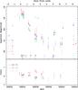 |
Fig. 1 Ground-based optical photometry of the 2014 eruption of M31N 2008-12a, all data are taken from Table 6. Epochs of optical spectra from the 2014 eruption (black lines), 2012 eruption (grey line), and the SSS behaviour (blue lines) are shown for informational purposes. Top panel: optical light curve; the dotted lines indicate a template light curve based on the V- (green) and R/r′-band (red) observations of the 2008, 2011, 2012, and 2013 eruptions, and we assume tmax = 56 933.7 (MJD) or 2014 Oct. 3.7 UT (see discussion in Sect. 4.1 and DWB14). Bottom panel: colour evolution of the 2014 eruption of M31N 2008-12a. |
3.1.1. Liverpool telescope photometry
A pre-planned broadband B, V, r′, and i′ photometry programme was initiated on the LT immediately following the LT detection of the 2014 eruption of M31N 2008-12a. Once M31N 2008-12a had faded beyond the brightness limit for LT spectroscopic observations, the LT photometric observations were supplemented with narrowband (Δλ ~ 100 Å) Hα observations.
The LT observing strategy involved taking 3 × 120 s exposures through each of the filters per epoch. The LT robotic scheduler was initially requested to repeat these observations with a minimum interval (between repeat observations) of 1 h. This minimum interval was increased to 1 day from the night beginning 2014 Oct. 11 UT. To counter the signal-to-noise losses as the nova faded, the exposure time was increased to 3 × 300 s from Oct. 5.5 UT onwards. The narrowband Hα filter was added to the program from Oct. 5.5 UT, and the observations through the broadband filters ceased from the night beginning Oct. 11 UT. LT observations following the 2014 eruption ended at Oct. 27.0 UT, and a monitoring campaign for the next eruption immediately began.
The LT data were pre-processed at the telescope and then further processed using standard routines within Starlink (Disney & Wallace 1982) and IRAF (Tody 1993). Point-spread function (PSF) fitting was performed using the Starlink photom (v1.12-2) package. Photometric calibration was achieved using 17 stars from Massey et al. (2006) within the IO:O field (see Table 2), transformations from Jester et al. (2005) were used to convert these calibration stars from BVRI to BVr′i′. In all cases, uncertainties from the photometric calibration are not the dominant source of error. The Hα data were calibrated by assuming the average Hα excess (above their r′-band emission) of the 17 calibration stars was ≃0 and by calibrating these stars’ Hα photometry relative to their r′ emission. Deviations from this assumption were ≤5 percent.
Photometry calibration stars in the field of M31N 2008-12a employed with the LT and MLO observations.
3.1.2. Mount Laguna observatory 1.0 m photometry
Photometric observations of M31N 2008-12a were carried out on 2014 October 4 UT (approximately 1.3 days after the discovery of the most recent eruption) using the MLO 1 m reflector. A series of five 120 s exposures were taken through each of the Johnson-Cousins B, V, R, I filters (see Bessell 1990), and imaged on a Loral 2048 × 2048 CCD. The data were initially processed (bias subtracted and flat-fielded) using standard routines in the IRAF software package. The individual images for a given filter were subsequently aligned to a common coordinate system and averaged forming master B, V, R, and I-band images. Calibrated B, V, R, and I magnitudes for M31N 2008-12a were then determined by comparing the instrumental magnitudes for the nova with those of five nearby secondary standard stars (#9 − #12 and #14; see Table 2) using the IRAF apphot package. The resulting magnitudes were reported in Shafter & Darnley (2014) and are given in Table 6.
3.1.3. Ondřejov observatory 0.65 m and Danish 1.54 m photometry
Photometric observations at Ondřejov started around maximum brightness of the 2014 eruption of the nova on 2014 October 3.738 UT. We used the 0.65 m telescope at the Ondřejov Observatory (operated partly by Charles University, Prague) equipped with a Moravian Instruments G2-3200 CCD camera (using a Kodak KAF-3200ME sensor and standard BVRI photometric filters) mounted at the prime focus. Observations with the Danish 1.54 m telescope at La Silla were obtained remotely from Ondřejov during two nights; when the fading nova was fainter than the R-band limit of the DFOSC instrument. The high airmass of the target observed from La Silla prevented deeper observations, despite the good observing conditions. For each epoch, a series of several 90 s exposures was taken (see Table 6 for total exposure times for each epoch). Standard reduction procedures for raw CCD images were applied (bias and dark-frame subtraction and flat field correction) using APHOT3 (Pravec et al. 1994). Reduced images within the same series were co-added to improve the signal-to-noise ratio and the gradient of the galaxy background was flattened using a spatial median filter via the SIPS4 program. Photometric measurements of the nova were then performed using aperture photometry in APHOT. Five nearby secondary standard stars (including #9 and #11 listed in Table 2) from Massey et al. (2006) were used to photometrically calibrate the magnitudes presented in Table 6.
3.1.4. iTelescope.net T11 and T24 photometry
Photometric observations of M31N 2008-12a were carried out remotely with iTelescope.net. Three 180s exposures were taken through a V-band filter using the T24 telescope (Planewave 24-inch CDK Telescope f/6.5 and a FLI PL-9000 CCD camera) at the hosting site in Sierra Remote Observatory (Auberry, CA USA) on Oct. 03.299 UT. Five 180 s exposures were taken through a V filter with same instruments on Oct. 04.214 UT. The iTelescope.net T11 telescope (Planewave 20-inch CDK telescope and FLI PL-11002M CCD camera) was also used on Oct. 04.777 UT at the New Mexico Skies hosting site near Mayhill, NM, USA. Exposure times were 5 × 180 s through a V-band filter. These images were combined and measured with the photometry function of the MIRA pro x64 software5. Ten photometric reference stars were chosen from the Fourth US Naval Observatory CCD Astrograph Catalog (UCAC4; Zacharias et al. 2013) catalog and used for photometry.
3.1.5. Kiso observatory 1.05 m photometry
Photometry of M31N 2008-12a was performed on 2014 October 3 and 6 UT using the Kiso 1.05-m Schmidt telescope, Nagano, Japan, and the KWFC instrument (Sako et al. 2012). We obtained a series of 3 × 60 s exposures in the B- and V-bands. On October 3, we also obtained a single 300 s exposure and a series of 5 × 300 s exposures in the U-band. Bias subtraction and flat-fielding were processed using standard routines within IRAF. Astrometric calibration and image co-addition were carried out using the SCAMP6 and SWarp7 software, respectively. Photometry was performed using the aperture photometry routine within SExtractor (Bertin & Arnouts 1996). With photometric calibration performed by using a number nearby 15 − 17th magnitude stars from the SDSS catalog. We used the transformations from Jester et al. (2005) to convert the magnitude system of these stars from u′g′r′ to UBV.
3.2. Optical spectroscopy
In addition to the photometric monitoring following the detection of the sixth eruption of M31N 2008-12a within seven years, spectroscopic observations were undertaken by the LT and William Herschel Telescope (WHT), co-sited on La Palma. A single, early spectrum was obtained by the WHT (hereafter, first epoch). The LT obtained daily spectra during the first three days post-discovery (second, third, and fourth epochs, respectively). The following text describes the spectroscopic observations and data reduction, with the spectra themselves presented in Fig. 3.
3.2.1. William Herschel telescope ACAM spectrum
The first epoch spectrum was obtained on 2014 Oct. 3.96 UT (exposure mid point; t − tmax = 0.26 days) at the 4.2 m William Herschel Telescope (WHT) on La Palma. We used the Auxiliary Port Camera (ACAM) in its spectroscopy mode with the V400 VPH grism and the  slit oriented at the parallactic angle. The spectrum was recorded by the 2048 × 4200 pixel EEV CCD camera under clear conditions with
  seeing and an exposure time of 300 s. A spectrum of a CuNe arc lamp was taken for wavelength calibration in the afternoon. The ACAM spectroscopic setup provided a spectral resolution of ~20 Å (full-width at half-maximum, FWHM) in the central part of the 3820 − 9495 Å useful wavelength interval.
We applied standard reduction techniques to the WHT/ ACAM spectroscopic data using IRAF tools. After bias subtraction and flat-fielding, we removed the sky background and then extracted the 1D spectrum with the optimal extraction technique of Horne (1986) as implemented in the pamela package. For the wavelength solution, we fitted a 4th-order polynomial to the pixel-wavelength arc data. The resulting wavelength scale was corrected for shifts due to instrument flexure using the O i (6300 Å) night-sky emission line. These wavelength-related procedures were carried out within the molly package8. The WHT/ACAM spectrum was later flux calibrated relative to the almost simultaneous LT SPRAT spectrum (second spectral epoch). Hence, we estimate a total flux uncertainty of ~20 percent, with an unknown (but likely small) systematic error due to the time difference between these spectra.
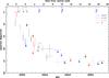 |
Fig. 2 Swift UV light curve of the 2014 eruption of M31N 2008-12a, all data are taken from Table 8. Here we assume optical maximum light occurred at 2014 Oct. 3.7 UT (see discussion in Sect. 4.1). Epochs of optical spectra from the 2014 eruption (black lines), 2012 eruption (grey line), and the SSS behaviour (blue lines) are shown for informational purposes. |
3.2.2. Liverpool telescope SPRAT spectra
Three epochs of spectroscopy of M31N 2008-12a were obtained on successive nights from 2014 Oct. 3–5 using the SPRAT spectrograph (Piascik et al. 2014) in the blue optimised mode on the LT. A slit width of  was used, yielding a spectral resolution of ~20 Å, and a velocity resolution of ~1000 km s-1 at the central wavelength of 5850 Å.
These LT spectra represent some of the first fully robotically acquired spectra taken by the newly mounted SPRAT spectrograph during its science commissioning program.
A total of 14 exposures each of duration 600 seconds, were obtained between 2014 Oct. 3.95 UT and Oct. 4.21 (mean MJD 56 934.06; t − tmax = 0.32 days; second epoch). Four exposures each of duration 1200 s were obtained between Oct. 5.13 UT and 5.23 (mean MJD 56 935.18; t − tmax = 1.44 days; third epoch). A single 1200 s exposure was obtained at 2014 Oct. 5.91 UT (t − tmax = 2.17 days; fourth epoch). All of the nights were photometric.
Following bias subtraction, flat fielding, and cosmic ray removal, data reduction was carried out using the Starlink figaro (v5.6-6; Cohen 1988) package. Sky subtraction was accomplished in the 2D images via a linear fit of the variation of the sky emission in the spatial direction (parallel to the slit). Following this, a simple extraction of the spectra was carried out. No trace of residual sky emission could be detected in the extracted spectra. The extracted spectra were then wavelength calibrated using observations of a xenon arc lamp obtained directly after each exposure, with a root mean square (rms) residual of ~1 Å. Following wavelength calibration the spectra were re-binned to a uniform wavelength scale of 6.46 Å per pixel between 4200 and 7500 Å. All of the spectra from a single night were then co-added.
Since no flux standards were observed on the nights in question, the co-added spectra were flux calibrated using observations of the spectrophotometric standard BD+28 4211 (Stone 1977) obtained on the photometric night of 2014 Sept. 4 (with the same spectrograph configuration and slit width). The spectra are therefore presented in units of Fν (mJy). Comparison of imaging observations between the calibration night and the three LT spectra show zero-point differences of <0.1 mag (i.e. <10 percent). The greatest uncertainties in the flux calibration will therefore be due to slit losses caused by seeing variations and misalignment of the object with the slit. We measure this from our repeated observations of the source on the same night to be ~15 percent. We therefore estimate a total flux uncertainty of ~20 percent.
3.3. Swift UV photometry
Immediately after the discovery of the 2014 eruption of M31N 2008-12a we requested a target of opportunity (ToO) program for the daily monitoring of the UV and X-ray emission with the Swift satellite (Gehrels et al. 2004). The X-ray data analysis and results are described in detail in HND15. Here, we analysed the Swift UV/optical telescope (UVOT; Roming et al. 2005) data and estimated the magnitude of the nova using the uvotsource tool, which performs aperture photometry. We carefully selected source and background regions to minimise any contamination by the irregular background light within the spiral arm. However, we cannot exclude the possibility that unresolved emission in our source region did cause the relatively bright, late upper limits in Fig. 2 or the apparent detection in the uvm2 filter around day 17 after maximum. All magnitudes assume the UVOT photometric system (Poole et al. 2008) and have not been corrected for extinction. The UVOT upper limits correspond to 3σ confidence. As Swift is in a low-Earth orbit, a typical observation is a series of “snapshots”, while M31N 2008-12a was bright enough to be detected in single exposures we report the snapshot photometry, otherwise we report the photometry from the combined exposures. The Swift/UVOT photometry is presented in Table 8 and the UV light curve is shown in Fig. 2.
4. Results
4.1. Maximum light and template light curves
From inspection of the 2014 optical light curve presented in Fig. 1, it appears that the optical maximum of this eruption may have been caught, or at worst marginally missed; the peak magnitudes reached in previous eruptions were V = 18.4 and R = 18.18 (see discussion in DWB14), compared to the Vmax = 18.5 ± 0.1 and Rmax = 18.2 ± 0.1 observed for this eruption (see Table 6 and Hornoch et al. 2014). As such we assume that maximum light for the 2014 eruption occurred at, or shortly before 2014 Oct. 3.7 ± 0.1 UT, and no earlier than Oct. 3.3 UT. For the analysis in this paper we assume a MJD of maximum light of tmax = 56 933.7( ± 0.1). Note, HND15 define their reference date as the time of eruption, which they assume occurred almost exactly one day before the optical peak (MJD 56 932.69 ± 0.21 d).
In DWB14, a pair of rough “template” V- and R/r′-band light curves were produced by combining the limited photometric data then available from the 2008, 2011, 2012, and 2013 eruptions. This approach made use of the supposition by Schaefer (2010) that all eruptions of a given RN are essentially identical. Given the large uncertainties in some of the data from these previous eruptions and the significantly improved temporal coverage obtained for the 2014 eruption, these original template light curves do not map well on to the 2014 data. Hence, we have updated the template light curves initially presented in DWB14 by assuming tmax of 2011 Oct. 23.49 UT, 2012 Oct. 19.72 UT, and 2013 Oct. Nov. 28.60 UT for the last three eruptions, these updated templates are shown by the dotted lines in Fig.1. The updated templates (based still only on data from previous eruptions) match the V- and R-band behaviour seen before and immediately following maximum light in the 2014 eruption very well. They only begin to deviate after ~1 day post-maximum due to the limited, and uncertain, data available at such times from earlier eruptions. However, based on data from previous eruptions, we can state that the light curve of the 2014 eruption is indeed remarkably similar to those before it.
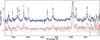 |
Fig. 3 Liverpool Telescope SPRAT and William Herschel Telescope ACAM flux calibrated spectra of the 2014 eruption of M31N 2008-12a. Blue line: (WHT) taken at 2014 Oct. 3.96 UT, t − tmax = 0.26 days (first epoch). Black line: (LT) mean time of 2014 Oct. 4.06 UT, t − tmax = 0.32 ± 0.14 days (second epoch). Red line: (LT) mean time of 2014 Oct. 5.18 UT, t − tmax = 1.44 ± 0.18 days (third epoch). Grey line: (LT) taken at 2014 Oct. 5.91 UT, t − tmax = 2.17 ± 0.01 days (fourth epoch). |
4.2. Light curve morphology
The rise from detection (≲1 mag below peak) to maximum light took just under 1 day; for a nova whose evolution post maximum is so fast, this can be considered a slow rise to peak compared to the majority of Galactic nova light curves (see, for e.g., the Galactic RN light curves presented by Schaefer 2010). The decline from maximum then proceeds rapidly, and the light curve decays approximately linearly (that is an exponential decline in the luminosity; as was also noted by TBW14 for previous eruptions) through BVRr′i′ filters until around 2 − 2.5 days post-maximum. At this stage the light curve enters a short-lived apparent “plateau” around 2 mag below peak for approximately 1 day; indeed there may also be a slight re-brightening at this stage, particularly in the V-band. Light curve plateaus have been proposed as an identifying feature of RNe (Hachisu et al. 2008), Schaefer (2010) noted that the majority of Galactic RN light curves exhibit plateaus (see also HND15), and Pagnotta & Schaefer (2014) used plateaus as one of a collection of features to identify RNe. Following this plateau, the light curve again took on an approximately linear decline (at least in the V and r′-bands), until varying seeing conditions and the unresolved M31 surface brightness rendered the eruption undetectable (last detected in the i′-band 8.148 days post-maximum). Between days 5 and 7, the BVr′i′ emission re-brightened slightly and remained approximately constant for around 1 day, before declining below the detection threshold; the i′-band emission remained at this elevated level until at least day 8. The timing of these “re-brightenings” corresponds to the emergence of the SSS (see HND15) and may be related. Despite the high cadence nature of these observations, at times significant variation was occurring that may not have been well sampled by our observations.
The narrow-band Hα photometric light curve (for which observations commenced around day 2 post-maximum, largely mirrors the r′-band light curve, as would be expected if the r′-band emission was dominated by the Hα line rather than continuum emission, as is indicated in e.g., Fig. 3. Novae routinely remain bright and detectable in narrow-band Hα imaging after they become undetectable through broad-band filters (this has driven a number of extragalactic nova surveys, see e.g., Ciardullo et al. 1987). However, in this case the Hα emission from M31N 2008-12a was undetectable ~6 days post maximum. Hα observations continued for just over a month post-eruption but no source was detected at that position (typical 5σ limiting magnitude of ~20).
Interpretation of the UV light curve is complicated by the large variation in filters (these observations typically used the Swift/UVOT “filter of the day”); however the general trend closely mirrors that of the optical light curve. Through a combination of the ground based U-band observations and the Swift/UVOT uvw2 data the time of peak in the UV light curve closely matches that in the optical. Both the UV light curve and the optical light curve show a decline of ~4 mag within the first eight days post-maximum. While the sampling of the UV data is too sparse (within a given filter) to see any evidence of a day 2 − 2.5 “plateau”, there is tentative evidence (in the U-band) for a similar “re-brightening” ~6–7 days post-maximum. M31N 2008-12a was undetectable from day 8 post maximum, however there is a Swift/UVOT uvm2 detection around day 10 (around the time of the maximum SSS emission) and a second at approximately day 16 (just around the SSS turn-off time). We speculate that this late-time UV emission could be the tail of the SSS emission (see Sect. 4.4 of HND15 for a discussion).
4.3. Spectroscopic results
The initial results from the analysis of the second epoch spectrum were reported in Darnley et al. (2014d). The spectra of the 2014 eruption (see Fig. 3) are dominated by the hydrogen Balmer emission lines (primarily Hα, but also Hβ and Hγ). The following emission lines are also clearly present in the first three epochs, He i (4471, 5017, 5876, 6678, and 7065 Å), He ii (4686 Å), N ii (5001 and 5680 Å), and N iii (4641 Å), due to the significantly decreased exposure time, these lines are not visible in the fourth epoch. No convincing evidence of Fe ii emission lines or P Cygni profiles are seen in these spectra. The flux of each emission line was calculated by fitting a simple Gaussian profile using the IRAF fitprofs command. The fitted fluxes of the Balmer and redwards He i lines are shown in Table 3; here the errors were computed by repeated fitting using different continuum determinations. The remaining emission lines show complex structures or blends, and typically low signal-to-noise. As can be seen is Table 3, there is a significant decrease in the flux from all the emission lines between the second and third epochs (t = 0.32 d and 1.44 d). If the line fluxes had remained at the levels seen in these epochs, the He i, He ii, N ii, and N iii lines could have been detected in the fourth epoch spectrum (t = 2.17 d), despite the decreased sensitivity. The first three spectra are consistent with the eruption of a nova following the initial optically thick fireball phase, and are similar to typical “He/N” spectra previously observed for M31 novae (see the extensive catalogue of Shafter et al. 2011). The morphology of the Hα emission line is shown in Fig. 5. There is a well defined central profile but with a clear double peaked structure and some evidence of higher velocity material beyond the central profile. The morphology is generally consistent with the typically “rectangular” profiles seen in He/N spectra (see e.g., Williams 2012).
Selected observed emission lines and fluxes from the three epochs of Liverpool Telescope SPRAT spectra of the 2014 eruption of M31N 2008-12a.
Continuum emission from the erupting nova is clearly detected in the first three spectra, 0.26 days, 0.32 days, and 1.44 days post-maximum, respectively. The continuum may also be marginally detected in the fourth epoch spectrum (+2.17 days). In these spectra the continuum appears essentially flat, Fig. 6 presents the deredened second epoch spectrum assuming EB − V = 0.1 and EB − V = 0.26, the lower and upper limits for the extinction towards M31N 2008-12a (see discussion in Sect. 6.2). The deredened spectra therefore show a blue continuum, as expected (see discussion in Sect. 6.1).
The spectra following the 2014 eruption are remarkably similar to those obtained after the 2012 eruption (Shafter et al. 2012, DWB14) and after the 2013 eruption (TBW14). In Fig. 4 we present a direct comparison between a spectrum obtained in 2012 from the Hobby Eberly Telescope (HET) and the second epoch spectrum from 2014. Any continuum emission was subtracted from each spectrum by fitting of a third order polynomial. These continuum-subtracted spectra were then linearly scaled. The bottom panel of Fig. 4 presents the residuals following a subtraction of these two spectra. Other than some possible structure around the Hα line, the amplitude of the residuals is consistent with the noisier 2014 spectrum.
4.4. Ejecta expansion velocity
As a proxy for the expansion velocity of the ejecta, we measured the FWHM of the Hα emission line by fitting a Gaussian profile to the central portion of the Hα line (| Δv | ≤ 4000 km s-1). In all cases a Gaussian profile provided a good fit to the emission line to below the half-maximum flux, although this profile generally did not fit well some of the extended (higher velocity) wings seen in the earlier epochs (see Fig. 5). The computed FWHM velocities for each spectral epoch are shown in Table 4, the (weighted) mean indicated FWHM expansion velocity across the four 2014 epochs is 2570 ± 120 km s-1. Such expansion velocities are consistent with the current sample of M31 He/N spectra (Shafter et al. 2011, see their Fig. 16), but they lie at the lower end of the observed distribution. The M31N 2008-12a expansion velocity is unusually low compared to other very-fast and high mass WD novae. For example, the Galactic RN U Sco exhibited Hα FWHM velocities of ~8000 km s-1 (see e.g., Anupama et al. 2013). However, such low expansion velocities are in line with predictions from the models of Prialnik & Kovetz (1995) updated in Yaron et al. (2005, see their Table 3) who show that all systems with high mass accretion rates have significantly diminished ejection velocities. Coupling a high mass accretion rate with a high mass white dwarf leads to short inter-eruption timescales.
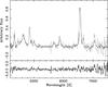 |
Fig. 4 Direct comparison between the HET spectrum of the 2012 eruption of M31N 2008-12a (t − tmax = 0.62 ± 0.1 days; black line; DWB14) and the second epoch spectrum of the 2014 eruption (LT; t − tmax = 0.26 days; grey line). Bottom panel: residuals following subtraction of the 2012 spectrum from the 2014 spectrum. |
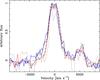 |
Fig. 5 Evolution of the Hα line profile following the 2014 eruption of M31N 2008-12a. Line colours as Fig. 3, dashed-black line indicates the Hα profile from the HET spectra following the 2012 eruption (t − tmax = 0.62 ± 0.1 days; see Fig. 4). The peak redwards of Hα is the He i (6678 Å) emission. |
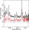 |
Fig. 6 Flux calibrated Liverpool Telescope SPRAT spectrum of the 2014 eruption of M31N 2008-12a taken 0.32 days post-maximum light (second epoch). Grey: apparent flux, red: deredened spectrum EB − V = 0.1, black: deredened spectrum EB − V = 0.26. |
Evolution of the FWHM of the Hα profile.
In the course of these FWHM determinations we have utilised a number of different approaches to determine the width of the emission lines. Most of these methods give self-consistent results, we chose the fitting of a Gaussian profile as the simplest method that utilises all the available data. Typically systematic offsets between methodologies are ~100 km s-1, and this value drives our handling of the TBW14 2013 eruption Keck spectra below.
A significant “similar implied slowing” by 510 ± 110 km s-1 is observed between the first and third 2014 epochs, with a “deceleration” by 490 ± 140 km s-1 observed between the second and third epochs. A similar implied slowing of the ejecta was noted by TBW14 following the 2013 eruption (see Table 4). For comparison, we have included the Hα FWHM velocities following the 2012 and 2013 eruptions in Table 4. Here, we have assumed maximum light times of tmax = 2012 Oct. 19.72 UT and tmax = 2013 Nov. 26.60 UT for the 2012 and 2013 eruptions, respectively. To account for any systematic uncertainties in the determination of the maximum light time we have assumed temporal uncertainties of 0.1 days and 0.2 days for the 2012 and 2013 spectra, respectively (additional uncertainty for the 2013 spectra is assumed due to lack of knowledge regarding the technicalities of these observations). Although quoted in DWB14, we have recalculated the 2012 FWHM velocity for consistency with the methodology applied here. The 2013 FWHM velocities are taken from TBW14 and we have assumed conservative uncertainties of ± 200 km s-1. The (weighted) mean FWHM velocity across the seven spectral epochs from the 2012, 2013, and 2014 eruptions is 2500 ± 70 km s-1. In Fig. 7 we show the evolution with time of the Hα profile FWHM velocity using data from the 2012, 2013, and 2014 eruptions. These data indicate a clear trend of decreasing velocity with time. These data are consistent with a linear decline of 280 ± 50 km s-1 day-1 in FWHM velocity with time (the solid black line in Fig. 7), but more detailed discussion follows in Sect. 6.3.
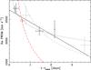 |
Fig. 7 Evolution of the FWHM of the Hα emission line following the eruption of M31N 2008-12a. Black points indicate WHT and LT spectra from the 2014 eruption, grey points are from the 2013 eruption (TBW14), and the red point is from the HET spectra in 2012 (DWB14). The solid black line shows a simple linear least-squares fit to the 2012, 2013, and 2014 data (gradient = − 280 ± 50 km s-1 day-1), the grey dashed line a power-law of index −1/3, the red dot-dashed line a power-law of index −1/2, and the black dotted line the best fit power-law with index −0.12 ± 0.05, see the text for details. |
5. Environment
An inspection of Hα images taken by the Steward 2.3 m (90-inch) Bok Telescope (BT; see Coelho et al. 2008; Franck et al. 2012, for a full description of the observation strategy) revealed extended nebulosity that appeared to surround the position of M31N 2008-12a. The Local Group Galaxies Survey (LGGS; Massey et al. 2006, 2007) narrow-band imaging data confirmed this observation, the nebulosity is visible in their Hα and [S ii] data, but is not seen in [O iii] imaging. Extended nebulosity has been seen around Galactic RNe (e.g. T Pyxidis;Shara et al. 1997; Toraskar et al. 2013) and numerous Galactic CNe (see, e.g., Slavin et al. 1995; Gill & O’Brien 1998; Downes & Duerbeck 2000); the remnants of past eruptions. In addition, nebulosity in the form of planetary nebulae, from previous evolutionary stages of the binaries, has been detected around GK Persei (Bode et al. 1987; Seaquist et al. 1989) and V458 Vulpeculae (Wesson et al. 2008), with extended shell-like H i emission being detected at even further distances from V458 Vul possibly due to mass loss during the AGB stage of the primary (Roy et al. 2012). However the apparent size of this feature around M31N 2008-12a, if directly related to the nova, would be unprecedented for any of the above phenomena.
5.1. Deep Hα imaging
To further investigate this feature, a series of 20 × 1200 s narrow-band Hα images of the region around M31N 2008-12a were taken by the IO:O camera on the LT on the night of 2014 July 30 (UT) in photometric conditions with good seeing. These images were co-aligned and a median stacked image was produced. To subtract any contribution from continuum emission from the Hα image, the 50 pre-eruption monitoring r′-band images (see Sect. 2) were aligned and median stacked, aperture photometry was then performed on 575 point sources common to both images using SExtractor (v2.19.5). A linear fit was then computed between the r′ and Hα photometry, allowing the r′ image flux to be scaled to that of the Hα image, and then subtracted9. The ~ region around the position of M31N 2008-12a in the resultant continuum subtracted Hα image is shown in Fig. 8. It is worth noting that all the Hα data referred to above would have also included any contribution from [N ii] (6548 Å and 6584 Å) emission (see also Sect. 5.2).
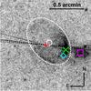 |
Fig. 8 LT Hα image (r′-band continuum subtracted and inverted) showing the |


The feature appears elliptical in nature with a semi-major axis of ~ and a semi-minor axis of ~
 (measured at the approximate midpoint of the shell-like emission; at the distance of M31 these correspond to 67 pc and 45 pc, respectively), the elliptical feature is centred at
  , δ ≃ 41°54′13″ (J2000) with a position angle on the sky of ~40°. The emission to the south-west of the ellipse is significantly brighter than that in the north-east; this emission peaks in a bright “knot” to the SW (see Sect. 5.2). The distance between the geometric centre of the nebulosity and the RN is ~4″, equivalent to a deprojected separation at the distance of M31 of ≳13 pc, this would represent a high but not completely unreasonable range for the proper motion of the RN over a large timescale.
Although larger than the majority of Galactic supernova remnants (SNRs), this feature is still somewhat smaller than the largest known Galactic SNR, GSH 138-01-94 that exhibits a radius of ~180 pc (Stil & Irwin 2001) and was discovered by virtue of its 21 cm H i emission. Assuming a mean ejecta velocity of 2500 km s-1 (see Sect. 4.3), and zero subsequent deceleration, it would take a single eruption of M31N 2008-12a between 17 000 and 27 000 yr to create a remnant of such a size.
If we also assume that the interstellar medium (ISM) density in the region of M31 around M31N 2008-12a is similar to that found in the mid-disk of the Milky Way (~0.5 M⊙ pc-3; Merrifield 1992), the ISM swept up in this volume by a single ejection event would be ~2.8 × 10⁵M⊙ (assuming a remnant geometry of a prolate spheroidal shell; see, e.g. Porter et al. 1998), which is, coincidentally, similar to that swept up by GSH 138-01-94 (although the local density there is much less as the SNR is located out of the Galactic plane). However, the kinetic energy of a nova ejecta is ~108 times less than that of a typical SN, and the momentum of the ejecta ~108 times lower, so it is clear that a single nova eruption could not create such a remnant. Although perhaps unlikely, the question remains whether multiple nova eruptions over an extended period of time could generate such a phenomenon.
While any possible association between M31N 2008-12a and the nebulosity is tantalising, it is more likely just a coincidental alignment; indeed the wider region around the RN is littered with filaments and apparent shells of gas (although none so apparently regularly shaped as that in Fig. 8). There are a number of previously identified H ii regions apparently associated with this nebulosity. The sources [AMB2011] HII 3556 (Azimlu et al. 2011, the south-western knot), [WB92a] 787 (Walterbos & Braun 1992), and [PAV78] 857 (Dodorico et al. 1980) are indicated by the green ×, white circle, and magenta box in Fig. 8, respectively. It seems clear that [WB92a] 787 is an earlier identification of the nebulosity around M31N 2008-12a, the position, size, and description (“a well defined ring”, Walterbos & Braun 1992) are consistent with our observations. The object [PAV78] 857 is identified as a SNR by (Dodorico et al. 1980), but as diffuse emission by Walterbos & Braun (1992). Finally, [JSD2012] PC 167 (the feature indicated by the blue diamond in Fig. 8) is identified as a cluster of stars (Johnson et al. 2012).
5.2. South-western “Knot” spectra
In four of our SPRAT observations of the M31N 2008-12a (see Sect. 3.2.2), the parallactic alignment of the ~ slit happened to lie across the bright knot of SW nebulosity (indicated by the green × in Fig. 8), and the resulting nebular emission could be clearly seen in the 2d spectral images. These spectra had sky position angles of 83°, 86°, 256° and 264° (see the black dashed lines in Fig. 8). For each of these spectra where the nebulosity was visible, a 3′′ wide region of the 2d image centred on the knot emission was extracted, with sky subtraction accomplished by linear fitting to a 5′′ region of sky to either side. Wavelength calibration was carried out on each individual spectrum using the corresponding arc frame, obtained directly after each exposure, which was solved for the actual rows extracted for that spectrum. The resulting spectra are therefore calibrated in wavelength to the same precision as the nova spectra (1 Å rms). All eight spectra were then resampled to a uniform pixel scale and co-added, giving a total exposure time of 6000 s. By measuring line widths of sky emission lines in the sky extraction regions, the spectral resolution of the data can be estimated as 1000 km s-1 (FWHM).
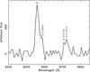 |
Fig. 9 Liverpool Telescope SPRAT spectrum of the apparent south-western “knot” in the extended emission around the position of M31N 2008-12a (solid black line; see also Fig. 8). The spectral range has been truncated to show only the region with significant emission; likely Hα, [N ii] (6584 Å), and [S ii] (6716 and 6731 Å) emission is labelled. The solid grey line indicates a simultaneous fit to the Hα and [N ii] (6584 Å) emission lines. |
Figure 9 shows the SPRAT spectrum of the SW-knot seen in Fig. 8. The spectrum is consistent with the LGGS narrow-band imaging in the sense that clear emission from Hα and [S ii] is seen, but [O iii] is not. Here the width of the spectral features is dominated by the resolution limit of SPRAT. Hence, using the morphology of a sky emission line as a template line profile, we were able to separately fit emission from the [S ii] (6716 and 6731 Å) doublet, and Hα and [N ii] (6584 Å) (see the solid grey line in Fig. 9) although any emission from [N ii] (6548 Å) was not significantly detected. The fitted central wavelength of the Hα emission from the SW-knot (6559.2 ± 0.5 Å) is consistent with that of the fitted Hα emission peak in the spectra of M31N 2008-12a (6560 ± 1 Å), and these are broadly consistent with expectation, given the blueshift of M31 (see, e.g., McConnachie 2012).
Emission from [S ii] is seen in a wide variety of astrophysical phenomena, from Herbig-Haro objects (see e.g., van den Bergh 1975) to AGN (see e.g., Busko & Steiner 1990), including, of course, SNRs. Such emission is often associated with the cooling and recombination zones behind low velocity (~100 km s-1) shocks (see e.g., Osterbrock & Dufour 1973). The [S ii]/Hα ratio is a well established criterion used for the detection of SNRs (see e.g., Mathewson & Clarke 1973; Matonick & Fesen 1997), with a ratio [S ii]/Hα ≳ 0.45 often employed for positive identification of a SNR. We determine this ratio for the SW-knot to be [S ii]/Hα = 0.35 ± 0.10 (here we have corrected for any flux contribution from [N ii], but we note that this spectrum has not been flux calibrated). At best, the [S ii]/Hα ratio is inconclusive in this case. Little, if any, evidence of [S ii] emission has yet been seen in the spectra of nova remnants (see e.g., Williams 1982, for the case of T Pyx), although Contini & Prialnik (1997) question whether any sulphur may be depleted by the formation of silicate dust grains.
5.3. Morpho-kinematical modelling of the RN spectra
Morpho-kinematical modelling of the spectra of erupting novae has been used to investigate the expansion velocity, inclination, and geometry of nova ejecta (see e.g., Ribeiro et al. 2009, 2011, 2013a,b; Shore et al. 2013a,b). Here we employed the morpho-kinematical code SHAPE (v5.0; Steffen et al. 2011) in order to ascertain whether a remnant of similar morphology to that seen in Fig. 8 could be produced by, albeit a single eruption of, an erupting nova with a Hα profile similar to that of M31N 2008-12a (as shown in Fig. 5).
To improve the spectra signal-to-noise, we co-added the four 2014 spectra with the 2012 HET spectrum of M31N 2008-12a. We introduced an ejecta density profile that varied as 1 /r3 (as modelled for V959 Monocerotis; Shore et al. 2013b), with a Hubble flow velocity distribution; essentially a free expansion. We constrained the minor to major axis ratio of the ejecta to be 2/3 (as imposed by the nebulosity; see Fig. 8), and constrained the ejecta model to a thin shell, as we observed a double peak in the eruption spectra (assuming a filling factor of unity). The inclination angle of the ejecta was also allowed to vary from 0 to 90 deg (in steps of 1 deg; where an inclination 90 deg corresponds to the orbital plane being edge-on) and the de-projected velocity varied from 2000 to 5000 km s-1 in steps of 100 km s-1. Based on the central wavelength of the Hα emission, the spectra were also corrected for a recessional velocity of ~150 km s-1.
The results of the morpho-kinematical modelling indeed suggest that a remnant geometry similar to the nebulosity seen around M31N 2008-12a can be produced by a single nova eruption exhibiting the Hα line profile seen in M31N 2008-12a. We find that such a remnant would have a bi-polar geometry, an inclination of  deg, and an expansion velocity of 1700 ± 200 km s-1. For the avoidance of doubt, it should be noted here that these are not predictions of the true nature of the M31N 2008-12a ejecta. The best-fit model spectra is shown in Fig. 10 and compared to the M31N 2008-12a Hα emission. As is evident in Fig. 10, such a simple model was unable to fit the higher velocity material (| Δv | ≥ 2000 km s-1).
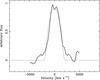 |
Fig. 10 The solid black line shows the co-added spectra from the four epochs of 2014 observations and a single epoch of 2012 observations of the erupting M31N 2008-12a, centred on the Hα emission line, (the peak redwards of Hα is the He i (6678 Å) emission). The solid grey line indicates the best-fitting model spectrum expected by a freely expanding ejecta with a bi-polar morphology, see the text for further details and discussion. |
It is important to note a number of important caveats to this work. Although we have shown that such a remnant could be produced by a nova with line profiles similar to M31N 2008-12a, our geometry solution is not likely to be unique. We imposed some constraints on the possible geometry given our limited knowledge of the system and employed a very simple model of the ejecta. A more physical model would require consideration of the ejecta interaction with the generally complex circumstellar and circumbinary environments, for example, with any red giant wind (see Sect. 6.3) as is required to model the ejecta of RS Oph (see, for e.g., Walder et al. 2008). The development of more complex models based on just these early-time spectra would likely introduce degeneracies in our results. For example, model fits to V2491 Cyg at early times replicated reasonably well the observations, however, it was not until the nebular stage that the geometry could be pinned down with some confidence (Ribeiro et al. 2011), also Della Valle et al. (2002) discuss the change in line profile due to the termination of a post-eruption wind. Finally, to produce a remnant of the scale seen in Fig. 8 it would require multiple eruptions all exhibiting similar geometries; and we would need to further consider any shaping caused by interaction with the surrounding ISM.
5.4. Follow up
The most plausible explanation for the nebulosity would be a nearby (within M31) SNR, possibly due to an association with the adjacent star cluster, which may also explain the other apparent SNR and the SW-knot; perhaps akin to some of the [S ii]-bright shell nebulae or “superbubbles” seen in the Large Magellanic Cloud (see e.g., Lasker 1977; Zhang et al. 2014). Of course, such an explanation doesn’t rule out M31N 2008-12a also being associated with this star cluster. However, none of our investigations have been able to conclusively rule out an origin related to M31N 2008-12a. Of course we must also ask ourselves, if there were not a nova near the centre of this nebula, would we still be debating its origin? However, the question of whether such a rapidly recurring nova can create a remnant as large and visible as would be required here is still an open one, and requires further observations and modelling.
6. Discussion
6.1. Spectral energy distribution
In Fig. 11 we present the evolving spectral evolution during the first three days from the peak of 2014 eruption and at quiescence (DWB14). The quiescent photometry is taken from the analysis of HST infrared, optical, and UV imaging data, as presented by DWB14. For the 2014 data, we have used optical and Swift UV absolute calibrations from Bessell (1979) and Breeveld (2010), respectively. Here we have assumed a distance to M31 of 770 ± 19 kpc (Freedman & Madore 1990), a line-of-sight external (Galactic) reddening towards M31 of EB − V = 0.1 (Stark et al. 1992), and internal (M31) reddening of EB − V ≤ 0.16 (Montalto et al. 2009). We employ the analytical Galactic mean extinction law of Cardelli et al. (1989, assuming RV = 3.1 to compute the extinction in the regime of the Swift UV filters, with no knowledge of the source spectra we simply evaluate the extinction at the central wavelength of each UV filter.
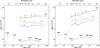 |
Fig. 11 Distance and extinction corrected SEDs showing the progenitor system of M31N 2008-12a (low luminosity black points), compared to the evolving SED of the 2014 eruption (black points, t ~ 0 days; red points, t ~ 1 days; blue points, t ~ 2 days; and grey points t ~ 3 days). Units chosen for consistency with similar plots in Schaefer (2010, see their Fig. 71) and DWB14 (see their Fig. 4). The central wavelength locations of the Johnson-Cousins, HST, and Swift filters are shown to assist the reader. Left-hand plot is the low extinction scenario, where only the line-of-sight (Galactic) extinction towards M31 is considered ( |


The optical behaviour of novae around peak has been observed to resemble black body emission (Gallagher & Ney 1976; Gehrz 2008) and has been modelled in terms of the development of a pseudo-photosphere (PP) in the optically thick ejecta (see Bath & Harkness 1989, and references therein). The PP radius rp is greatest, and effective temperature Tp at a minimum at optical peak. Thereafter, the mass loss rate from the WD surface declines, and at constant bolometric luminosity, rp shrinks while Tp rises, shifting the peak of the emission further into the UV with time past maximum light. In CNe, with relatively high ejected masses, Tp ~ 10 000 K at optical maximum placing the peak emission in the optical part of the spectrum. For a lower mass ejection rate (total mass ejected) for a given ejection velocity, the emission peak may never appear in the optical but only get as far as the UV before moving to ever higher frequencies, ultimately showing up as the SSS when the PP radius has shrunk to scales approaching that of the WD. Thus it may well be the fact that the ejected mass is far lower in an RN such as M31N 2008-12a that means these objects do not obey the MMRD (see Sect. 6.2).
From Fig. 11, one can see that at the time of optical maximum (t ~ 0), the SED does not show an obvious peak in this waveband. For the case where both the foreground Galactic and internal M31 extinctions are included (see the right-hand panel of Fig. 11), there is an indication that the peak emission is at ν ≳ 1.5 × 10¹⁵ Hz (λ ≲ 2000 Å). If emission at this time were that of a black body (as assumed for example in the simplistic models of Bath & Harkness 1989, although noting the detailed caveats given in HND15), then from the frequency dependent version of Wien’s Law, Tp ≳ 2.5 × 10⁴ K. Similarly, if we take the dereddened emission at the two highest frequency points for t ~ 0 in Table 8 (i.e., U-band and uvw2 filters) and again assume purely black body emission, then the ratio of monochromatic luminosities (Lν) at the two frequencies gives Tp ≳ 3.3 × 10⁴ K at this time.
Taking this effective temperature and Lν in the uvw2 band10, this yields an effective photospheric radius rp = 1.1 × 10¹⁰ m at optical maximum and hence a total bolometric luminosity L ~ 1032 W at this point. For LEdd = 2 × 1031 W for a WD near MCh, this implies a highly super-Eddington phase around maximum light. We note that Starrfield et al. (2008) find such a short-lived phase for a 1.35 M⊙ WD where Lmax ≳ 2 × 1032 W. We also note however that to derive a consistent solution for the absolute value of the observed dereddened monochromatic luminosity together with a self consistent bolometric luminosity, assuming purely black body emission, bolometric luminosities even higher than that derived above would be required. Black body fits to the Swift/XRT data (HND15) yield L ~ 3.3 × 1031 W (~1.8 LEdd) at later times, suggesting that any highly super-Eddington phase around the optical peak was short lived. But overall of course, great caution must be taken in over-interpreting results from simple black body assumptions when we know that the spectra at all wavelengths deviate significantly from such simplistic models (again, see discussion in HND15).
As an alternative explanation, the right panel of Fig. 11 shows spectra of optically thin free-free emission (Fν ∝ ν0) after the first epoch, with optically thick free-free emission (where e.g., Fν ∝ ν2/3 would result following Wright & Barlow 1975, for a constant mass loss rate, constant velocity, fully ionised wind) at the peak itself. Classical novae show spectra of optically thin free-free emission in their decay phase (e.g., Gallagher & Ney 1976). The brightness of free-free emission is determined mainly by the wind mass-loss rate (Wright & Barlow 1975). For a larger envelope mass at ignition, the wind mass-loss rate starts with a large value. Then the nova becomes fainter as the envelope mass decreases because the wind mass-loss rate decreases with time. Therefore, for a smaller envelope mass at ignition, the wind mass-loss rate starts with a smaller value and the nova brightness starts with a fainter maximum brightness (Hachisu & Kato 2006). The recurrence time of 1 yr requires a very massive WD (≳1.3 M⊙) and very high mass accretion rates, so the hydrogen-rich envelope mass at ignition is small. As such, this RN would be expected to have a much fainter brightness at maximum compared with CNe.
6.2. Decline time and maximum magnitude
The speed class of a nova is defined by the time taken for the light curve to decay by two or three magnitudes from peak optical luminosity, t2 and t3, respectively. Determining the speed class can be complicated by a complex light curve morphology, or by poor temporal coverage, particularly around peak luminosity. For example, the slowly evolving RN T Pyx has a long lived and complex maximum “plateau” (see e.g., Schaefer et al. 2013; Surina et al. 2014), however, the rapidly evolving RN candidate V2491 Cyg exhibits a secondary maximum in its light curve (see e.g. Darnley et al. 2011; Munari et al. 2011; Ribeiro et al. 2011, and discussions therein). The faster the decline of a given nova, the more important good determination of the peak time becomes. DWB14 estimated the decline time of the 2013 eruption to be t2(B) ≃ 5 days and t2(V) ≃ 4 days, and Hornoch et al. (2014) computed t2(R) = 2.7 ± 0.5 days based on preliminary observations of the 2014 eruption. Using the observations of the 2014 eruption, and the assumed tmax of 2014 Oct. 3.7 ± 0.1 UT, we determined the decline times shown in Table 5. Here, we assumed that the brightest observation available in each filter occurred at, or near, maximum light, and t2 and t3 times were then determined by simple linear interpolation between observations.
Decline times of the 2014 eruption of M31N 2008-12a.
The decline times for the 2014 eruption are significantly faster than those derived by DWB14 for the 2013 eruption. This is most likely due to the paucity of light curve data available at the time of that study, rather than a fundamental change in the presentation of the eruption. The value of t2(R) = 2.4 ± 0.5 days for the 2014 eruption, which is consistent with that derived using iPTF data following the 2013 eruption (t2(R) = 2.1 days; TBW14). Nova decline times are typically quoted in the V-band, partly as the early spectral evolution does not significantly affect the luminosity in this band at this time (for example, the R/r′-band t2 and t3 calculations are significantly affected by the Hα emission). With t2(V) = 1.8 ± 0.1 days and t3(V) = 3.8 ± 0.2 days, M31N 2008-12a declines more rapidly than all known Galactic RNe (surpassing U Sco with t3 = 4.3 days; see Anupama 2008), although the recently confirmed RN M31N 2006-11c (Hornoch & Shafter 2015) had a decline time of t3(R) = 3.0 ± 0.4 days during its 2015 eruption (Hornoch et al. 2015).
Based on these observations of the 2014 eruption, we can calculate the absolute magnitude at peak luminosity to be in the range −6.3 ≥ MV ≥ − 6.8, depending upon the amount of extinction internal to M31. Here we have again assumed a distance of 770 ± 19 kpc, a Galactic reddening of EB − V = 0.1, and an internal reddening of EB − V ≤ 0.16. Employing the maximum magnitude – rate of decline (MMRD) relationships derived for novae in M31 (Shafter et al. 2011) and Galactically (Downes & Duerbeck 2000), we predict the absolute magnitude of a nova as fast as M31N 2008-12a to be MV = − 9.36 ± 0.12 and MV = − 10.69 ± 0.21, respectively.
However, the MMRD relationship is known to perform poorly for RNe (see, e.g. Schaefer 2010; Hachisu & Kato 2015, their Fig. 31). Recurrence timescales as short as one year are driven by a combination of a high mass WD and high mass accretion rate, and the accreted, or ignition, mass is small (see, e.g. Yaron et al. 2005; Wolf et al. 2013; Kato et al. 2014). As such the ejected mass is too small for the PP to expand to the typical red giant size (as in CNe) hence, the effective surface temperature of the PP is always >10 000 K, the peak of the emission doesn’t move into the optical, and the optical luminosity at maximum is therefore significantly diminished (see also discussion in Sect. 6.1). Henze et al. (2014a) explore a number of different nova eruption parameter correlations for the M31 nova population; their relevance to M31N 2008-12a is discussed in HND15 (see their Sect. 4.5).
6.3. Ejecta deceleration and the nature of the system
The marked reduction with time of the width of the Hα line profile across data from the 2012, 2013, and 2014 eruptions is presented in Sect. 4.3. Such a decrease in the inferred velocity of the expanding ejecta (in the case of M31N 2008-12a, ~500 km s-1 in a ~1.2 day period) has been observed in RN systems previously. Narrowing of the emission lines following the eruptions of the Galactic RN RS Oph has been observed since at least the 1958 eruption (Dufay et al. 1964). Iijima (2009, see their Fig. 49) presents a dramatic illustration of the narrowing of the Hβ emission line following the 2006 eruption of RS Oph. In RS Oph the narrowing of the emission lines has been proposed to be caused by the deceleration of the shock driven in to the preexisting red giant wind (RGW) by the high velocity ejecta (first proposed by Pottasch 1967); the associated cooling of the shock was observed in X-rays and modelled by Bode et al. (2006). Any shocked X-ray emission from the interaction of the ejecta with surrounding material in M31N 2008-12a would not be detectable by the Swift/XRT at the distance of M31. Such a shock interaction may also give rise to optical coronal lines (e.g. [Fe xiv] (5303 Å) and [Fe x] (6374 Å)), however, in RS Oph these lines were only detected around thirty days after the eruption (Rosino 1987), and perhaps it is not surprisingly there is no evidence of any such emission in the M31N 2008-12a early-time spectra.
The RGW velocity in RS Oph is ~20 km s-1 (see Bode & Kahn 1985, and discussion therein; see also Iijima 2009, who determined a velocity of 33 km s-1), if we assume a similar red giant secondary in the M31N 2008-12a system (DWB14) and the RGW is expanding into a region fully cleared by the last eruption (a year previously), then the extent of the RGW would be ~4.2 AU. Simplistically, with an initial mean ejecta velocity of ~2700 km s-1 (see Sect. 4.3), the RGW region would begin to be cleared within ~3 days and we therefore expect a deceleration to at least this time, which covers all of our spectroscopic observations.
The HST photometry of the progenitor system of M31N 2008-12a presented by both DWB14 and TBW14 indicated the presence of a luminous accretion disk, on a par with that seen in the RS Oph system (DWB14, see their Fig. 4). The quiescent NIR photometry at the location of M31N 2008-12a was not sufficiently deep to detect the secondary star and could not rule out, for example, a secondary as luminous as that in RS Oph (DWB14). These NIR photometry were only able to exclude a secondary as luminous at that of T Coronae Borealis (the most NIR luminous quiescent RN system known; Darnley et al. 2012). With the accretion disk in the Galactic recurrent SG-Nova U Sco being at least an order of magnitude less luminous (see also the discussion regarding the distance to U Sco in Hachisu et al. 2000) than that in M31N 2008-12a, and given the results of Williams et al. (in prep.), it seems more likely that M31N 2008-12a habours a red giant secondary star.
We can now consider the observed implied deceleration in more detail. As noted above, Fig. 7 indicates that the maximum FWHM velocity at t − tmax = 0 was ~2700 km s-1 and that the derived velocity of expansion decreased systematically with time to t − tmax ≳ 3.6 days. Also shown in this figure are power-law declines in expansion velocity for strong shocks driven into the pre-existing wind of the evolved (red giant) secondary star of the system by the high velocity ejecta of the eruption. This situation is analogous to that found in RS Oph, as presented in Bode & Kahn (1985) and is described briefly here.
In the early stages of the interaction, the ejecta are still imparting energy to the shocked wind (Phase I). This is followed by a phase of adiabatic expansion (Phase II) until the shock temperature drops to the point at which the shocked gas becomes well cooled and the momentum-conserving phase of development (Phase III) is established. Plotted on Fig. 7 are functions corresponding to the expected behaviour of the observed shock velocities when the shock is traversing a wind with a 1 /r2 density distribution for Phase II (vs ∝ t− 1/3; grey dashed line) and Phase III (vs ∝ t− 1/2; red dot-dashed line).
The best fit to the data shown in Fig. 7 (black dotted line) in fact gives v ∝ t− 0.12 ± 0.05, i.e. much shallower than would be expected for either Phase II or Phase III of shocked remnant development. This type of behaviour at early times was however seen in RS Oph. Bode et al. (2006) noted that the change in slope of shock velocities derived from fits to Swift/XRT data from the 2006 eruption occurred at t ~ 6 days, in line with expectations from the Bode & Kahn (1985) model for the duration of Phase I of the eruption. Similarly, Das et al. (2006) found an abrupt steepening in velocities derived from FWHM and FWZI of infrared emission lines, again from the 2006 eruption, at t ≳ 4 days (see their Fig. 2). We thus conclude that the behaviour of the expansion velocities derived in M31N 2008-12a up to t − tmax ~ 3.6 days implies that the remnant was still in Phase I of development at this time.
From Bode & Kahn (1985), Phase I lasts for a time t ∝ Meu/Ṁve where Me and ve are the ejecta mass and initial velocity respectively, and Ṁ and u are the mass loss rate and velocity of the RGW. For simplicity, we initially assume that the latter two quantities were the same in M31N 2008-12a as in RS Oph. We can also compare the ejection velocities where ve = 5100 km s-1 in RS Oph (Ribeiro et al. 2009) and ve = 2700 km s-1 in M31N 2008-12a. Thus with Me = 2 × 10⁻⁷M⊙ (see e.g. O’Brien et al. 2006; Orlando et al. 2009) and taking the above values for the derived durations of Phase I of ≳3.6 and ~6 days in M31N 2008-12a and RS Oph respectively, this implies the total mass ejected in M31N 2008-12a is ≳3 × 10⁻⁸M⊙, which is consistent with the models presented by TBW14 and the ejected hydrogen mass as determined by HND15 (see their Sect. 4.5). There are several caveats here which include the fact that the ejection velocity derived for RS Oph by Ribeiro et al. (2009) includes the inclination to the line of sight of the ejection, but above all that the RGW parameters are assumed to be the same in the two objects, which is probably not the case.
The combination of the luminous accretion disk and the ejecta deceleration provide strong evidence in favour of M31N 2008-12a belonging to the RG-nova sub-class. However, it should also be noted that the rapidly declining CN CP Puppis (1942) also exhibited narrowing of its emissions lines (Gorbatskii 1972) and similar effects have been reported in the RNe U Sco (Munari et al. 1999) and CI Aquilae (Kiss et al. 2001). As these are novae containing a main sequence (CP Pup) or sub-giant (U Sco and CI Aql) secondary stars (see Darnley et al. 2012, and references therein) they would not be expected to contain significant circumbinary material (e.g. from stellar wind losses; however, see Williams 2013, for a recent discussion about circumbinary material around novae).
An alternative explanation for the apparent narrowing of nova ejecta emission lines is presented in Shore et al. (1996). Given the distribution of velocities within the ejecta during the onset of the eruption (see e.g., Starrfield et al. 1974), the ejected material with the highest velocity travels the furthest distance. As such, the density of this higher velocity material decreases at a faster rate than that of any lower velocity material in the ejecta, and therefore the higher the velocity of ejected material, the faster its emissivity decreases. As the ejecta expands, the apparent velocity, as derived from the spectral line profile, will decrease. Therefore, in systems with dense circumbinary material, such as the RGW around RG-novae, one would expect an combination of apparent deceleration and actual shock deceleration of the ejecta. Differentiating between the two requires more detailed observations.
The early eruption spectra of the Galactic RNe RS Oph (Iijima 2009) and V745 Scorpii (also a RG-nova; see e.g., Sekiguchi et al. 1990) both contained Fe ii emission in addition to the dominant He and N lines. The Fe ii emission lines, particularly in RS Oph, were significantly narrower (<1000 km s-1) than the Balmer, He, and N emission, and the line intensities were much lower than the He and N lines (Iijima 2009, see their Table 2). As such, the lower velocity Fe ii emission seen in RS Oph and V745 Sco has been postulated to be due to the large reservoir of circumbinary material that accumulates around those systems as a consequence of their RGWs (see Williams 2012, for a full discussion). The detection of lower velocity Fe ii emission from M31N 2008-12a could thus provide compelling evidence of a RGW. However, taking the line intensities from Iijima (2009), any such emission would be undetectable in the 2014 eruption spectra.
To unambiguously determine the secondary type in M31N 2008-12a additional observations are required, be they deeper NIR or IR imaging to detect the secondary directly, the determination of an orbital period, or sufficiently deep and high resolution eruption spectra; but at the distance of M31 the former currently seems the most feasible.
7. Summary and conclusions
In this paper we have described the discovery of the predicted 2014 eruption of M31N 2008-12a, this system’s sixth eruption in seven years. We have also presented and described the extensive optical and UV follow-up observations. Here, we summarise our findings.
-
1.
The predicted 2014 eruption of M31N 2008-12a was detected,on the rise, at 2014 Oct. 2.904 UT by a dedicated automaticpipeline put in place at the LT.
-
2.
The subsequent BVRr′i′I optical photometric monitoring campaign likely caught the point of maximum light at, or shortly before 2014 Oct. 3.7 ± 0.1 UT. The optical light curve is very similar to that of previous eruptions, notably the 2013 eruption.
-
3.
The light curve evolution was monitored with hourly cadence for first three nights post discovery, obtaining detailed multi-colour photometry that closely matched updated templates produced exclusively from previous eruptions. For periods, the photometric cadence matched that obtained for Galactic novae by the SMEI satellite (Hounsell et al. 2010, 2015), but significant variation may have been occurring on even shorter timescales.
-
4.
The optical decline time was measured as t2(V) = 1.77 ± 0.13 days and t3(V) = 3.84 ± 0.24 days, the light curve of M31N 2008-12a evolves faster than all Galactic RNe yet discovered. An early optical “plateau”, indicative of RNe, and an optical rebrightening, coinciding with the unveiling of the SSS emission, were also observed.
-
5.
Optical spectra were obtained as early as 0.26 days post-maximum light, and subsequent spectral monitoring showed remarkable similarity to the 2012 and 2013 eruptions. These spectra confirm the classification of M31N 2008-12a as an erupting nova within M31. These observations also included some of the first robotically acquired spectra from the SPRAT instrument on the LT.
-
6.
As in 2012 and 2013, the spectra are dominated by Balmer, He, and N lines, with average expansion velocity of 2570 ± 120 km s-1. A significant decrease in width of the Hα line is seen over the course of two days (510 ± 110 km s-1). The spectral evolution is remarkably similar to that seen in previous eruptions.
-
7.
Such a low ejection velocity is consistent with high mass-accretion rate, high mass WD, and short recurrence time models of TNRs.
-
8.
The low peak optical luminosity and the SED at optical maximum are consistent with a low ejected mass, TP ≳ 3.3 × 10⁴ K at this time, and the luminosity is suggested to be super-Eddington around optical peak.
-
9.
Deep Hα imaging of the quiescent system indicates the presence of an elliptical shell roughly centred at the position of the nova. While larger than even most SNRs, such an apparent alignment gives tantalising hints at an association, and deserves further study.
-
10.
Implied decreasing ejecta velocity may be caused by interaction with existing circumbinary material, most likely a red giant wind – which would cement the classification of the system as an RS Oph-like RN (RG-nova).
-
11.
Assuming a RG-nova in Phase I of remnant development, by direct analogy to the RS Oph system we can infer that the ejected mass ≳3 × 10⁻⁸M⊙, consistent with the TBW14 models.
-
12.
The monitoring campaign to detect the next eruption, predicted to occur at the end of 2015, began on 2014 Oct. 27.
Thoroughgood et al. (2001) identified the Galactic RN U Sco as the best SN Ia progenitor known, estimating that it might explode within ~700 000 yr. With its predicted very high mass WD and short inter-eruption timescale M31N 2008-12a may just have overtaken U Sco as the best single-degenerate SN Ia progenitor candidate known.
The RN M31N 2008-12a is a truly unique and remarkable system, and we strongly encourage further observation of the system and its immediate environment. We eagerly await the next eruption, which we expect to occur between October and December 2015 and for which we plan even more extensive multi-wavelength observations.
Online material
Optical photometric observations of the 2014 eruption of M31N 2008-12a.
Colour evolution of the 2014 eruption of M31N 2008-12a.
Ultraviolet photometry of the 2014 eruption of M31N 2008-12a.
A synthetic aperture photometry and astrometry software package developed by M. Velen and P. Pravec at the Ondřejov Observatory.
We assume that the spectrum of the background is similar to that of the stellar sources; which in the case of the unresolved stellar background of M31 is likely to be reasonable.
Note, here we have assumed equivalence between effective temperatures and colour temperatures.
Acknowledgments
The Liverpool Telescope is operated on the island of La Palma by Liverpool John Moores University in the Spanish Observatorio del Roque de los Muchachos of the Instituto de Astrofísica de Canarias with financial support from STFC. The William Herschel Telescope is operated on the island of La Palma by the Isaac Newton Group in the Spanish Observatorio del Roque de los Muchachos of the Instituto de Astrofísica de Canarias. Based (in part) on data collected with the Danish 1.54-m telescope at the ESO La Silla Observatory. We would like to thank the LT group at LJMU for their help, and patience, in obtaining these data from the newly commissioned SPRAT spectrograph. We are grateful to the Swift Team for making the ToO observations possible, in particular N. Gehrels, the duty scientists, as well as the science planners. The authors would like to specially thank Adam Muzzin and Mauro Stefanon for graciously donating a portion of their WHT time to this study. We thank Andrew M. Shafter (Magnolia Science Academy) for assistance with the MLO observations, Karl Misselt for taking and graciously donating the Bok data, and Phil James for advice on continuum subtraction from Hα imaging. This work used the pamela and molly software packages written by Tom Marsh. PRG acknowledges support from the MINECO under the Ramón y Cajal programme (RYC–2010–05762). K.H. was supported by the project RVO:67985815. M.H. acknowledges support from an ESA fellowship. V.A.R.M.R. acknowledges financial support from the Radboud Excellence Initiative. A.W.S. acknowledges support from NSF grant AST1009566. M.W. was supported by the Czech Science Foundation, grant P209/10/0715. This research has been supported by the Spanish Ministry of Economy and Competitiveness (MINECO) under the grants ESP2013-41268-R, AYA2011–23102, and AYA2012–38700. The comments of the referee were appreciated in identifying areas that benefited from additional discussion and clarification.
References
- Anupama, G. C. 2008 in RS Ophiuchi (2006) and the Recurrent Nova Phenomenon, eds. A. Evans, M. F. Bode, T. J. O’Brien, & M. J. Darnley (San Francisco, CA: ASP), ASP Conf. Ser., 401, 31 [Google Scholar]
- Anupama, G. C., Kamath, U. S., Ramaprakash, A. N., et al. 2013, A&A, 559, A121 [NASA ADS] [CrossRef] [EDP Sciences] [Google Scholar]
- Azimlu, M., Marciniak, R., & Barmby, P. 2011, AJ, 142, 139 [NASA ADS] [CrossRef] [Google Scholar]
- Barsukova, E., Fabrika, S., Hornoch, K., et al. 2011, ATel, 3725, 1 [NASA ADS] [Google Scholar]
- Bateson, F. M., & Hull, O. 1979, IAU Circ., 3341, 1 [NASA ADS] [Google Scholar]
- Bath, G. T., & Harkness, R. P. 1989, in Classical Novae, eds. M. F. Bode, & A. Evans (Chichester, UK: Wiley), 61 [Google Scholar]
- Bertin, E., & Arnouts, S. 1996, A&AS, 117, 393 [NASA ADS] [CrossRef] [EDP Sciences] [Google Scholar]
- Bessell, M. S. 1979, PASP, 91, 589 [NASA ADS] [CrossRef] [Google Scholar]
- Bessell, M. S. 1990, PASP, 102, 1181 [NASA ADS] [CrossRef] [Google Scholar]
- Bode, M. F. 2010, Astron. Nachr., 331, 160 [NASA ADS] [CrossRef] [Google Scholar]
- Bode, M. F., & Kahn, F. D. 1985, MNRAS, 217, 205 [NASA ADS] [CrossRef] [Google Scholar]
- Bode, M. F., & Evans, A. 2008, Classical Novae, eds. M. F. Bode, & A. Evans, 2nd edn. (Cambridge University Press), Cambridge Astrophys. Ser., 43 [Google Scholar]
- Bode, M. F., Roberts, J. A., Whittet, D. C. B., Seaquist, E. R., & Frail, D. A. 1987, Nature, 329, 519 [NASA ADS] [CrossRef] [Google Scholar]
- Bode, M. F., O’Brien, T. J., Osborne, J. P., et al. 2006, ApJ, 652, 629 [NASA ADS] [CrossRef] [Google Scholar]
- Bode, M. F., Darnley, M. J., Shafter, A. W., et al. 2009, ApJ, 705, 1056 [NASA ADS] [CrossRef] [Google Scholar]
- Breeveld, A. 2010, SWIFT-UVOT-CALDB-16-R01 [Google Scholar]
- Busko, I. C., & Steiner, J. E. 1990, MNRAS, 245, 470 [NASA ADS] [Google Scholar]
- Cao, Y., Kasliwal, M. M., Neill, J. D., et al. 2012, ApJ, 752, 133 [NASA ADS] [CrossRef] [Google Scholar]
- Cao, Y., Prince, T., Kulkarni, S. R., et al. 2014, ATel, 6532 [Google Scholar]
- Cardelli, J. A., Clayton, G. C., & Mathis, J. S. 1989, ApJ, 345, 245 [NASA ADS] [CrossRef] [Google Scholar]
- Chandrasekhar, S. 1931, ApJ, 74, 81 [NASA ADS] [CrossRef] [Google Scholar]
- Ciardullo, R., Ford, H. C., Neill, J. D., Jacoby, G. H., & Shafter, A. W. 1987, ApJ, 318, 520 [NASA ADS] [CrossRef] [Google Scholar]
- Coelho, E. A., Shafter, A. W., & Misselt, K. A. 2008, ApJ, 686, 1261 [NASA ADS] [CrossRef] [Google Scholar]
- Cohen, J. G. 1988, Instrumentation for Ground-Based Optical Astronomy (New York: Springer-Verlag), 448 [Google Scholar]
- Contini, M., & Prialnik, D. 1997, ApJ, 475, 803 [NASA ADS] [CrossRef] [Google Scholar]
- Darnley, M. J., Bode, M. F., Kerins, E., et al. 2006, MNRAS, 369, 257 [NASA ADS] [CrossRef] [Google Scholar]
- Darnley, M. J., Kerins, E., Newsam, A., et al. 2007, ApJ, 661, L45 [NASA ADS] [CrossRef] [Google Scholar]
- Darnley, M. J., Ribeiro, V. A. R. M., Bode, M. F., & Munari, U. 2011, A&A, 530, A70 [NASA ADS] [CrossRef] [EDP Sciences] [Google Scholar]
- Darnley, M. J., Ribeiro, V. A. R. M., Bode, M. F., Hounsell, R. A., & Williams, R. P. 2012, ApJ, 746, 61 [NASA ADS] [CrossRef] [Google Scholar]
- Darnley, M. J., Williams, S. C., Bode, M. F., et al. 2014a, A&A, 563, L9 (DWB14) [NASA ADS] [CrossRef] [EDP Sciences] [Google Scholar]
- Darnley, M. J., Williams, S. C., Bode, M. F., et al. 2014b, ATel, 6527 [Google Scholar]
- Darnley, M. J., Williams, S. C., Bode, M. F., et al. 2014c, ATel, 6535 [Google Scholar]
- Darnley, M. J., Steele, I. A., Smith, R. J., et al. 2014d, ATel, 6540 [Google Scholar]
- Das, R., Banerjee, D. P. K., & Ashok, N. M. 2006, ApJ, 653, L141 [NASA ADS] [CrossRef] [Google Scholar]
- Della Valle, M., Pasquini, L., Daou, D., & Williams, R. E. 2002, A&A, 390, 155 [NASA ADS] [CrossRef] [EDP Sciences] [Google Scholar]
- Disney, M. J., & Wallace, P. T. 1982, QJRAS, 23, 485 [NASA ADS] [Google Scholar]
- Dodorico, S., Dopita, M. A., & Benvenuti, P. 1980, A&AS, 40, 67 [NASA ADS] [Google Scholar]
- Downes, R. A., & Duerbeck, H. W. 2000, AJ, 120, 2007 [NASA ADS] [CrossRef] [Google Scholar]
- Dufay, J., Bloch, M., Bertaud, C., & Dufay, M. 1964, Ann. Astrophys., 27, 555 [NASA ADS] [Google Scholar]
- Evans, A., Bode, M. F., O’Brien, T. J., & Darnley, M. J. 2008, RS Ophiuchi 2006 and the Recurrent Nova Phenomenon (San Francisco, CA: ASP), ASP Conf. Ser., 401 [Google Scholar]
- Franck, J. R., Shafter, A. W., Hornoch, K., & Misselt, K. A. 2012, ApJ, 760, 13 [NASA ADS] [CrossRef] [Google Scholar]
- Freedman, W. L., & Madore, B. F. 1990, ApJ, 365, 186 [NASA ADS] [CrossRef] [Google Scholar]
- Gallagher, J. S., & Ney, E. P. 1976, ApJ, 204, L35 [NASA ADS] [CrossRef] [Google Scholar]
- Gehrels, N., Chincarini, G., Giommi, P., et al. 2004, ApJ, 611, 1005 [NASA ADS] [CrossRef] [Google Scholar]
- Gehrz, R. D. 2008, in Classical Novae, eds. M. F. Bode, & A. Evans, 2nd edn. (Cambridge: Cambridge University Press), Cambridge Astrophys. Ser., 43, 167 [Google Scholar]
- Gill, C. D., & O’Brien, T. J. 1998, MNRAS, 300, 221 [NASA ADS] [CrossRef] [Google Scholar]
- Gorbatskii, V. G. 1972, Soviet Ast., 16, 32 [NASA ADS] [Google Scholar]
- Gutierrez, J., Garcia-Berro, E., Iben, I., Jr., et al. 1996, ApJ, 459, 701 [NASA ADS] [CrossRef] [Google Scholar]
- Hachisu, I., & Kato, M. 2006, ApJS, 167, 59 [NASA ADS] [CrossRef] [Google Scholar]
- Hachisu, I., & Kato, M. 2015, ApJ, 798, 76 [NASA ADS] [CrossRef] [Google Scholar]
- Hachisu, I., Kato, M., Nomoto, K., & Umeda, H. 1999a, ApJ, 519, 314 [NASA ADS] [CrossRef] [Google Scholar]
- Hachisu, I., Kato, M., & Nomoto, K. 1999b, ApJ, 522, 487 [NASA ADS] [CrossRef] [Google Scholar]
- Hachisu, I., Kato, M., Kato, T., Matsumoto, K., & Nomoto, K. 2000, ApJ, 534, L189 [NASA ADS] [CrossRef] [PubMed] [Google Scholar]
- Hachisu, I., Kato, M., Kiyota, S., et al. 2008, in RS Ophiuchi (2006) and the Recurrent Nova Phenomenon, eds. A. Evans, M. F. Bode, T. J. O’Brien, & M. J. Darnley (San Francisco, CA: ASP), ASP Conf. Ser., 401, 206 [Google Scholar]
- Henze, M., Pietsch, W., Haberl, F., et al. 2014a, A&A, 563, A2 [NASA ADS] [CrossRef] [EDP Sciences] [Google Scholar]
- Henze, M., Ness, J.-U., Darnley, M. J., et al. 2014b, A&A, 563, L8 (HND14) [NASA ADS] [CrossRef] [EDP Sciences] [Google Scholar]
- Henze, M., Ness, J.-U., Darnley, M. J., et al. 2015, A&A, 580, A46 [NASA ADS] [CrossRef] [EDP Sciences] [Google Scholar]
- Horne, K. 1986, PASP, 98, 609 [NASA ADS] [CrossRef] [EDP Sciences] [Google Scholar]
- Hornoch, K., & Shafter, A. W. 2015, ATel, 7116 [Google Scholar]
- Hornoch, K., Kucakova, H., & Wolf, M. 2014, ATel, 6546 [Google Scholar]
- Hornoch, K., Kucakova, H., Vrastil, J., et al. 2015, ATel, 7142 [Google Scholar]
- Hounsell, R., Bode, M. F., Hick, P. P., et al. 2010, ApJ, 724, 480 [NASA ADS] [CrossRef] [EDP Sciences] [Google Scholar]
- Hounsell, R., Darnley, M. J., Bode, M. F., et al. 2015, ApJ, submitted [Google Scholar]
- Iijima, T. 2009, A&A, 505, 287 [NASA ADS] [CrossRef] [EDP Sciences] [Google Scholar]
- Jester, S., Schneider, D. P., Richards, G. T., et al. 2005, AJ, 130, 873 [NASA ADS] [CrossRef] [Google Scholar]
- Johnson, L. C., Seth, A. C., Dalcanton, J. J., et al. 2012, ApJ, 752, 95 [NASA ADS] [CrossRef] [Google Scholar]
- Kato, M., Saio, H., Hachisu, I., & Nomoto, K. 2014, ApJ, 793, 136 [NASA ADS] [CrossRef] [Google Scholar]
- Kerins, E., Darnley, M. J., Duke, J. P., et al. 2010, MNRAS, 409, 247 [NASA ADS] [CrossRef] [Google Scholar]
- Kiss, L. L., Thomson, J. R., Ogloza, W., Furész, G., & Sziládi, K. 2001, A&A, 366, 858 [NASA ADS] [CrossRef] [EDP Sciences] [Google Scholar]
- Korotkiy, S., & Elenin, L. 2010, CBAT, http://www.cbat.eps.harvard.edu/unconf/followups/J00452885+4154094.html [Google Scholar]
- Kraft, R. P. 1964, ApJ, 139, 457 [NASA ADS] [CrossRef] [Google Scholar]
- Lasker, B. M. 1977, ApJ, 212, 390 [NASA ADS] [CrossRef] [Google Scholar]
- Massey, P., Olsen, K. A. G., Hodge, P. W., et al. 2006, AJ, 131, 2478 [NASA ADS] [CrossRef] [Google Scholar]
- Massey, P., McNeill, R. T., Olsen, K. A. G., et al. 2007, AJ, 134, 2474 [NASA ADS] [CrossRef] [Google Scholar]
- Mathewson, D. S., & Clarke, J. N. 1973, ApJ, 180, 725 [NASA ADS] [CrossRef] [Google Scholar]
- Matonick, D. M., & Fesen, R. A. 1997, ApJS, 112, 49 [NASA ADS] [CrossRef] [Google Scholar]
- McConnachie, A. W. 2012, AJ, 144, 4 [NASA ADS] [CrossRef] [Google Scholar]
- Merrifield, M. R. 1992, AJ, 103, 1552 [NASA ADS] [CrossRef] [Google Scholar]
- Montalto, M., Seitz, S., Riffeser, A., et al. 2009, A&A, 507, 283 [NASA ADS] [CrossRef] [EDP Sciences] [Google Scholar]
- Munari, U., Zwitter, T., Tomov, T., et al. 1999, A&A, 347, L39 [NASA ADS] [Google Scholar]
- Munari, U., Siviero, A., Dallaporta, S., et al. 2011, New A, 16, 209 [Google Scholar]
- Nishiyama, K., & Kabashima, F. 2008, CBAT, http://www.cbat.eps.harvard.edu/iau/CBAT_M31.html#2008-12a [Google Scholar]
- Nishiyama, K., & Kabashima, F. 2012, CBAT, http://www.cbat.eps.harvard.edu/unconf/followups/J00452884+4154095.html [Google Scholar]
- O’Brien, T. J., Bode, M. F., Porcas, R. W., et al. 2006, Nature, 442, 279 [NASA ADS] [CrossRef] [PubMed] [Google Scholar]
- Orlando, S., Drake, J. J., & Laming, J. M. 2009, A&A, 493, 1049 [NASA ADS] [CrossRef] [EDP Sciences] [Google Scholar]
- Osterbrock, D. E., & Dufour, R. J. 1973, ApJ, 185, 441 [NASA ADS] [CrossRef] [Google Scholar]
- Overbeek, D., McNaught, R. H., Whitelock, P., Cragg, T., & Verdenet, M. 1987, IAU Circ., 4395, 1 [NASA ADS] [Google Scholar]
- Pagnotta, A., & Schaefer, B. E. 2014, ApJ, 788, 164 [NASA ADS] [CrossRef] [Google Scholar]
- Pagnotta, A., Schaefer, B. E., Xiao, L., Collazzi, A. C., & Kroll, P. 2009, AJ, 138, 1230 [NASA ADS] [CrossRef] [Google Scholar]
- Piascik, A. S., Steele, I. A., Bates, S. D., et al. 2014, Proc. SPIE, 9147, 91478 [Google Scholar]
- Pietsch, W., Haberl, F., Sala, G., et al. 2007, A&A, 465, 375 [NASA ADS] [CrossRef] [EDP Sciences] [Google Scholar]
- Pietsch, W., Henze, M., Haberl, F., et al. 2011, A&A, 531, A22 [NASA ADS] [CrossRef] [EDP Sciences] [Google Scholar]
- Poole, T. S., Breeveld, A. A., Page, M. J., et al. 2008, MNRAS, 383, 627 [NASA ADS] [CrossRef] [Google Scholar]
- Porter, J. M., O’Brien, T. J., & Bode, M. F. 1998, MNRAS, 296, 943 [NASA ADS] [CrossRef] [Google Scholar]
- Pottasch, S. R. 1967, Bull. Astron. Inst. Netherlands, 19, 227 [NASA ADS] [Google Scholar]
- Pravec, P., Hudec, R., Soldán, J., Sommer, M., & Schenkl, K. H. 1994, Exp. Astron., 5, 375 [NASA ADS] [CrossRef] [Google Scholar]
- Prialnik, D., & Kovetz, A. 1995, ApJ, 445, 789 [NASA ADS] [CrossRef] [Google Scholar]
- Ribeiro, V. A. R. M., Bode, M. F., Darnley, M. J., et al. 2009, ApJ, 703, 1955 [NASA ADS] [CrossRef] [Google Scholar]
- Ribeiro, V. A. R. M., Darnley, M. J., Bode, M. F., et al. 2011, MNRAS, 412, 1701 [NASA ADS] [CrossRef] [Google Scholar]
- Ribeiro, V. A. R. M., Munari, U., & Valisa, P. 2013a, ApJ, 768, 49 [NASA ADS] [CrossRef] [Google Scholar]
- Ribeiro, V. A. R. M., Bode, M. F., Darnley, M. J., et al. 2013b, MNRAS, 433, 1991 [NASA ADS] [CrossRef] [Google Scholar]
- Roming, P. W. A., Kennedy, T. E., Mason, K. O., et al. 2005, Space Sci. Rev., 120, 95 [NASA ADS] [CrossRef] [Google Scholar]
- Rosino, L. 1987, in RS Ophiuchi 1985 and the Recurrent Nova Phenomenon, ed. M. F. Bode (Utrecht: VNU Science Press), 1 [Google Scholar]
- Roy, N., Kantharia, N. G., Eyres, S. P. S., et al. 2012, MNRAS, 427, L55 [NASA ADS] [CrossRef] [Google Scholar]
- Sako, S., Aoki, T., Doi, M., et al. 2012, Proc. SPIE, 8446, 84466 [CrossRef] [Google Scholar]
- Schaefer, B. E. 2010, ApJS, 187, 275 [NASA ADS] [CrossRef] [Google Scholar]
- Schaefer, B. E., Landolt, A. U., Linnolt, M., et al. 2013, ApJ, 773, 55 [NASA ADS] [CrossRef] [Google Scholar]
- Seaquist, E. R., Bode, M. F., Frail, D. A., et al. 1989, ApJ, 344, 805 [NASA ADS] [CrossRef] [Google Scholar]
- Sekiguchi, K., Whitelock, P. A., Feast, M. W., et al. 1990, MNRAS, 246, 78 [NASA ADS] [Google Scholar]
- Shafter, A. W. 1997, ApJ, 487, 226 [NASA ADS] [CrossRef] [Google Scholar]
- Shafter, A. W., & Darnley, M. J. 2014, ATel, 6543 [Google Scholar]
- Shafter, A. W., Rau, A., Quimby, R. M., et al. 2009, ApJ, 690, 1148 [NASA ADS] [CrossRef] [Google Scholar]
- Shafter, A. W., Darnley, M. J., Hornoch, K., et al. 2011, ApJ, 734, 12 [Google Scholar]
- Shafter, A. W., Hornoch, K., Ciardullo, J. V. R., Darnley, M. J., & Bode, M. F. 2012, ATel, 4503 [Google Scholar]
- Shafter, A. W., Henze, M., Rector, T. A., et al. 2015, ApJS, 216, 34 [NASA ADS] [CrossRef] [Google Scholar]
- Shara, M. M., Zurek, D. R., Williams, R. E., et al. 1997, AJ, 114, 258 [NASA ADS] [CrossRef] [Google Scholar]
- Shore, S. N., Kenyon, S. J., Starrfield, S., & Sonneborn, G. 1996, ApJ, 456, 717 [NASA ADS] [CrossRef] [Google Scholar]
- Shore, S. N., Schwarz, G. J., De Gennaro Aquino, I., et al. 2013a, A&A, 549, A140 [NASA ADS] [CrossRef] [EDP Sciences] [Google Scholar]
- Shore, S. N., De Gennaro Aquino, I., Schwarz, G. J., et al. 2013b, A&A, 553, A123 [NASA ADS] [CrossRef] [EDP Sciences] [Google Scholar]
- Slavin, A. J., O’Brien, T. J., & Dunlop, J. S. 1995, MNRAS, 276, 353 [NASA ADS] [CrossRef] [Google Scholar]
- Stark, A. A., Gammie, C. F., Wilson, R. W., et al. 1992, ApJS, 79, 77 [NASA ADS] [CrossRef] [Google Scholar]
- Starrfield, S., Sparks, W. M., & Truran, J. W. 1974, ApJS, 28, 247 [NASA ADS] [CrossRef] [Google Scholar]
- Starrfield, S., Sparks, W. M., & Truran, J. W. 1976, in Structure and Evolution of Close Binary Systems, eds. P. Eggleton, S. Mitton, & J. Whelan (Dordrecht: D. Reidel Publishing Co.), IAU Symp., 73, 155 [Google Scholar]
- Starrfield, S., Iliadis, C., & Hix, W. R. 2008, in Classical Novae, eds. M. F. Bode, & A. Evans, 2nd edn. (Cambridge: Cambridge University Press), Cambridge Astrophys. Ser., 43, 77 [Google Scholar]
- Steele, I. A., Smith, R. J., Rees, P. C., et al. 2004, Proc. SPIE, 5489, 679 [NASA ADS] [CrossRef] [Google Scholar]
- Steffen, W., Koning, N., Wenger, S., Morisset, C., & Magnor, M. 2011, IEEE Transactions on Visualization and Computer Graphics, 17, 454 [Google Scholar]
- Stil, J. M., & Irwin, J. A. 2001, ApJ, 563, 816 [NASA ADS] [CrossRef] [Google Scholar]
- Stone, R. P. S. 1977, ApJ, 218, 767 [NASA ADS] [CrossRef] [Google Scholar]
- Surina, F., Hounsell, R. A., Bode, M. F., et al. 2014, AJ, 147, 107 [NASA ADS] [CrossRef] [Google Scholar]
- Tang, S., Cao, Y., & Kasliwal, M. M. 2013, ATel, 5607 [Google Scholar]
- Tang, S., Bildsten, L., Wolf, W. M., et al. 2014, ApJ, 786, 61 (TBW14) [NASA ADS] [CrossRef] [Google Scholar]
- Thoroughgood, T. D., Dhillon, V. S., Littlefair, S. P., Marsh, T. R., & Smith, D. A. 2001, MNRAS, 327, 1323 [NASA ADS] [CrossRef] [Google Scholar]
- Tody, D. 1993, Astronomical Data Analysis Software and Systems II, 52, 173 [NASA ADS] [Google Scholar]
- Toraskar, J., Mac Low, M.-M., Shara, M. M., & Zurek, D. R. 2013, ApJ, 768, 48 [NASA ADS] [CrossRef] [Google Scholar]
- van den Bergh, S. 1975, PASP, 87, 405 [NASA ADS] [CrossRef] [Google Scholar]
- Walder, R., Folini, D., & Shore, S. N. 2008, A&A, 484, L9 [NASA ADS] [CrossRef] [EDP Sciences] [Google Scholar]
- Walterbos, R. A. M., & Braun, R. 1992, A&AS, 92, 625 [NASA ADS] [Google Scholar]
- Wesson, R., Barlow, M. J., Corradi, R. L. M., et al. 2008, ApJ, 688, L21 [NASA ADS] [CrossRef] [Google Scholar]
- Williams, R. 2012, AJ, 144, 98 [NASA ADS] [CrossRef] [Google Scholar]
- Williams, R. 2013, AJ, 146, 55 [NASA ADS] [CrossRef] [Google Scholar]
- Williams, R. E. 1982, ApJ, 261, 170 [NASA ADS] [CrossRef] [Google Scholar]
- Williams, B. F., Garcia, M. R., Kong, A. K. H., et al. 2004, ApJ, 609, 735 [NASA ADS] [CrossRef] [Google Scholar]
- Williams, S. C., Darnley, M. J., Bode, M. F., & Shafter, A. W. 2013, ATel, 5611 [Google Scholar]
- Williams, S. C., Darnley, M. J., Bode, M. F., Keen, A., & Shafter, A. W. 2014, ApJS, 213, 10 [NASA ADS] [CrossRef] [Google Scholar]
- Wolf, W. M., Bildsten, L., Brooks, J., & Paxton, B. 2013, ApJ, 777, 136 [NASA ADS] [CrossRef] [Google Scholar]
- Woudt, P. A., & Ribeiro, V. A. R. M. 2014, Stellar Novae: Past and Future Decades (San Francisco, CA: ASP) ASP Conf. Ser., 490 [Google Scholar]
- Whelan, J., & Iben, I., Jr. 1973, ApJ, 186, 1007 [NASA ADS] [CrossRef] [Google Scholar]
- White, N. E., Giommi, P., Heise, J., Angelini, L., & Fantasia, S. 1995, ApJ, 445, L125 [NASA ADS] [CrossRef] [Google Scholar]
- Wright, A. E., & Barlow, M. J. 1975, MNRAS, 170, 41 [NASA ADS] [CrossRef] [Google Scholar]
- Yaron, O., Prialnik, D., Shara, M. M., & Kovetz, A. 2005, ApJ, 623, 398 [NASA ADS] [CrossRef] [Google Scholar]
- Zacharias, N., Finch, C. T., Girard, T. M., et al. 2013, AJ, 145, 44 [NASA ADS] [CrossRef] [EDP Sciences] [Google Scholar]
- Zhang, N.-X., Chu, Y.-H., Williams, R. M., et al. 2014, ApJ, 792, 58 [NASA ADS] [CrossRef] [Google Scholar]
All Tables
Photometry calibration stars in the field of M31N 2008-12a employed with the LT and MLO observations.
Selected observed emission lines and fluxes from the three epochs of Liverpool Telescope SPRAT spectra of the 2014 eruption of M31N 2008-12a.
All Figures
|
Fig. 1 Ground-based optical photometry of the 2014 eruption of M31N 2008-12a, all data are taken from Table 6. Epochs of optical spectra from the 2014 eruption (black lines), 2012 eruption (grey line), and the SSS behaviour (blue lines) are shown for informational purposes. Top panel: optical light curve; the dotted lines indicate a template light curve based on the V- (green) and R/r′-band (red) observations of the 2008, 2011, 2012, and 2013 eruptions, and we assume tmax = 56 933.7 (MJD) or 2014 Oct. 3.7 UT (see discussion in Sect. 4.1 and DWB14). Bottom panel: colour evolution of the 2014 eruption of M31N 2008-12a. |
| In the text | |
|
Fig. 2 Swift UV light curve of the 2014 eruption of M31N 2008-12a, all data are taken from Table 8. Here we assume optical maximum light occurred at 2014 Oct. 3.7 UT (see discussion in Sect. 4.1). Epochs of optical spectra from the 2014 eruption (black lines), 2012 eruption (grey line), and the SSS behaviour (blue lines) are shown for informational purposes. |
| In the text | |
|
Fig. 3 Liverpool Telescope SPRAT and William Herschel Telescope ACAM flux calibrated spectra of the 2014 eruption of M31N 2008-12a. Blue line: (WHT) taken at 2014 Oct. 3.96 UT, t − tmax = 0.26 days (first epoch). Black line: (LT) mean time of 2014 Oct. 4.06 UT, t − tmax = 0.32 ± 0.14 days (second epoch). Red line: (LT) mean time of 2014 Oct. 5.18 UT, t − tmax = 1.44 ± 0.18 days (third epoch). Grey line: (LT) taken at 2014 Oct. 5.91 UT, t − tmax = 2.17 ± 0.01 days (fourth epoch). |
| In the text | |
|
Fig. 4 Direct comparison between the HET spectrum of the 2012 eruption of M31N 2008-12a (t − tmax = 0.62 ± 0.1 days; black line; DWB14) and the second epoch spectrum of the 2014 eruption (LT; t − tmax = 0.26 days; grey line). Bottom panel: residuals following subtraction of the 2012 spectrum from the 2014 spectrum. |
| In the text | |
|
Fig. 5 Evolution of the Hα line profile following the 2014 eruption of M31N 2008-12a. Line colours as Fig. 3, dashed-black line indicates the Hα profile from the HET spectra following the 2012 eruption (t − tmax = 0.62 ± 0.1 days; see Fig. 4). The peak redwards of Hα is the He i (6678 Å) emission. |
| In the text | |
|
Fig. 6 Flux calibrated Liverpool Telescope SPRAT spectrum of the 2014 eruption of M31N 2008-12a taken 0.32 days post-maximum light (second epoch). Grey: apparent flux, red: deredened spectrum EB − V = 0.1, black: deredened spectrum EB − V = 0.26. |
| In the text | |
|
Fig. 7 Evolution of the FWHM of the Hα emission line following the eruption of M31N 2008-12a. Black points indicate WHT and LT spectra from the 2014 eruption, grey points are from the 2013 eruption (TBW14), and the red point is from the HET spectra in 2012 (DWB14). The solid black line shows a simple linear least-squares fit to the 2012, 2013, and 2014 data (gradient = − 280 ± 50 km s-1 day-1), the grey dashed line a power-law of index −1/3, the red dot-dashed line a power-law of index −1/2, and the black dotted line the best fit power-law with index −0.12 ± 0.05, see the text for details. |
| In the text | |
|
Fig. 8 LT Hα image (r′-band continuum subtracted and inverted) showing the |
| In the text | |
|
Fig. 9 Liverpool Telescope SPRAT spectrum of the apparent south-western “knot” in the extended emission around the position of M31N 2008-12a (solid black line; see also Fig. 8). The spectral range has been truncated to show only the region with significant emission; likely Hα, [N ii] (6584 Å), and [S ii] (6716 and 6731 Å) emission is labelled. The solid grey line indicates a simultaneous fit to the Hα and [N ii] (6584 Å) emission lines. |
| In the text | |
|
Fig. 10 The solid black line shows the co-added spectra from the four epochs of 2014 observations and a single epoch of 2012 observations of the erupting M31N 2008-12a, centred on the Hα emission line, (the peak redwards of Hα is the He i (6678 Å) emission). The solid grey line indicates the best-fitting model spectrum expected by a freely expanding ejecta with a bi-polar morphology, see the text for further details and discussion. |
| In the text | |
|
Fig. 11 Distance and extinction corrected SEDs showing the progenitor system of M31N 2008-12a (low luminosity black points), compared to the evolving SED of the 2014 eruption (black points, t ~ 0 days; red points, t ~ 1 days; blue points, t ~ 2 days; and grey points t ~ 3 days). Units chosen for consistency with similar plots in Schaefer (2010, see their Fig. 71) and DWB14 (see their Fig. 4). The central wavelength locations of the Johnson-Cousins, HST, and Swift filters are shown to assist the reader. Left-hand plot is the low extinction scenario, where only the line-of-sight (Galactic) extinction towards M31 is considered ( |
| In the text | |
Current usage metrics show cumulative count of Article Views (full-text article views including HTML views, PDF and ePub downloads, according to the available data) and Abstracts Views on Vision4Press platform.
Data correspond to usage on the plateform after 2015. The current usage metrics is available 48-96 hours after online publication and is updated daily on week days.
Initial download of the metrics may take a while.