| Issue |
A&A
Volume 580, August 2015
|
|
|---|---|---|
| Article Number | A66 | |
| Number of page(s) | 21 | |
| Section | Stellar structure and evolution | |
| DOI | https://doi.org/10.1051/0004-6361/201525756 | |
| Published online | 04 August 2015 | |
Stellar rotation, binarity, and lithium in the open cluster IC 4756⋆,⋆⋆
1 Leibniz-Institute for Astrophysics Potsdam (AIP), An der Sternwarte 16, 14482 Potsdam, Germany
e-mail: This email address is being protected from spambots. You need JavaScript enabled to view it.
; This email address is being protected from spambots. You need JavaScript enabled to view it.
; This email address is being protected from spambots. You need JavaScript enabled to view it.
; This email address is being protected from spambots. You need JavaScript enabled to view it.
; This email address is being protected from spambots. You need JavaScript enabled to view it.
; This email address is being protected from spambots. You need JavaScript enabled to view it.
2 Space Science Institute, 4750 Walnut Street #205, Boulder, CO 80301, USA
Received: 27 January 2015
Accepted: 2 March 2015
Abstract
Context. An important aspect in the evolutionary scenario of cool stars is their rotation and the rotationally induced magnetic activity and interior mixing. Stars in open clusters are particularly useful tracers for these aspects because of their known ages.
Aims. We aim to characterize the open cluster IC 4756 and measure stellar rotation periods and surface differential rotation for a sample of its member stars.
Methods. Thirty-seven cluster stars were observed continuously with the CoRoT satellite for 78 days in 2010. Follow-up high-resolution spectroscopy of the CoRoT targets and deep Strömgren uvbyβ and Hα photometry of the entire cluster were obtained with our robotic STELLA facility and its echelle spectrograph and wide-field imager, respectively.
Results. We determined high-precision photometric periods for 27 of the 37 CoRoT targets and found values between 0.155 and 11.4 days. Twenty of these are rotation periods. Twelve targets are spectroscopic binaries of which 11 were previously unknown; orbits are given for six of them. Six targets were found that show evidence of differential rotation with ΔΩ/Ω in the range 0.04−0.15. Five stars are non-radially pulsating stars with fundamental periods of below 1 d, two stars are semi-contact binaries, and one target is a micro-flaring star that also shows rotational modulation. Nine stars in total were not considered members because of much redder color(s) and deviant radial velocities with respect to the cluster mean. Hα photometry indicates that the cluster ensemble does not contain magnetically over-active stars. The cluster average metallicity is –0.08 ± 0.06 (rms) and its logarithmic lithium abundance for 12 G-dwarf stars is 2.39 ± 0.17 (rms).
Conclusions. The cluster is 890 ± 70 Myrs old with an average turn-off mass of 1.8 M⊙ and a solar or slightly subsolar metallicity. The distance modulus is 8m.02 and the average reddening E(b - y) = 0m.16.. The cluster is masked by a very inhomogeneous foreground and background dust distribution and our survey covered 38% of the cluster. The average lithium abundance and the rotation periods in the range 1.7 to 11.4 d are consistent with the cluster age.
Key words: stars: rotation / stars: activity / stars: late-type / starspots / open clusters and associations: individual: IC 4756 / stars: oscillations
The CoRoT space mission has been developed and is operated by CNES, with the contribution of Austria, Belgium, Brazil, ESA (RSSD and Science Programme), Germany and Spain. Partly based on data obtained with the STELLA robotic observatory in Tenerife, an AIP facility jointly operated by AIP and IAC.
Appendices are available in electronic form at http://www.aanda.org
© ESO, 2015
1. Introduction
Stellar surface rotation and differential rotation are crucial to our understanding of magnetic activity of late-type stars. The rotation periods of stars in open clusters with well-determined ages will not only confirm the gyro-ages put forward in previous years by Barnes (2007; 2010), but will also help to quantitatively establish the angular-momentum transport mechanism as a function of stellar evolution (Barnes & Kim 2010; Gallet & Bouvier 2013; Meibom et al. 2013; 2015). The magnitude and sign of the surface differential rotation pattern can even specify the role of the stellar magnetic field because differential rotation constrains the large-scale magnetic surface configurations, and will tell us about the underlying dynamo process (e.g., Küker et al. 2011; Käpylä et al. 2013; Hathaway et al. 2013; Rüdiger et al. 2014).
Rotation can be recovered from the spot modulation in time-series photometry, either from the ground via decade-long coverage with small robotic telescopes (e.g., Henry 1999; Oláh et al. 2003; Strassmeier 2009) or from space with comparatively short runs but basically perfect sampling (e.g., for CoRoT-2a; Fröhlich et al. 2009). For space-based observations, we are confident that even if a spot configuration is less favorable than CoRoT-2a, a unique interpretation is possible from the clean window function and the high photometric precision (e.g., Reinhold et al. 2013). Furthermore, inversion of a time series using a spot-modeling approach also allows the extraction of spot longitudes and fractional spot coverage (e.g., Strassmeier & Bopp 1992; Lanza et al. 2009; Savanov & Dmitrienko 2012; Roettenbacher et al. 2013).
An essential role for rotational studies of open clusters is to relate stellar properties to the general cluster properties. Among these properties are a cluster’s turn-off age and average metallicity and also the lithium abundance and dispersion of its G dwarfs in order to relate eventual models to the Sun as a star. While space-based photometry is clearly superior for periodicities of various sorts, ground-based multi-band photometry and follow-up spectroscopy are essential in determining membership, abundances, and binarity (see, e.g., Meibom et al. 2011; Milliman et al. 2014). We have therefore used the CoRoT satellite (Baglin et al. 2006) in its sixth long run to observe selected and bona fide member stars of the open cluster IC 4756 that happened to be within the exoplanet field of view of the satellite. From the ground, we employed our robotic STELLA facility with its wide-field imager and echelle spectrograph. With an age of ≈800 Myr (Salaris et al. 2004) IC 4756 is nearly coeval with the Hyades where spot activity is weak but still present. The expected range of rotation periods for single stars is 2−20 days while the suggested turn-off mass is around 1.8−1.9 M⊙ (Mermillod & Mayor 1990). Precise periods for IC 4756 could be important for our understanding of rotational evolution of low-mass stars because all current rotational evolutionary models for above age are constrained (and restricted) by the statistics driven by the Hyades cluster (see Irwin & Bouvier 2009).
In the current paper, we present CoRoT time-series photometry for 37 of our initial 38 targets in the field of IC 4756 – one of the initial 38 targets was not observed in the end – and determine precise rotational periods for 20 of them. Deep Strömgren uvbyβ and Hα photometry was obtained with our robotic STELLA facility to obtain a color−magnitude diagram (CMD) and also to determine effective temperatures, gravities, metallicities, and an Hα-based activity measure for the detectable cluster members. STELLA has also been used to obtain high-resolution spectra to determine radial velocities (RVs), lithium abundances, and other astrophysical properties. One target, HSS 348, has been observed and is being analyzed in more detail in a separate paper.
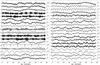 |
Fig. 1 CoRoT light curves for the target stars from Table 1. The running number on the left side of the plots identifies each star. The numbers on the right side of each plot indicate the scale (varying from star to star) in millimag. Star #2 is missing because CoRoT photometry could not be obtained for it. |
2. Observations and data reductions
2.1. CoRoT photometry
CoRoT observed IC 4756 from 2010 July 8 to September 24 (long run LRc06; 78 days). One of the two CCDs for the exoplanet field was used, and stars between B ≈ 10−14 mag were downloaded. Almost the entire cluster was observable by CoRoT. The cluster’s angular diameter has been estimated by Herzog et al. (1975) to be around 90′.
Our full (38-star) CoRoT IC4756 sample is summarized in Table 1 and the photometry is shown in Fig. 1. The principal identifier used in this paper is running number in the first column in Table 1. The following columns list the Herzog-Sanders-Seggewiss (HSS) number, the USNO-B1.0 number, a cluster membership flag, followed by the NOMAD coordinates (Zacharias et al. 2005). V magnitudes are taken from NOMAD while the B−V values are from Herzog et al. (1975). The next three columns list our RVs from STELLA/SES, with an rms value listed when multiple observations were obtained, together with the number of observations. The last column contains miscellaneous notes. The first four target entries in Table 1 also have a BD number and/or a number in Kopff (1943), i.e., #1 = BD+05 3834 = HSS 73 = Kopff 43, #2 = BD+05 3888 = HSS 314 = Kopff 139, #3 = BD+05 3849 = HSS 138 = Kopff 68, and #4 = BD+05 3844 = HSS 106 = Kopff 59. Unfortunately, HSS 314 was too bright for CoRoT and was not observed. Targets #1, 3−5, and 8 were observed in the imagette modus but #1 was severely overexposed. The flux for target #11 was contaminated by 41% owing to the presence of another nearby star, and was corrected under the assumption that the close-by star is constant.
The raw LRc06 light curves have 206 470 data points per target, flagged data already having been removed by the CoRoT-N2 pipeline (Deleuil et al. 2009; Meunier et al. 2007). As is common, the background-subtracted white flux was extracted from the light curves, including those from the imagettes. Each light curve was normalized to the median for numerical reasons. In order to increase the signal-to-noise ratio (S/N) and to reduce the number of data points, the light curves were re-sampled from a 32-s cadence to 512 s. Missing data points were interpolated. This has a negligible effect on further processing, a fact that we verified by checking that it introduces no spurious frequencies. The final set consists of 12 288 equally spaced measurements. The variance within a 512-s bin is used as a preliminary error estimate and amounts to 0.68 mmag.
The only additional correction performed was the subtraction of a long-term linear trend from the data sets. A polynomial fit is not desirable here because this could cause longer periodic signals to be removed accidentally. The stellar signal is also slightly contaminated by some high-frequency noise, which we removed using a low-pass filter with a cut-off frequency of 28.079 μHz (≈10 h).
Three targets were also observed in the prior CoRoT run (LRc05) from 2010 April 8 to July 5, but with only part of the field overlapping with LRc06. One of the three targets (HSS 348 = #15 in Table 1) will be analyzed in more detail in a separate paper. However, it is included in this paper’s period analysis for the sake of completeness. In LRc06 a major event took place at CoRoT-JD 3785.1243 (HJD 2 455 330.1243) that increased the average flux level by 0.1%. The three targets that were covered by the two runs were treated individually for each run and concatenated afterward. More details of the data handling and the data reduction process of CoRoT data is given by Weingrill (2015).
2.2. STELLA/SES echelle spectroscopy
High-resolution spectra were obtained with the STELLA Echelle Spectrograph (SES) at the robotic 1.2-m STELLA-II telescope in Tenerife, Spain (Strassmeier et al. 2004, 2010). The SES is a fiber-fed white-pupil echelle spectrograph with a fixed wavelength format of 388–882 nm. The instrument is located in a separated room on a stabilized optical bench and is fed by a 12-m long 50 μm Ceram-Optec fiber, corresponding to an entrance aperture of 1.7′′ on the sky. This fiber enables a two-pixel resolution of R = 55 000. The CCD is an E2V 42-40 2048 × 2048 13.5 μm-pixel device.
We obtained integrations with exposure times ranging from 800 s to 7200 s, and achieved S/N between 10:1 to 70:1 per resolution element, respectively, depending on target brightness. Even the lower S/N is still sufficient to obtain a RV precision of around 1 km s-1 for slowly rotating stars (for more details see Strassmeier et al. 2012). Numerous RV standards and stellar comparison targets were also observed with the same set-up. The best rms RV precision obtained over the previous years was 27 m s-1 for high S/N spectra and stars with narrow spectral lines. The data also included nightly flat-field exposures, bias readouts, and Th–Ar comparison-lamp exposures. For details of the echelle data reduction we refer to Weber et al. (2008) and a prior paper by Strassmeier et al. (2012). Table 1 lists the number of spectra, Nvr, the average RV, vr, and the standard deviation of the RV around the mean, σv.
Fifty selected spectral orders are used to determine the stellar effective temperature, the gravity, the line broadening, and the metallicity. Our numerical tool PARSES (PARameters from SES; Allende Prieto 2004; Jovanovic et al. 2013) is implemented as a suite of Fortran programs in the STELLA data analysis pipeline. All calculations were done using MARCS model atmospheres (Gustafsson et al. 2008) with the VALD3 line list (Kupka et al. 2011; and updates on some specific log gf values).
2.3. Strömgren and Hα STELLA/WiFSIP photometry
Ground-based CCD photometry was obtained with the Wide Field STELLA Imaging Photometer (WiFSIP) at the robotic 1.2-m STELLA-I telescope in Tenerife, Spain (Strassmeier et al. 2004, 2010). Its CCD is a four-amplifier 4096 × 4096 15 μm-pixel back-illuminated CCD from STA that was thinned and anti-reflection coated at Steward Imaging Technology Lab. The field of view with a 3-lens field corrector is an unvignetted 22′× 22′ with a scale of 0.32′′/pixel. The photometer is equipped with 90 mm sets of filters with a total of 20 filters in a single filter wheel. For IC 4756 we employed Strömgren-uvby, narrow and wide Hα, and Hβ filters. Filter curves are available on the STELLA home page1. The WiFSIP narrow-band filter has 4 nm FWHM, and the wide-band filter has 16 nm FWHM.
The observing log is given in Table A.1, lists the mean Julian date, the field identification, the number of CCD frames, the total exposure time on target, the average FWHM across the field in arcsec, and the average airmass. Integrations were set to 91s, 29s, 27s, 20s, 160s, 36s, 160s, and 36s for u, v, b, y, Hαn, Hαw, Hβn, and Hβw, respectively. For each filter, five exposures were taken en-bloc, summing to 2795 s of exposure per visit. Six fields (internally called f2, f3, f5, f6, f8, f9) were observed. Field f2 was only observed in uvby. The total number of CCD frames analyzed was 3,517, but was unevenly distributed among the fields. The following numbers in parentheses identify the number of visits per field: f2 (13), f3 (14), f5 (12), f6 (16), f8 (29), and f9 (23).
Coordinates for the field centers are given in the notes to Table A.1 for Eq. (2000.0). A mosaic of the entire IC 4756 field observed by STELLA is shown in Fig. A.1, where we also identify the CoRoT targets according to their running numbers in Table 1. The STELLA observing sequence was based on a merit function that took into account the successful number of previous visits, the current weather conditions, the quality of the previous images, and the duration of the time gaps between previous field visits.
The raw frames were first bias subtracted, flat fielded and illumination corrected. Astrometry (world-coordinate solution) was performed with the PPMXL catalog within the WiFSIP data reduction pipeline (Granzer et al., in prep.). Then they were bad-pixel-interpolated using a mask obtained from the flat field, object masked and line fitted to subtract background residuals, aligned, and average combined per visit (five images per filter), using standard routines within the IRAF2 environment. For the purposes of combination, the images were flux scaled according to their exposure time and zero-point magnitude, and weighted as described in Erben et al. (2005) but with an additional seeing-weight factor inversely proportional to the square of the full-width-at-maximum, i.e., to the effective area of the (Gaussian) point-spread function (see Masci 20123). A threshold was used to reject broad bad pixel features (such as along the frame borders) and an upper sigma-clipping algorithm was used to reject cosmic rays and other short transients. The combined images were re-calibrated astrometrically, and re-sampled onto the same world coordinate system to account for slight field rotations from night to night and ≲4′ distortions toward the field corners. Then they were average combined using the propagated scales and weights to account for the varying depth, but without sigma-clipping rejection, because image ellipticity and FWHM vary from night to night.
3. The IC 4756 cluster = Melotte 210
3.1. Brief literature history
Memberships based on UBV photometry and common proper motions were determined by Herzog et al. (1975) for stars brighter than B ≈ 14 mag, following earlier studies by Kopff (1943) and Alcaino (1965). From main-sequence fitting of ten standard clusters, Salaris et al. (2004) revised the age of IC 4756 to 790 ± 170 Myr assuming [Fe/H] = −0.03, in good agreement with the 800 ± 200 Myr obtained later by Pace et al. (2010). Radial velocities for 23 members were obtained in the context of their large program by Mermilliod et al. (2008), who determined an average cluster velocity of –25.15 km s-1 (see also Mermilliod & Mayor 1990 for earlier results). Herzog et al. (1975) presented proper motions and estimated an approximate cluster angular diameter of 90′, with 274 probable members. The mean color excess, from uvbyβ photometry by Schmidt (1978), agreed with the average BV-based reddening of  from Seggewiss (1968) and Herzog et al. (1975), but was shown to vary by up to 0
 14 across the area of the cluster. These data were based on just 27 stars. Twarog et al. (1997) also pointed out that the scatter in the CMD makes it difficult to determine its distance. The distance modulus remained uncertain, but was repeatedly given as 805 ± 0.59 (e.g., Schmidt 1978), a figure which implies a distance of ≈400 pc. Robichon et al. (1999) determined a distance of 330
 pc based on Hipparcos data of nine member stars. This figure needs to be revised to 440
 pc (2.27 ± 0.34 mas) based on the re-reduced Hipparcos data (van Leeuwen 2007).
Thogersen et al. (1993) found a mean [Fe/H] of –0.22 ± 0.12, based on eight stars. Luck (1994) determined an average [Fe/H] = −0.03± 0.06 from four likely members, and also presented abundances of several other elements. According to Jacobson et al. (2007) IC 4756 shows enhanced values of [Na/Fe] and [Al/Fe], while the abundances of Fe, O, Si, and Ca are consistent with their ages and locations in the galactic disk. They suggest an average cluster [Fe/H] of –0.15 ± 0.04. More recently, Pace et al. (2010) found an iron abundance for three late-F giant stars (HSS 38, 42, 125) of [Fe/H] = +0.08 and for three mid-G dwarfs (HSS 97, 165, 240) of [Fe/H] = +0.01, which is basically equal to solar. Ting et al. (2012) provided a chemical analysis for 12 subgiants and measured a cluster metallicity of −0.01 ± 0.10. Three G dwarfs have lithium abundances between log N(Li) of 2.6 to 2.8 dex with respect to hydrogen (log N = 12), and show chromospheric activity comparable to those of the Hyades and Praesepe stars (Pace et al. 2009). The famous δ Sct star HD 172189 is not only a member of the cluster, but also a member of an eclipsing, double-lined spectroscopic binary system and was studied in great detail (e.g., Creevey et al. 2009 and references therein). Their abundance analysis showed [Fe/H] = –0.28 for the δ Sct component and +0.4 for the secondary star (as noted by Creevey et al. their [X/H] values are on average ≈0.3 dex lower than those from Jacobson et al. 2007). Ibanoglu et al. (2009) also determined absolute parameters for HD 172189, determining a distance of 432–453 pc and an age of 890 Myr, the latter from isochrone fitting to the binary parameters in the H-R diagram.
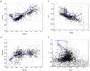 |
Fig. 2 Strömgren diagnostic diagrams obtained from deep STELLA/WiFSIP uvbyβ photometry. a) De-reddened color-color diagram (u−v) versus (b−y); b) color difference c1 = (u−v)−(v−b) versus the blanketing difference m1 = (v−b)−(b−y); c) Hβ index versus b−y color; d)V magnitude versus de-reddened color difference c1. The line is the 890 Myr isochrone with solar metallicity. The light-gray dot would be a Sun in IC 4756. We note that in panels a)–c) only stars with photometric errors smaller than ≈0 |
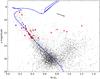 |
Fig. 3 Color−magnitude diagram constructed from STELLA/WiFSIP uvby photometry (small black dots). The best-fit isochrone from PARSEC (Bressan et al. 2013) with solar metallicity is overlaid. The filled symbols are the cluster members from our CoRoT sample from Table 1, while the open symbols are the CoRoT non-members. Triangles indicate binaries, blue (dark-gray) symbols moreover indicate the pulsating stars. The single green (light-gray) dot is the Sun. Nine of the CoRoT targets (#33, 32, 24, 23, 22, 20, 19, 12, 9) appear not to be cluster members. We note that the only cluster giant in our CoRoT sample is HSS 314 (#2; red filled triangle on the giant branch), which itself is a spectroscopic binary. The black arrow indicates the reddening vector. |
An 88-ks ROSAT HRI exposure initially yielded a detection of only a single cluster member (HSS 201 = BD+05°3863; Randich et al. 1998). This target is an A8 star with an X-ray luminosity of 7.3 1029 erg/s, and is not on our cool-star observing list. Reanalysis of the same exposure by Briggs et al. (2000) yielded four more sources, but with unknown cluster membership. A study of the rotational velocities in IC 4756 by Schmidt & Forbes (1984) also focused on A stars as these types populate the turn-off point. None of these targets matches the targets studied in the present paper.
3.2. Cluster membership of the CoRoT stars from radial velocities
Mermilliod et al. (2008) determined the average cluster velocity from 23 stars to be –25.15 km s-1 with a spread around the mean of approximately ±3 km s-1 peak to valley. This value is on the CORAVEL zero-point system (Famaey et al. 2005). Unfortunately, none of their 23 stars is within our CoRoT/SES sample. However, the STELLA/SES zero point was recently determined to be +0.503 km s-1 in the sense STELLA minus CORAVEL (Strassmeier et al. 2012). The STELLA/SES cluster mean velocity from 21 members is −24.0 ± 1.3(rms) km s-1 (all velocities in this paper are on the STELLA scale if not otherwise mentioned and given for barycentric Julian date).
Table 1 lists our averaged velocities and their standard deviations for the CoRoT stars. With the exception of the few bright targets (V ≈ 10m), all stars are at the S/N-ratio limit of the 1.2-m STELLA SES system. For the stars in the V range 10m−12m, we obtain RV residuals of typically between 50−300 m s-1 while for stars fainter than 12m this increases to ≈0.5−1 km s-1, always depending on the line broadening. Therefore, we emphasize that our systematic synthetic-spectrum fitting of all SES spectra with PARSES also comes with larger than typical errors because of the low S/N. Fifty echelle orders of each SES spectrum are selected for the fitting with the following four free parameters; Teff, log g, [Fe/H], and rotational line broadening vsini (for a more detailed description see Strassmeier et al. 2012 or Jovanovic et al. 2013). Additional spectral information, if reliable due to the low S/N ratio, is given in the individual notes.
Five CoRoT targets (#20, #19=HSS 185, #23=HSS 89, #24=HSS 198, #9=HSS 356) in the CMD in Fig. 3 do not fit into the cluster sequence at all. These stars appear too red in b−y by 03−10 for their brightness and are consequently judged to be either non-members or to be severely affected by intervening inhomogeneous dust clouds. Because their RVs are also significantly off the cluster mean, we are confident that none of them is a cluster member. Four more target are less discrepant ( ) to the CMD main sequence but still show far too low a RV to be considered cluster members. These nine stars are indicated in Fig. 3 as open symbols. See the individual notes in the appendix.
3.3. Reddening, distance, metallicity
The dark nebula LDN 630 is very close to IC 4756 at RA 18 38.9 and Dec+06 03 (Dutra & Bica 2002). Although not exactly in the line of sight, some of the peripheral regions of the nebula affect the colors of IC 4756 stars in the WiFSIP frames. The dust maps of Schlegel et al. (1998) indicate a very large average reddening of  (
( ) at the central position of IC 4756 compared to the obtained by Herzog et al. (1975) and
  by Schmidt (1978). The NASA/IPAC dust maps show a patchy absorption pattern across the cluster area which is also nicely seen in the WISE images4 at 4.6 μm and 12 μm. Our uvby photometry is compatible with the
  value. With a reddening of
  no agreement between our photometric data and standard evolutionary tracks can be achieved. This suggests that most of the dust in the IPAC and WISE data is located behind IC 4756.
The only prior Strömgren photometry is from Schmidt (1978). He noted that the calibration of his four-color photometry in terms of an absolute zero point was not always applicable to IC 4756, most likely because of foreground dust lanes likely related to the outskirts of LDN 630. We adopted standard stars from the compilation of Hauck & Mermilliod (1998) and found only a total of eight stars within our field of view suitable for a zero-point calibration of the STELLA/WiFSIP data. The standard uvbyβ transformation was applied by following the procedure given in Balog et al. (2001, and references therein). The equations are given in Appendix A. The best value for the reddening is  and the distance modulus
  . This equates to
  in the Johnson system. For the calibration of our measured β-indices the eight stars were only of marginal use because of their strong correlation with (b−y). The final results for the CoRoT targets are listed in Table A.2.
Figure 2a shows the de-reddened u−v vs. b−y color−color relation. Only stars with photometric errors below  are plotted, i.e., stars brighter than V ≈ 17m. Some of the scatter is also due to the lack of very cool standard stars in our color-color calibration. For M dwarfs (
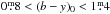 ), we see a large difference with respect to the solar-metallicity isochrone in the sense that the M dwarfs appear too bright in the ultraviolet by 02. However, almost all of these stars are non-member foreground stars.
Figure 2b plots the de-reddened color difference c1 as a measure of the discontinuity of the continuous hydrogen absorption vs. the de-reddened blanketing difference m1 for the same sample of stars as in Fig. 2a. For our cool stars, c1 is actually a measurement for absolute magnitude and surface gravity while m1 is a measure for metallicity. The homogeneous pattern in the figure suggests that these stars are indeed mostly cluster members while the stars significantly above and below the pattern are likely foreground or background stars. The relations in Holmberg et al. (2007) are used to determine individual metallicities for the validity range  . The average metallicity from 19 members of −0.19 ± 0.3 (Table 2) is basically consistent with solar metallicity. However, its scatter of 0.3 dex indicates the inhomogeneity of individual stars. The average metallicity of 9 members from spectrum synthesis is −0.13 ± 0.09, while the isochrones give equally good fits for a large range of metallicities peaking near solar values. While the grand non-weighted average from spectroscopy and photometry is −0.08 ± 0.06 (rms), the average from the CMD-fitted metallicities is −0.03 ± 0.02 (rms). We consider both values consistent with solar metallicity.
Figure 2c employs the Hβ index defined as the brightness difference in the narrow-minus-wide filters for the same sample as in Fig. 2a. It basically measures temperature for the stars cooler than spectral type ≈A2 ( ). While b−y also defines the temperature scale but is not free of blanketing, the Hβ index is additionally independent of interstellar reddening. We again apply the relations in Holmberg et al. (2007) to determine effective temperatures and absolute magnitudes.
Figure 2d shows V brightness vs. the de-reddened color difference c1. It is an observational H-R diagram. We note that we transformed y to V with the relation in Olsen (1994) for more convenient comparison with other clusters, and also extended the plotting range to V ≈ 20m. Almost all of the stars in the range 18–20m are background stars and only one of the fields has been plotted (because the region would appear black otherwise). We note that a Sun in IC 4756 would appear at V ≈ 14m (gray dot). The lack of bright evolved stars is compatible with the intermediate age of 890 Myr. The isochrone very well fits the 10 giants in Fig. 3 that were already identified by Schmidt (1978) and which are also part of the WiFSIP data.
3.4. Cluster age
Our main CMD from the STELLA WiFSIP photometry is shown in Fig. 3. The error level in y is on the order of mmag for stars brighter than 13th magnitude and up to for stars near 16th magnitude. The error level is larger by up to a factor of two for b and v as well as for u. The small dots in Fig. 3 indicate the WiFSIP stars and the big dots indicate the CoRoT stars. For the plot, we did not remove any of the non-members from the CoRoT sample but number specific outliers for identification purposes.
A main-sequence turn-off age is determined by fitting an isochrone from PARSEC (Padova models; Bressan et al. 2013). PARSEC is a stellar evolution code with up-to-date physics for post- and pre-main-sequence stars, with particular emphasis on chemical mixture and its relation with physical properties like the opacities and the equation of state. Its abundance scale has been adapted to the new solar chemical abundances with a solar metallicity of Z = 0.0152. Isochrones are provided for several photometric systems and for a large range of ages and metallicities. Colors are based on calibrations from ATLAS-9 spectra (Castelli & Kurucz 2003). Small but systematic differences are not surprising and are partly due to the isochrone calibration itself (see Clem et al. 2004).
No targets fainter than  were included in the isochrone fit owing to the increasing contamination with background stars. Figure 3 shows the best-fit isochrone with an overshoot parameter of 0.5, a formal cluster metallicity of [Fe/H] = −0.05 (which we deem still solar), a distance modulus
  , and for a reddening of
  . No particular isochrone gives a perfect fit in all colors. This is not unexpected given the small number of members and the lack of a well-developed giant branch at that age. The isochrone fit to the CMD from by data show the least rms error, and is consistent with the CMD from ub. The vy-CMD fit does not converge and thus would blur the age determination and is rejected. We note that the external errors of our CCD photometry for stars fainter than 16th magnitude would add to the general uncertainty and these stars are also not considered here. Such challenges (and other observational ones) in determining ages of open clusters were recently reviewed by Jeffery (2009) and we refer to this paper for further discussion. We infer a best-constrained age of 890 ± 70 Myr from our by data. The turn-off mass for IC 4756 is near 1.8 M⊙ (
 ; mid-A stars). Table 2 summarizes the various results from the CMDs.
Metallicity and age results.
4. Global rotation periods from CoRoT data
4.1. Periodogram technique and application
The detection of stellar rotation periods was accomplished in three different stages. The first stage was the calculation of the Fourier autocorrelation function (ACF). As demonstrated by Aigrain et al. (2008) and McQuillan et al. (2013) the first side lobe of the autocorrelation-spectrum serves as a rough estimate for the stellar rotation period and an initial error estimate. While this method proves to be very reliable for periods of several days, it is often difficult or impossible to determine a local maximum below one day lag. The second step consists of calculating the Lomb-Scargle (L-S) periodogram. Lomb (1976) proposed to use least-squares fits to sinusoidal curves and Scargle (1982) extended this by deriving the null distribution for it. We use the formulation implemented by Press et al. (2002) and compute false alarm probabilities following Frescura et al. (2008). The previously determined period from the autocorrelation is taken as a constraint. In case of a mismatch of both periods, a verification is done visually. As a last step a sinusoid is fitted to the light curve with the previously determined period in order to obtain a time-average amplitude. The final error estimate for the period was obtained through Bayesian testing; the signal with the best-determined period was removed from the light curve and an artificial signal at random periods was injected and its period then measured with the same procedure.
4.2. Rotation vs. pulsation and binarity
The resulting periods and amplitudes are given in Table 3. The derived periods range from 0.15 d for star #12 to 11 d for star #36. The average amplitudes in Table 3 are only guidelines because amplitude variations are the rule and typically span a factor of 2–3 over the time-span of the observations. We note again that the light curves were normalized and linear trends removed. This effectively prevents any statement regarding multi-periodic behavior with periods longer than ≈1/2 of the length of the data set (≈40 days for LRc06).
Five systems (#5, 6, 10, 12, 13) are non-radial pulsators with rather short fundamental periods (P< 0.8 d). These are obvious in the light curves shown in Fig. 1; these systems exhibit many more periods than just the one listed in Table 3. Two additional systems (#15, 22) show very stable light variations over the time of observation and are classified as close binaries. Star #15 (HSS 348) additionally shows narrow eclipses and is therefore actually a triple system.
Photometric periods from the CoRoT data set.
4.3. Evidence of differential rotation
The analysis of differential rotation in the light curves is based on two tools, basically the ACF already mentioned and a Fourier analysis with a fast Fourier transform (FFT). Narrow frequencies or periods cannot be resolved at lower frequencies in the power spectrum, but are visible as a beat frequency in the ACF. Usually, two narrow periods are identifiable after five to ten cycles in the ACF as two separate peaks, where their maxima can be determined. We identify them as the side-lobes in the FFT and use a least-squares spectral decomposition (LSSD) to find the best period for the targets with side lobes. These periods are listed in Table 4 and supersede the periods in Table 3 from the ACF despite that the error bars are in some cases larger.
Six targets show a frequency splitting in the L-S periodogram at the rotational frequency. Figure 4 shows the frequency splitting for the six stars and compares them with a representative target (#11) where no splitting is detected. We plot period on the x-axis in Fig. 4 in order to compare with other periods in Table 4. We interpret the splitting to be due to differential surface rotation and convert it into radians per day. Numerical values in terms of ΔΩ/Ω are between 0.044 and 0.15 and compare to the solar value of 0.2. Its errors are the quadratically summed relative errors from the individual periods. Three additional targets (#9, 36, 38) had unusually extended side lobes so that we tend to interpret them to be dominated by shot-term spot evolution rather than differential rotation. It is worth mentioning that the six targets in Table 4 show always more than just one side lobe which we interpret as evidence of spots at more than just two latitudes.
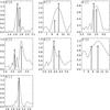 |
Fig. 4 Stars with evidence of differential surface rotation. Shown are relative amplitude vs. period in days of the stars in Table 4. The main periods are indicated with dots and dashes. Star #11 is a comparison star where no differential rotation is evident. |
5. Orbital elements
Eleven of our bona fide IC 4756 members turned out to be spectroscopic binaries (identified in Table 1). One binary has been known previously (HSS 314 = #2); the others are new detections. For six targets, we have enough velocity measurements to principally solve for the usual orbital elements of a spectroscopic binary (three of them being preliminary owing to the poor phase coverage). Radial velocities were determined from a simultaneous cross-correlation of 62 échelle orders with a synthetic spectrum matching the target properties as far as known (see Weber & Strassmeier 2011 for a detailed description). We apply the general least-squares fitting algorithm MPFIT (Markwardt 2009) and refer to Strassmeier et al. (2012) for computational details. Table 5 summarizes the orbital elements for these six targets and Fig. 5 compares the observations with the predicted elements.
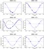 |
Fig. 5 Radial velocity variations and orbital solutions for the six stars in Table 5. We note the preliminary character for the orbits for HSS 314, 174, and 189. |
STELLA orbital solutions. Column “rms” denotes the quality of the orbital fit for a measure of unit weight in km s-1.
Six of the 11 targets are double-lined spectroscopic binaries. One target, HSS 106 (#4), appears double lined at first glance but one line system appears constant while the other varies sinusoidally (see individual notes). It is thus a single-lined spectroscopic binary. HSS 174 (#17) is a similar case with a broad-lined spectrum whose RVs are used to determine a preliminary SB1 orbit. Its narrow-lined spectrum appears to be constant. Another target, HSS 108 (#5), shows RV variations of up to ≈18 km s-1 but is also a pulsating star and the RVs are only marginally consistent with orbital variations as its pure cause. We computed a hypothetical orbit from the current data but list it only in the individual notes for guidance.
6. Hα photometry and spectroscopy
6.1. Photometric filter definition
In order to access a magnetic activity tracer in as many cluster stars as possible, we performed Hα wide- and narrow-band photometry with STELLA, where WiFSIP is equipped with Narrow-band (FWHM 4 nm) and wide-band (FWHM 16 nm) Hα filters. A total of 356 CCD frames in all fields were obtained and stacked to create a deep Hα image across the cluster reaching an equivalent V brightness of ~20th mag. We follow the annotations of Herbst & Layden (1987) and determine a N−W (narrow minus wide) α index from this photometry from 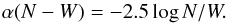 (1)In Fig. 6a, we plot the internal errors for approximately 7000 targets from the stacked CCD image. Their formal standard errors range from 0.1−0.2 mmag for the brightest targets (V brighter than 10 mag) to about 01 for the faint limit near V ≈ 20 mag.
6.2. An activity H–R diagram for IC 4756
At the age of ≈900 Myr, we do not expect much magnetic activity left from the early stage at the ZAMS. We know from the Hyades that the magnetic brake has already efficiently slowed down the rapid rotators at its 625 yr age and thereby effectively switched off magnetic activity. The 11 targets in IC 4756 with large amounts of surface lithium are all verified to be definite cluster members. Surface lithium is a sign of either youth and/or some rotation-induced extra mixing. Unsurprisingly, 3 of the 11 Li stars are close binaries while two additional ones are possible binaries with high rotation rates. None of the Li stars is a giant.
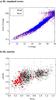 |
Fig. 6 Hα photometry of IC 4756. a) Standard errors in the STELLA Hα CCD data for both filters (n narrow, w wide). b) Hα index α versus de-reddened b−y color; an activity analog of the H–R diagram. Hα emission increases upward, Hα absorption increases downward. The thick dots indicate the CoRoT stars from Table 1. Spectral type and color equivalents are dF0, |


Figure 6b shows the α index as defined in Eq. (1) as a function of b−y. This diagram is an activity analog of the H–R diagram because most of the targets form a main sequence which itself is split into a convection-dominated and a radiation-dominated part. The latter is characterized by the change of the strength of the Hα line with effective temperature and whether its formation is photo-ionization dominated or collision dominated. Brighter α index in Fig. 6b means more emission while fainter α index means more absorption. Stars with pure (chromospheric) emission lines will lie above the main sequence, e.g., the active M dwarf sample of Herbst & Layden (1987).
The homogeneity of the points in Fig. 6b indicates that IC 4756 is a magnetically quiet cluster containing no significantly active stars, except perhaps in close binaries. As such it resembles the Hyades. However, IC 4756 has ≈10 giants whereas the Hyades is known to have just four which is in agreement with IC 4756 being slightly older than the Hyades. The sample of CoRoT stars in this paper identifies only one cluster giant which is a spectroscopic binary with a period of 6.8 yr (HSS 314; Table 5). See also our individual notes.
6.3. Equivalent widths and index calibration
Because all of our CoRoT targets have at least one high-resolution échelle spectrum, we also attempt to verify the photometric α index with a spectroscopically measured equivalent width (EW). The Hα index is a dimensionless and non-physical quantity, and is thus not directly comparable to spectroscopic studies that usually measure an equivalent width in mÅ or a relative surface flux in erg cm-2 s-1. The only shortcoming with our calibration of α vs. EW is the low S/N of most of the spectra. We also expect some intrinsic Hα variability for some of these targets but this effect is expected small compared to the measuring errors, in particular at the given cluster age.
Hα equivalent width is defined as the flux below the continuum absorbed by the full Hα line profile. The targets in Table 1 exhibit rather different profiles ranging from wing-dominated hot dwarfs to wing-less cool giants. The latter, though, are mostly cluster non-members. We employ the splot routine in IRAF for the measurement and use a Lorentzian profile fit. Repeated measurements of one and the same spectrum allow an estimate of the internal error. It is dominated by the low S/N ratio and only to a much lesser extent by the fitting function and procedure. Repeated measurements when a target has more than just a single exposure allow an estimate of the external error. In our spectra the external error is driven by the uncertainty of the continuum level and is typically 10–20%. For the faintest targets it may amount to 30% (after all, these are R = 55 000 spectra of 13th-mag stars with a 1.2 m telescope).
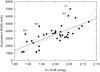 |
Fig. 7 Photometric Hα index N-W (narrow minus wide) in magnitudes vs. spectroscopic Hα equivalent width in milli Angstroem. The line is a simple regression fit and the dotted lines are its 95% confidence levels. Four outliers are identified and discussed in the text. |
Figure 7 shows the relation between the photometric α index and the spectroscopic equivalent width. A linear regression appears to be an adequate fit and is  (2)The standard deviation is 680 mÅ. Four stars lie significantly above the bulk (#1, 29, 31, 34). Star #1 is a very broad-lined A star with an uncertain continuum setting, #29 has very narrow lines but very extended Hα wings, #31 is a SB2, and #34 is our extreme flare star. If removed from the sample the reduced standard deviation is close to 550 mÅ. There is a color dependency of Hα EW with b−y which peaks at early A stars (
 ) and contributes to the residuals of the fit from Eq. (2). A linear regression with Strömgren b−y from the same sample of stars gives the functionality
  (3)
(3)
6.4. Lithium abundances
A total of 12 cluster members show a Li i λ670.78-nm absorption line. Eleven are early-to-mid G dwarfs, one is a late-G or early-K dwarf. Lithium on the surface of cool main-sequence stars is usually interpreted to be a sign of youth and/or an enhanced mixing process possibly because of the presence of rotation and a magnetic field or the engulfing of a Li-rich large planet. We have two targets in our sample (#36, #37) in common with the three targets measured by Pace et al. (2010). Their spectroscopically determined effective temperatures and metallicities differ to ours by up to 300 K and 0.1 dex, respectively, while the lithium abundances are in reasonable agreement. We emphasize that our spectra are of comparatively low S/N.
Lithium abundances in this paper are determined from the equivalent width and the effective temperature from the spectrum synthesis with the aid of the NLTE conversions from Pavlenko & Magazzu (1996). Spectra have S/N ≈ 20−50:1 but multiple spectra allowed a repeated detection which was used to verify the Li i-line. The nearby Ca i 671.7-nm line was measured for comparison and its numerical values are given in the individual notes. A Gaussian fit or, if the S/N was very low, a simple line integration yielded the individual equivalent widths for the combined lithium isotopes. The equivalent width of the Fe i 670.74 blend was taken from the NSO solar atlas (Wallace et al. 1998) and subtracted from the measurements. It is given in the individual notes. The time averaged Li results are listed in Table 6. Abundances are with respect to the log n(H) = 12.00 scale for hydrogen.
The IC 4756 G-dwarfs have an average NLTE Li abundance of log n = 2.39 ± 0.17(rms). The Li abundance for the SB2-primary HSS 174a (# 17) is just a lower limit because the errors in the temperature (and the gravity) are very large (800 K, 0.5 dex). Another target (HSS 95=#16) shows Li i-670.8 at the 50 mÅ level but its Teff determination is not reliable (see individual notes).
Cluster members with lithium detection.
7. Summary and conclusions
We have reported deep wide-field photometry of the open cluster IC 4756, together with time-series photometric and spectroscopic monitoring of 38 brighter stars in the region of the cluster. IC 4756 is particularly interesting because it is comparable in age with the Hyades. We have revised the cluster age to 890 ± 70 Myr and have determined an average reddening E(b−y) of 016, a distance modulus of 802, and an average metallicity of –0.08±0.06. At this age of IC 4756, we do not expect rapid stellar rotation anymore and thus no (or only marginal) magnetic activity. This is confirmed by our Hα photometry and spectroscopy, which also led to a calibration of the photometric Hα index with spectroscopically determined equivalent widths.
CoRoT photometry of 37 of the 38 targets enabled us to determine precise periods for 27 of them. Five stars with periods less than a day are all non-radial pulsators with a rich and complex frequency spectrum. The shortest rotation period is 1.68 d for the late-F star HSS 95 and the longest is 11.4 d for the G2-dwarf HSS 240. For six of the rotating stars, we see a splitting or asymmetric broadening of the main frequency and use this to determine surface differential rotation. Values of ΔΩ/Ω between 0.04 and 0.15 rad d-1 show them to have generally weaker differential rotation than the Sun. Eleven G-stars were found with an average logarithmic lithium abundance of 2.41 ± 0.17 (rms), almost identical to the G dwarfs in the Hyades (see Takeda et al. 2013). Two of these targets are double-lined spectroscopic binaries where both G-components show a lithium line. In addition, ten new spectroscopic binaries were found in this paper and orbits have been presented for five of them. In a forthcoming paper, we will extend our CoRoT sample for IC 4756, and aim to construct a color-period diagram.
Online material
Appendix A: STELLA/WiFSIP observing log, transformation functions, and combined CCD images
 |
Fig. A.1 STELLA/WiFSIP fields for IC 4756. Six fields were observed, indicated by the dashed boxes. Field f2 in the top left corner had been offset due to an intervening bright star. Each field is 22′×22′ and the total coverage is 0.67 sq. deg or 38% of the cluster. The approximate size of the cluster (90′) is indicated by the large circle on the left. The cluster center is at 18h38m31.2s, +05°29′24′′ (2000.0) and is highlighted by the rotated square box. The stellar ID numbers are the running numbers from Table 1 and identify the stars observed with CoRoT. The image is a uby composite. |
Table A.1 is the observing log of the Strömgren photometry with the Wide Field STELLA Imaging Photometer (WiFSIP). Only observing blocks are identified, not the individual CCD frames. One observing block consists of five consecutive integrations in u, v, b, y, Hαn, Hαw, Hβn, and Hβw. The table lists the mean JD given for the mid exposure, the field identification from Fig. A.1, the total number of CCD frames, total exposure time, the FWHM of the average stellar image, and the average airmass of the block.
The transformation equations are based on the calibration of Crawford & Barnes (1970) and we followed the recipe from Balog et al. (2001). Its four zero-point constants refer to the slopes for (b−y), m1, c1 and β, respectively, while the three color-term coefficients are for V, m1 and c1. The WiFSIP field of view contained eight standard stars from the compilation of Hauck & Mermilliod (1998) and six of them could be used to determine the zero points. However, all of these stars are brighter than 9th magnitude in V and are thus close to the saturation limit of our CCD. Therefore, the standard deviations between the literature values and the WiFSIP instrumental values are comparablylarge, ± 0.012 for (b−y), ±0.07 for c1, ±0.04 for m1 and ±0.19 for β, and are not representative for the photometric precision. The (b−y) color term in the equations for m1 and c1 was too uncertain and was set to zero. 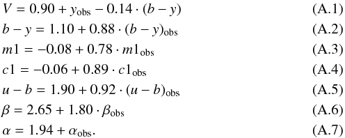 A.1The final WiFSIP Strömgren and Hα indices for the CoRoT stars are listed in Table A.2.
The epoch stacks were astrometrically re-calibrated in the tangent plane projection with distortion polynomials using sources detected in Johnson H or Ks from the 2MASS catalog (Cutri et al. 2003), and those with Johnson  . An IRAF script iteratively invokes CCFIND, which correlates the catalog sources with those in the image, and CCMAP, which computes the astrometric solution. The Legendre fit to the projection transformation was cubic, with a threshold of 2.4 σ to reject outlier astrometric points. The resulting projection transformation had a standard deviation typically of ≲0.10′′ in both right ascension and declination.
STELLA/WiFSIP observing log.
The combined images for each bandpass represent very deep integrations with an equivalent exposure time of, e.g., 3900 s in y and up to 10 740 s in narrow-band Hα. Thereby, the IRAF FINDSTAR routine identified the following numbers of stars per CCD field in the y band: f2 29 102; f3 16 152; f5 16 302; f6 19 607; f8 22 870; and in f9 18,758 stars. The 5σ limiting magnitude in y is 21 mag. Aperture photometry was then performed with the IRAF daophot routine with apertures adapted to the FWHM of the frame under the requirement of optimal sampling. Average internal errors are basically photon-noise limited in all bandpasses and reach 1 mmag for stars between 125–135 and 02 at the limiting magnitude in y. These rms values are obtained relative to a sky background in the immediate vicinity of the numerical aperture. External errors are estimated from the rms of all combined nightly frames.
Results from STELLA/WiFSIP Strömgren photometry.
Appendix B: Notes on individual targets
HSS 73 = #1
The CoRoT photometry in imagette modus is overexposed and consequently the relative brightness amplitudes are rather uncertain and are only for orientation. The periodicity of 0.4 d of the light variations should not be affected, but the amplitude is so close to the noise that we are uncertain about its reality and dismiss it. The value in Table 3 is thus very tentative. The spectra are those of a mid A-star with very broad Balmer lines with equivalent widths up to 20 Å for Hα, 14 Å for Hβ, and 10 mÅ for Hγ. Our RVs are only estimates. The diffuse interstellar band (DIB) lines at λ661.3, 578.0 and 579.7 are clearly detected and match those of other cluster members (λ862.1 is not detected).
HSS 314 = #2
Thirtynine RVs confirm this star (also designated Kopff 139) to be a long-period SB1. An orbit was published earlier by Mermilliod et al. (2007) with a period of 3834 ± 36 d (10.5 yrs), an eccentricity of 0.22 and a K-amplitude of just 2.6 km s-1. Our data span a full amplitude of 4.4 km s-1 already within 843 d (2.3 yr) and it is thus possible that above orbital period is wrong. However, our data are not sufficient in coverage yet to compute a definite revised orbit but a preliminary circular orbit from STELLA data alone is given in Table 5 with Porb = 2487 d (6.8 yr). PARSES finds the best fit with Teff = 5070± 50 K, log g = 3.8 ± 0.1, vsini = 3.9 ± 0.3 km s-1, and [Fe/H] = −0.16 ± 0.03.
HSS 138 = #3
The Balmer lines appear broad with equivalent widths of 3.5 Å for Hα, 3.0 Å for Hβ, and 3.0 mÅ for Hγ. The interstellar Na D lines are sharp and very prominent. Radial velocities are difficult owing to a lack of spectral lines. The wavelengths with respect to the DIB lines are in agreement with the expected cluster velocity and we are confident that the star is a member. A PARSES solution of the best spectrum suggests Teff = 6900 K, log g = 3.5, vsini = 100 km s-1, and [Fe/H] = –0.45 which suggests either a late-A or a slightly evolved mid-F star.
HSS 106 = #4
The star is a single-lined spectroscopic binary with an orbital period of 23 d (Table 5). We sometimes see a double-lined spectrum due to a third star whose velocities appear constant. It is unclear whether this star is a background or confusing source or part of a long-period triple system. No clear photometric period could be extracted from the CoRoT photometry.
HSS 108 = #5
Pulsating star in a single-lined spectroscopic binary. We have 40 RVs that suggest a low-amplitude of just 4 km s-1 with an orbital period of 25.7 ± 0.15 d. The orbit is so uncertain that we want to mention it only in these notes (other elements are T0 = 2 456 391, γ = −13.5 ± 1 km s-1, e = 0, a1sini = 1.42 ± 0.29 × 10⁶ km, and f(M) = 0.0002 ± 0.0001). The fundamental pulsation period is 0.438 d.
HSS 113 = #6
The Balmer lines appears very broad with equivalent widths of 4 Å for Hα, 2.9 Å for Hβ, and 3 Å for Hγ. The interstellar Na D lines are sharp and prominent. The target is an A–F star with vsini of ≈250 ± 50 km s-1. The star pulsates with a period of 0.353 d which is likely the fundamental pulsation period in a Delta Scuti-type star. Therefore, RVs are very difficult to obtain and we judge the value of −10 ± 4 km s-1 to be still in overall agreement with the cluster mean.
HSS 112 = #7
The STELLA RVs do not allow a membership statement. The target has broad Balmer lines suggestive of vsini of ≈150 ± 20 km s-1. However, no pulsation pattern like in HSS 113 is seen. The periods from the CoRoT light curve are ambiguous, a FFT gives a 14-d value while the ACF suggests ≈40 d.
HSS 107 = #8
Double-lined spectroscopic binary of two nearly equal components. An orbit with Porb = 11.65 d is given in Table 5. Na D has a strong interstellar absorption component and is partly affected by geocoronal emission. Both components show a Li i λ670.8-nm line with an equivalent width of 80 ± 4 mÅ compared to 110 ± 5 mÅ for the nearby Ca i 671.7 line (both values corrected for two equal continua). Line ratios in the 640-nm region suggest an early-G spectral type and convert the Li equivalent width into an abundance of log n ≈ 2.5 (NLTE) under the assumption of Teff,1 = Teff,2 = 5700 K. We measure vsini for both components of 4.5 ± 1.5 km s-1.
The CoRoT data gave uncertain but consistent photometric periods from a FFT (10 ± 0.5 d) and from the ACF (11 ± 0.5 d). The average is adopted in Table 3.
HSS 356 = #9
Not a cluster member. The SES spectra show it a K5III giant with an average RV of –19.3 km s-1, almost a perfect match with the M-K standard α Tau. The Balmer lines appear as narrow absorption lines without noticeable wings. Optically thin lines appear also sharp with only small rotational broadening of vsini = 4.5 ± 0.5 km s-1. No Ca ii H&K nor IRT emission nor Li i 670.8-nm or He i 587.5-nm absorption is detectable. The star is thus not chromospherically active. The red to near-IR part of the spectrum is dominated by molecular lines, e.g., the typical TiO bandheads, e.g., at 705.5 nm. The Na D doublet appears very asymmetric with a broad wing only on the respective blue-wavelength sides but sharp on the red sides. This is due to a stationary emission component redshifted by +43 km s-1 that is also seen at Hα and K i 769.9 nm where it appears with a redshift of ≈42 km s-1. The DIB line at λ661.3 nm has an EW of 180 mÅ. The forbidden oxygen lines from [O i] at 557.7, 630.0, and 636.4 nm appear with line intensities relative to the continuum of up to 5, 0.5, and n.d., respectively, and are all mostly of geocoronal origin.
Our PARSES analysis suggests an effective temperature of 3890 ± 50 K and log g of 1.4 ± 0.5. The large error in the metallicity, –0.01 ± 0.22, indicates cross talk in the solution with log g, and thus it is likely that both values are not real. The expected absolute magnitude of a K5 giant is –02 ± 0.2 and its distance modulus is ≈117. Thus, the star is in the cluster background at ≈1.9 kpc.
The CoRoT light curve clearly indicates changing variability with an amplitude of up 015 and a period of 4.25 d. The FFT reveals three discrete peaks at 4.257 d (main peak) 5.253 d and 3.629 d. The FWHM is 0.21 d and the formal ΔΩ/Ω would be 0.782 ± 0.003. The highly variable and modulated light curve and the three isolated periods along with a highly variable ACF could either indicate three different active longitudes or systematic spot evolution. When P is interpreted as the rotational period of the star the minimum radius Rsini would only be 0.38 R⊙. Furthermore, if we assumed a radius typical for a K5 giant of 25 R⊙ the inclination would be below 1°. We note that the K5III MK-standard α Tau has a measured radius of 44 R⊙ (Richichi & Roccatagliata 2005). In any case, it is highly unlikely that the 4.25-d period is the rotation period of the K5 giant but could stem from a very close-by undetected and large-amplitude foreground star.
HSS 241 = #10
Pulsating star with 0.8-d fundamental period. Six RVs, evenly distributed within two months in 2013, show a steady decrease from –11.4 to –25.6 km s-1. It suggests a SB1-binary with yet unknown systemic velocity. The RV in Table 1 is a current average. The DIB lines at λ661.3, 578.0, and 579.7 are of comparable strength than for cluster members.
HSS 269 = #11
It appears that our STELLA SES data base of HSS 269 consists of three different stars. One target was a plain misidentification (HSS 279; not a cluster member, see below). The other target is a very close neighbor of comparable brightness (HSS 267, separated by 6.7′′). STELLA acquired the correct target in normal weather conditions but the guider may have accidentally picked up the close target during occasions of high wind gusts during at least three occasions. These data were removed but the overall rms of our RVs of HSS 269 remained larger than expected. In addition, CoRoT did not resolve the two targets and thus its photometry is always for both stars.
The STELLA spectrum 20130814B-0006 is for HD 172248 (=HSS 279) and shows a strong He i λ587.5 line with an EW of 160 mÅ. The two Si ii lines at λ634.7 and λ637.1 are measured with EWs of 182 mÅ and 150 mÅ, respectively. The entire spectrum resembles that of a B supergiant. The neutral potassium line K i 769.9 nm is detected with an EW of 40 mÅ and the O i-777 nm triplet is well resolved with a residual intensity of 0.75. However, no Ca ii irt lines are apparent nor do we see the hydrogen Paschen series although a very broad feature spanning the entire echelle order coincides with P12 λ875 nm. PARSES does not converge on a solution, which indicates parameters out of its range (which would be the case for a hot supergiant); vsini appears unmeasurable but the RV is –12.8 km s-1. The DIB lines at λ661.3, 578.0 and 579.7 are clearly detected with EWs of 98, 125, and 35 mÅ and appear stronger than those of cluster members. We conclude that HSS 279 is not a cluster member but a background early-B supergiant.
In comparison, the other two STELLA spectra obtained on April 8 and June 14, 2013 show a comparable but not identical spectrum to HSS 279, in particular the He i line is completely missing. The two Si ii lines appear weaker with EWs of 100 and 55 mÅ, respectively. The Ca ii irt lines appear weak but are clearly detected, and again no sign of the hydrogen Paschen series. Radial velocities are –23.9 and –20.6 km s-1 for the two spectra, respectively, which fit the cluster mean, and vsini is ≈13 km s-1. The DIB lines are detected but are much weaker than in the spectrum of HSS 279 and in agreement with the cluster distance. Hα is typical for a late-F dwarf in agreement with its (b−y)0 of 0316 from WiFSIP.
The combined CoRoT light curve of HSS 269 and HSS 267 shows a clear and modulated variability with a period of 2.0334 d. If indeed a late-F dwarf, this period is likely its rotation period due to spots.
HSS 208 = #12
Background star with strong DIB lines of 208, 420, 110 mÅ at λ661.3, λ578.0 and λ579.7, respectively. The Balmer and Paschen serie of hydrogen are dominating the spectrum (EW Hα 3.8 Å; EW Hβ 4.2 Å). The ISM Na D lines are saturated and the K i-769.9 line has an EW of 130 mÅ. The spectrum of this star is otherwise almost featureless. The CoRoT photometry shows an oscillation spectrum with a fundamental period of 0.154 d.
HSS 270 = #13
Pulsating hot star with very broad spectral lines. The O i triplet is not resolvable. In contrast, K i 7699/7665 as well as the Na D lines appear very sharp. The Na D lines reach basically zero intensity in the core. If these lines are of ISM origin then the target must be a background star. Then, the average RV of −22.2 ± 2.5 km s-1 must be a chance agreement with the cluster mean. Unfortunately, this part of the cluster is affected by intervening dust clouds as seen from the WISE images at 4.6 μm and 12 μm and thus the WiFSIP-based de-reddening may be inappropriate. Therefore, we cannot firmly conclude on its membership but removed the target from the isochrone fit.
HSS 57 = #14
The CoRoT data reveal two periods of 10.7 d and ≈1 d that are both seen by naked eye in Fig. 1. Our spectra indicate a He i λ587.5 absorption line with an EW of 120 mÅ. Both Na D lines are dominated by the sharp-lined ISM components. Si ii at λ634.7 and λ637.1 is measured with EWs of 120 mÅ and 50 mÅ, respectively. The He i line and the two Si ii lines indicate a hot star. The rest of the spectrum morphology suggests an early-G or late-F dwarf and the 10.7-d CoRoT period appears to be its rotation period. It is possible that the spectrum is a combination of two stars.
HSS 348 = #15
Double-lined spectroscopic binary with an eclipsing tertiary star.
HSS 95 = #16
The O i triplet at 777 nm appears blended but is clearly detected with a combined EW of 557 mÅ. The traces of Li i 670.7 are very weak due to the low S/N ratio but appears detected on an EW ≈ 50 mÅ level. Other spectrum tracers, like the Hβ, Hγ, Ca ii irt and many of the strong Fe i lines in the blue region, indicate a rapidly-rotating late-F star with vsini = 31 ± 4 km s-1 in agreement with the 1.68-d CoRoT period. A strong redshifted ISM line with EW of 90 mÅ is seen at K i 769.9 nm (and also at Na i D). The DIB line at λ661.3 has an EW of ≈75 mÅ.
The CoRoT light curve in Fig. 1 clearly indicates period doubling due to two migrating starspots. The full amplitude doubles from 5 mmag to 10 mmag from double-humped to single-humped light curves. The FFT has its main peak at 1.6754 d and a separated peak at 1.7628 d, another period may be real at 1.6096 d but is within the FWHM of 0.0785 d of the main peak.
HSS 174 = #17
Double-lined spectroscopic binary where the weaker component is narrow lined and the stronger component broad lined. The spectrum synthesis picks up only the stronger component and suggests a late-type star with Teff = 5000 ± 800 K, log g = 4.1 ± 0.5, and a vsini of 14 ± 2 km s-1. However, its solution is affected by the secondary lines. The metallicity is unconstrained in our fits. Vsini of the secondary is < 4 km s-1. We measure a Li i 670.8-nm line from the strong-lined component with an equivalent width of 47 ± 3 mÅ (compared to 60 ± 4 mÅ for the nearby Ca i 671.7 line). The spectrum morphology and various line ratios in the 643-nm region suggest two early-G stars with effective temperatures and gravities more near the upper limits of the PARSES results. We assume 5800 K and log g = 4.6 and a continuum ratio of 2:1 (primary to secondary) to convert above Li equivalent width into an abundance.
The FFT shows a single peak at 9.115 d and a smaller peak at 12.14 d. The ACF indicates periods at 9.357 d and 8.2475 d, with the lower period still within the FWHM of 1.86 d of the main peak.
HSS 185 = #19
The spectrum synthesis fits of five spectra consistently give Teff = 4700 ± 100 K, log g = 3.6 ± 0.3, [Fe/H] = +0.2 ± 0.1, and a vsini of 4 ± 1 km s-1. Its many sharp photospheric lines, the wing-less Balmer lines, and several line-depth ratios at 643 nm are in agreement with a K0-2 III-IV luminosity classification. The star is therefore not a cluster member. No measurable Li λ670.78 line is present (EW< 10 mÅ).
USNO-B1 0957-0380847 = #20
Not a cluster member. The PARSES effective temperature is 4,630 ± 100 K, log g = 1.5 ± 0.3 and [Fe/H] = −0.45 ± 0.1. Vsini is basically not measurable with a nominal value of 1 ± 1 km s-1. The interstellar Na i D lines appear very complex and very strong and are split into two broad complexes separated by 1.0 Å, very similar to star #23. The DIB line at λ661.3 has an EW of around 100 mÅ. The Hα profile shows no wings and appears typical for a giant. The star is in the background and is likely a K-type giant. No measurable Li λ670.78 line is present (EW< 10 mÅ).
HSS 194 = #21
Both Hα and Na D show a red-shifted, stationary, and sharp emission-line component. Its redshift is 48 km s-1 for both D lines and ≈48 km s-1 for Hα. The D2 emission appears much stronger (residual intensity of 1.4) than the D1 emission (residual intensity of around 1.0). Na D appears basically without wings and shows subtle line-profile structure most likely due to intervening interstellar absorption. The forbidden oxygen lines from [O i] at 557.7, 630.0, and 636.4 nm rise above the continuum with relative line intensities of up to 12, 5, and 2, respectively. We believe that all these emission lines are of geo-coronal origin.
The ACF shows a different signal after about seven variability cycles, i.e., after ≈ 23 d, with two distinct maxima of 3.33375 d and 3.51875 d. The two peaks are also visible in the FFT (Fig. 4 and we interpret them as due to two spots co-rotating at two different latitudes). The respective errors are estimated from the FWHM to be 0.13 d.
HSS 158 = #22
Probably not a cluster member. Close binary, likely an eclipsing β Lyrae-type system. Therefore, the period in Table 3 is the orbital period (which is likely also the rotation period because one would expect a bound rotation). The spectrum appears to be that of an A star. Five RVs show a range of –24 km s-1 to +21 km s-1. A single spectrum taken on Mar. 30, 2013 shows it with a sharp central hump in the Hα core, most likely due to the RV shift of the two stellar components. All spectra show the Paschen series until P12 at 875.0 nm. Strong DIB lines, e.g., at 6613 Å, also indicate rather a background target than a cluster member.
HSS 89 = #23
Not a cluster member. The PARSES effective temperature is 4560 ± 150 K, log g = 3.3 ± 0.1 and [Fe/H] = −0.02 ± 0.02. Vsini is basically not measurable with an upper limit of 2 km s-1. The interstellar Na i D lines appear very complex and very strong and are split into two broad complexes. The DIB line at λ661.3 has an EW of around 120 mÅ, but difficult to measure. The star is a background early-K giant. No measurable Li λ670.78 line is present (EW< 10 mÅ).
HSS 198 = #24
Not a cluster member. The spectrum-synthesis fits of five spectra consistently give Teff = 4 570± 110 K, log g = 2.5± 1.0, [Fe/H] = −0.2± 0.3, and a vsini of 2 ± 1 km s-1. The star seems to be a background K2 giant or subgiant with strong and complex Na D and K i line profiles. No Li λ670.78 feature greater than 10 mÅ is detectable. The 7-d period from the ACF could be an alias of a longer period. The Lomb-Scargle periodogram gave 7.215 ± 0.03 d with a smaller amplitude than ACF (4 instead of 6 mmag) but an almost equally strong second period at around 16 d.
HSS 209 = #25
Our PARSES converged on three of the five spectra with average values of Teff = 6060± 240 K, log g = 4.7 ± 0.2, [Fe/H]= −0.2 ± 0.2, and a vsini of 22 ± 4 km s-1. These parameters suggests an ≈F9 dwarf star. Five RVs outline a weak linear trend from –24.6 km s-1 in early May 2013 to –23.3 km s-1 by the end of August 2013 with an unweighted average of −23.9 ± 0.6 km s-1 (rms). The star could be a long-period binary but the RV evidence is not yet convincing. Strong red-shifted ISM lines at Na D and K i 769.9 nm dominate its profiles. The 3-day period in Table 3 is from a Lomb-Scargle analysis and is very uncertain, the ACF did not give a convincing period at all. Three days is nevertheless in agreement with the measured vsini and the expected radius of an F9 dwarfs and is thus most likely the rotation period of the star.
HSS 259 = #26
Five spectra indicate average values of Teff = 5200± 400 K, log g = 4.35 ± 0.25, [Fe/H] = −0.9 ± 0.5, and a vsini of 10 ± 2 km s-1. The star is a rapidly rotating late-G or early-K dwarf. A strong Li i-670.8 line is detected in all of the spectra with an equivalent width of 104 ± 6 mÅ (compared to 100 ± 6 mÅ for the nearby Ca i λ671.7 line). We subtracted an equivalent width of 6 mÅ from above value to obtain the logarithmic abundance of log n ≈ 2.2 in Table 6. The light curve shows occasionally repeated dips that indicate a 5.9-day period, but overall it is not well defined and must be judged preliminary. However, a 5.9-d period is in fair agreement with the vsini and the radius of a late-G dwarf.
HSS 284 = #27
The ACF indicates two close periods at 3.8051 d and 3.8688 d. The FFT periodogram shows only one peak at 3.867 d with a FWHM of 0.3 d. The LSSD revealed two comparable periods of 3.874 d and 4.346 d. Four RVs show a linear change from –22.2 to –24.6 km s-1 within two months in 2013 indicative of a long-period SB1-binary. The spectrum morphology and two PARSES solutions suggest an effective temperature of 5700 ± 200 K, log g of 4.6 ± 0.1, [Fe/H] = −0.23 ± 0.2 and vsini = 13± 3 km s-1. The star is a rapidly rotating early-G dwarf. A Li i-670.8 line is detected in one of the spectra with an equivalent width of 46 ± 3 mÅ (compared to 81 ± 4 mÅ for the nearby Ca iλ671.7 line).
HSS 189 = #28
Double-lined spectroscopic binary. Table 5 gives a preliminary orbit based on 8 respective 6 measurements. The period of 110 d is accordingly uncertain. No Li i-670.8 lines detected. The spectrum morphology around the λ643-nm region suggests two mid F-dwarf stars. The ACF period of 7.2 d might be spurious. A Lomb-Scargle periodogram gives three equally strong peaks at 12.15 d, 6.73 d and 5.27 d but with smaller amplitudes than the ACF period.
HSS 211 = #29
An early G-dwarf star. PARSES solutions for five spectra suggest Teff = 5680 ± 170 K, log g = 4.63 ± 0.03, and [Fe/H] = −0.20 ± 0.06 with vsini of 9 ± 2 km s-1. A Li i-670.8 line is detected in four of the seven spectra with an average equivalent width of 30 ± 3 mÅ (compared to 100 ± 4 mÅ for the nearby Ca i 671.7 line).
HSS 335 = #30
The target was originally misidentified in our STELLA SES observations and was accidentally observed 26 times. For its RVs, we had chosen a synthetic template spectrum with 6250 K, log g = 4.0 and [Fe/H] = −0.5. The velocities appear to be constant near the cluster mean.
The UBV magnitudes from Herzog et al. (1975) are B = 1359, V = 1292, and B−V = 0.67 and U−B = 0.11 while NOMAD lists magnitudes in BVR of 1346, 1328, and 1252 mag. Herzog et al. (1975) assigned a 90% probability that it is a cluster member. Assuming a 0.8 mag/kpc absorption in the cluster direction, we estimate an absolute magnitude of +46 and a (B−V)0 of 057, suggestive of an ≈G0 dwarf star. HSS 335 was not detected in the ROSAT HRI survey by Randich et al. (1998) and thus constrains its X-ray luminosity to less then ≈2 × 1029 erg s-1.
The PARSES solution yields Teff = 5760 ± 110 K, log g = 4.61 ± 0.05, and [Fe/H] = + 0.05 ± 0.13. The rotational broadening is vsini = 9± 1 km s-1 with an adopted macroturbulence of 4 km s-1. The metallicity of HSS 335 is actually consistent with the large range of cluster metallicities in the literature (see Sect. 3.1). The effective temperature and the gravity suggest a solar like (G2) star. Various Fe ii lines are detected. In particular the ratio of the Fe i-643.0 to the Fe ii-643.2 line and the ratio of the Fe ii-645.7 to the Ca i 645.6-line indicate a late-F to early-G spectral class. The luminosity indicator Sr ii 407.7 nm is detectable with an equivalent width of 150 mÅ and appears with half of the strength compared to the nearby Fe i lines 407.1 and 406.3 nm. Its equivalent-width measure is rather uncertain owing to the low S/N but the profile appears unsaturated and thus more compatible with a dwarf luminosity classification than with a giant.
Profiles from Balmer Hα, Hβ, and Hγ appear broad winged with a narrow absorption core, typical for dwarf stars. Their equivalent widths are 5.20 Å, 4.86 Å, and 2.60 Å, respectively; for example, for Hα, 1.3 Å are contained in the core, the rest in the wings. The Ca ii IRT profiles also show a comparable profile with a central absorption core. No Ca ii H&K emission lines are evident. Furthermore, no He i D3 feature is detectable and we can conclude that HSS 335 is at least not a magnetically active star.
We find absorption from the Li i 670.78-nm resonance line. Its measured equivalent width is 43 ± 5 mÅ (approximately half of the nearby Ca i 671.7-nm line which has 90 ± 7 mÅ). The Li line is still blended with a close-by, very weak, Fe i line that cannot be measured in our spectra. Its equivalent width in the Sun (G2V) is 6 mÅ while it is 9 mÅ in a well-exposed spectrum of ϵ Eri (K0V). We assume it to be 6 mÅ for HSS 335 (G0-2) and subtract it from the equivalent-width measure. This translates to a lithium abundance of log n(Li) = 2.2 ± 0.1, based on the usual log n = 12 for hydrogen and an effective temperature of 5760 K.
By far the strongest emission lines are the forbidden oxygen lines from [O i] at 557.7, 630.0, and 636.4 nm with line intensities relative to the continuum of up to 15, 20, and 8, respectively. The line intensities vary by many factors from night to night accompanied by variations of the RV. The changes are perfectly consistent for the three line. No geocoronal emission is seen within the Na i D absorption lines though (like in, e.g., HSS 194, 356, and others), suggesting that the [O i] emission could be partly of interstellar origin. However, we do not see any signs of the low-density sensitive [S ii] or [N ii] emissions at 671.6 nm, 673.1 nm and 654.8 nm, 658.4 nm, respectively, which again suggests that the [O i] emission is of geocoronal origin. Numerous weak and narrow emission lines appear partially with a double-peaked profile, mostly at wavelengths red-ward of 700 nm. The average width at continuum level of these lines is ≈15 km s-1 (one half of the rotational broadening of the absorption lines). Following Hanuschik (2003), these lines are of telluric origin due to Earth’s airglow layer.
Both photospheric Na i D lines are flanked on the blue side by an additional absorption line of comparable width. The displacement is –15.6 km s-1 from the cores of the photospheric D lines and their equivalent width is approximately one half of that of the stellar lines. It is generally accepted to be of interstellar origin and related to the column density of sodium in interstellar clouds along the photon path. Hobbs (1974) obtained an empiric distance calibration of the interstellar D2 equivalent width. If the equivalent width of WD2 = 180 ± 10 mÅ of HSS 335 is indeed all due to interstellar absorption, then the Hobbs-relation suggests a distance of ≈300 pc. This might still be in agreement with the revised Hipparcos cluster distance of 440 pc.
HSS 150 = #31
Double-lined spectroscopic binary with two comparable components. A synthetic spectrum fit gives vsini = 5± 1 km s-1, Teff = 5670± 140 K, log g = 4.5± 0.05, and [Fe/H] = −0.12 ± 0.09 identical to within the error bars for both components. Hα appears never fully resolved in our spectra but the stronger photospheric lines are clearly doubled. The line ratio at λ672 nm is 0.74 ± 0.09 from Ca i 671.7 nm, we designate the stronger-lined component with a and the weaker with b. Both components show a Li i 670.8-nm absorption line as strong as the adjacent Ca i 671.7 line. For the a component, we measure a Li i 670.8-nm line with an equivalent width of 55 ± 3 mÅ (compared to 60 ± 3 mÅ for Ca i 671.7). For the b component the Li EW is 38 ± 3 mÅ (compared to 44 ± 3 mÅ for Ca i). The Li lines appear blended with the close-by (weak) Fe i 670.74-line. The latter amounts to ≈6 mÅ in spectra of the Sun (sky) taken with the same equipment. We subtract this equivalent width from above values and multiply with the respective line ratio and obtain a logarithmic abundance of log n = 2.6 ± 0.2 (85 mÅ) for a and log n = 2.5 ± 0.2 (76 mÅ) for b (NLTE tables of Pavlenko & Magazzú 1996). We note that these values are more uncertain than the others in this paper because the effective temperature is from the composite spectrum.
A FFT of the CoRoT photometry has the highest peak at 12 d, while the ACF peaks at 25 d. We cannot discern which one is the alias but the measured vsini, combined with the assumption of a radius of a G3V star from Teff and log g, suggests a period of around 10 d.
HSS 63 = #32
Not a cluster member. The mean RV from 6 measurements is –2.6 ± 1.5 km s-1. The PARSES effective temperature is ≈6000 K and log g ≈ 3.8. vsini is ≈20 km s-1. Variable [O i] emission lines at 557.7, 630.0, and 636.4 nm are present with line intensities relative to the continuum of 8–60, 1–4, and <1, respectively. The DIB line at λ661.3 appears very strong and has an EW of 130 mÅ. Sodium D lines appear sharp and doubled. Therefore, the star is likely a background target.
HSS 40 = #33
The mean RV from 16 measurements is –12.4 ± 8 km s-1. Therefore, the stars is formally not a cluster member but the spread of the individual RVs is unusual high. The CoRoT photometry shows no sign for rotational modulation. Hα and Hβ have a shallow core and broad wings and possibly show an asymmetric profile. Variable [O i] emission lines at 557.7, 630.0, and 636.4 nm are present with line intensities relative to the continuum of ≈10, 0.4–4.0, and 0.1–0.8, respectively. The interstellar Na i D lines are very strong and reach basically zero intensity in the line core. The DIB line at λ661.3 appears also very strong and has an EW of 133 mÅ. We conclude that the star is a background target.
HSS 74 = #34
The average RV of –25.7 km s-1 indicates cluster membership but its rms of 6 km s-1 indicates it may also be a binary. The PARSES values are only marginally constrained and yield an effective temperature of 5500 ± 400 K, log g = 4.4± 0.7, vsini = 7± 4 km s-1 and [Fe/H]= −0.18 ± 0.10. We detect a strong Li i λ670.8-nm line with an equivalent width of 70 ± 5 mÅ (compared to 102 ± 5 mÅ for the nearby Ca i 671.7 line). The line is blended with the nearby Fe i 670.74-line and we subtract 6 mÅ from the measured EW based on the solar spectrum. This EW converts to a logarithmic Li abundance of log n = 2.2± 0.1 (NLTE). Hα appears very asymmetric possibly with red-shifted emission.
The CoRoT data show a rotationally modulated light curve with a full amplitude of ≈0025 and a period of 10.1 d. Modulated onto this variation are numerous micro flares. We counted approximately 200 individual events within 78 d with peak amplitudes on the same order of the rotational modulation. This is one of the most extreme flare stars we have ever seen.
HSS 222 = #35
The best exposed of the five spectra show a Li i λ670.8-nm absorption line with an equivalent width of 72 ± 7 mÅ (compared to 130 ± 10 mÅ for the nearby Ca i 671.7 line). The spectrum synthesis allows only an estimate of Teff = 5770 ± 100 K, log g = 4.52 ± 0.15, [Fe/H]= −0.12 ± 0.04 and vsini = 5 ± 1 km s-1 but, if taken at face values, convert the de-blended equivalent width (66 mÅ) to a logarithmic NLTE abundance of log n = 2.45 ± 0.1 consistent with other cluster members. The photometric amplitude of ≈20 mmag is the largest of all stars in our sample. The light curve shows a double-humped shape with a period of 9.85 d that we interpret to be the rotation period of the star. With the vsini of 5 km s-1 the inclination of the rotational axis must be around ≈75°.
HSS 240 = #36
The spectrum synthesis suggests Teff = 5760 ± 70 K, log g = 4.6 ± 0.1, and a metallicity of –0.10 ± 0.04. Best fit is with vsini = 4 ± 1 km s-1. Lithium λ670.78 nm is detected with an equivalent width of 90 ± 10 mÅ compared to the Ca i 671.7 line with 102 mÅ. Given the effective temperature of 5760 K from the PARSES fit, the de-blended EW of 84 mÅ converts to a logarithmic Li abundance of log n = 2.6 ± 0.1 (NLTE). The main period from the FFT is at 11.4492 d but is split by a second peak that is visible in the ACF. A formal conversion into ΔΩ/Ω would give 0.421 ± 0.001. A smaller peak in the FFT at 4.92594 d could be produced by a spot group separated by 180 longitudinal degrees from the main group and seen for only a short time. This star shows most likely a high degree of spot evolution instead of differential rotation, explaining the otherwise unusual large value for ΔΩ/Ω (see also target #38).
HSS 165 = #37
We measure a Li i 670.8-nm line with an equivalent width of 83 ± 3 mÅ (compared to 124 ± 10 mÅ for the nearby Ca i 671.7 line). Because of the low vsini of <2.5 km s-1 the Li line is not blended with the nearby Fe i 670.74-line and thus the effective temperature of 5790 ± 70 K, log g = 4.65± 0.07 and [Fe/H] = −0.03± 0.04 from STELLA/SES convert the equivalent width into a Li abundance of log n = 2.6± 0.1 under NLTE.
USNO-B1 0953-0376947 = #38
The FFT shows large frequency splitting around a period of 8.816 d which would suggest a formal ΔΩ/Ω of 0.72 ± 0.01, nearly four times the solar value. The ACF shows the modulation as well but due the low rotation rate of the star with respect
to the length of the observation, the signal is more likely to be due to spot evolution rather than due to differential rotation.
We measure a Li i λ670.8-nm line with an equivalent width of 80 ± 8 mÅ (compared to 104 ± 5 mÅ for the nearby Ca i 671.7 line). The effective temperature of 5500 K, log g = 4.6 and [Fe/H] = −0.25 ± 0.1 from PARSES suggests a mid-G dwarf consistent with the Hα morphology. Vsini is 7 ± 2 km s-1. Assuming 6 mÅ contribution from the Fe i blend, we obtain a Li abundance of log n = 2.3± 0.1 (NLTE).
IRAF is distributed by the National Optical Astronomy Observatories, which are operated by the Association of Universities for Research in Astronomy, Inc., under cooperative agreement with the National Science Foundation.
See the composite with an optical image by Thommes at http://www.jthommes.com/Astro/IC4756.htm
Acknowledgments
We thank Annie Baglin and the CoRoT staff for their support with the present observations. STELLA was made possible by funding through the State of Brandenburg (MWFK) and the German Federal Ministry of Education and Research (BMBF). The facility is run in a collaborative way with the IAC in Tenerife, Spain, and we thank their mountain staff for their continuous support. Support by the DFG through grant STR 645/7-1 allowed us to initiate the STELLA Open Cluster Survey (SOCS), and obtain the data in the present paper. We also thank Robert Schwarz for helping with the WiFSIP data reduction and Federico Spada for discussions regarding the isochrones. An anonymous referee is warmly thanked for his/her careful reading which made this paper overall a better one.
References
- Aigrain, S., Collier Cameron, A., Ollivier, M., et al. 2008, A&A, 488, L43 [NASA ADS] [CrossRef] [EDP Sciences] [Google Scholar]
- Alcaino, G. 1965, Lowell Obs. Bull., 6, 167 [Google Scholar]
- Allen de Prieto, C. 2004, Astron. Nachr., 325, 604 [NASA ADS] [CrossRef] [Google Scholar]
- Baglin, A., Auvergne, M., Boisnard, L., et al. 2006, 36th COSPAR Scientific Assembly, 36, 3749 [Google Scholar]
- Balog, Z., Delgado, A. J., Moitinho, A., et al. 2001, MNRAS, 323, 872 [NASA ADS] [CrossRef] [Google Scholar]
- Barnes, S. A. 2007, ApJ, 669, 1167 [NASA ADS] [CrossRef] [Google Scholar]
- Barnes, S. A. 2010, ApJ, 722, 222 [NASA ADS] [CrossRef] [Google Scholar]
- Barnes, S. A., & Kim, Y.-C. 2010, ApJ, 721, 675 [NASA ADS] [CrossRef] [Google Scholar]
- Bressan, A., Marigo, P., Girardi, L., et al. 2013, MNRAS, 427, 127 [Google Scholar]
- Briggs, K. R., Pye, J. P., Jeffries, R. D., & Totten, E. J. 2000, MNRAS, 319, 826 [NASA ADS] [CrossRef] [Google Scholar]
- Castelli F., & Kurucz R. L. 2003, in Modelling of Stellar Atmospheres, eds. N. Piskunov, W. W. Weiss, & D. F. Gray, ASPC IAU Symp., 210, 20 [Google Scholar]
- Clem, J. L., VandenBerg, D. A., Grundahl, F., & Bell, R. A. 2004, AJ, 127, 1227 [NASA ADS] [CrossRef] [Google Scholar]
- Crawford, D. L., & Barnes, J. V. 1970, AJ, 75, 978 [NASA ADS] [CrossRef] [Google Scholar]
- Creevey, O. L., Uytterhoeven, K., Martín-Ruiz, S., et al. 2009, A&A, 507, 901 [NASA ADS] [CrossRef] [EDP Sciences] [Google Scholar]
- Cutri, R. M., Skrutski, M. F., van Dyk, S. et al. 2003, The IRSA 2MASS All-Sky Point Source Catalog, NASA/IPAC Infrared Science Archive [Google Scholar]
- Deleuil, M., Meunier, J. C., Moutou, C., et al. 2009, AJ, 138, 649 [NASA ADS] [CrossRef] [Google Scholar]
- Dutra, C. M., & Bica, E. 2002, A&A, 383, 631 [NASA ADS] [CrossRef] [EDP Sciences] [Google Scholar]
- Erben, T., Schirmer, M., Dietrich, J. P., et al. 2005, Astron. Nachr., 326, 432 [NASA ADS] [CrossRef] [Google Scholar]
- Famaey, B., Jorissen, A., Luri, X., et al. 2005, A&A, 430, 165 [NASA ADS] [CrossRef] [EDP Sciences] [Google Scholar]
- Frescura, F. A. M., Engelbrecht, C. A., & Frank, B. S. 2008, MNRAS, 388, 1693 [NASA ADS] [CrossRef] [Google Scholar]
- Fröhlich, H.-E., Küker, M., Hatzes, A. P., & Strassmeier, K. G. 2009, A&A, 506, 263 [NASA ADS] [CrossRef] [EDP Sciences] [Google Scholar]
- Gallet, F., & Bouvier, J. 2013, A&A, 556, A36 [NASA ADS] [CrossRef] [EDP Sciences] [Google Scholar]
- Gustafsson, B., Edvardsson, B., Eriksson, K., et al. 2008, A&A, 486, 951 [NASA ADS] [CrossRef] [EDP Sciences] [Google Scholar]
- Hanuschik, R. W. 2003, A&A, 407, 1157 [NASA ADS] [CrossRef] [EDP Sciences] [Google Scholar]
- Hathaway, D. H., Upton, L., & Colegrove, O. 2013, Science, 342, 1217 [NASA ADS] [CrossRef] [Google Scholar]
- Hauck, B., & Mermilliod, M. 1998, A&AS, 129, 431 [NASA ADS] [CrossRef] [EDP Sciences] [Google Scholar]
- Henry, G. W. 1999, PASP, 111, 845 [NASA ADS] [CrossRef] [Google Scholar]
- Herbst, W., & Layden, A. C. 1987, AJ, 94, 150 [NASA ADS] [CrossRef] [Google Scholar]
- Herzog, A. D., Sanders, W. L., & Seggewiss, W. 1975, A&AS, 19, 211 [NASA ADS] [Google Scholar]
- Hobbs, L. M. 1974, ApJ, 191, 381 [NASA ADS] [CrossRef] [Google Scholar]
- Holmberg, J., Nordström, B., & Andersen, J. 2007, A&A, 475, 519 [NASA ADS] [CrossRef] [EDP Sciences] [MathSciNet] [Google Scholar]
- Ibanoglu, C., Evren, S., Tas, G., et al. 2009, MNRAS, 392, 757 [NASA ADS] [CrossRef] [Google Scholar]
- Irwin, J., & Bouvier, J. 2009, in The Ages of Stars, eds. E. E. Mamajek, D. R. Soderblom, & R. F. G. Wyse (Cambridge University Press), IAU Symp., 258, 363 [Google Scholar]
- Jacobson, H. R., Friel, E. D., & Pilachowski, C. A. 2007, AJ, 134, 1216 [NASA ADS] [CrossRef] [Google Scholar]
- Jeffrey, E. J. 2009, in The Ages of Stars, eds. E. E. Mamajek, D. R. Soderblom, & R. F. G. Wyse (Cambridge Univ. Press), IAU Symp., 258, 141 [Google Scholar]
- Jovanovic, M., Weber, M., & Allen de Prieto, C. 2013, Publications de Observatoire Astronomique de Beograd, 92, 169 [Google Scholar]
- Käpylä, P. J., Mantere, M. J., Cole, E., Warnecke, J., & Brandenburg, A. 2013, ApJ, 778, 41 [NASA ADS] [CrossRef] [Google Scholar]
- Kopff, E. 1943, Astron. Nachr., 274, 69 [NASA ADS] [CrossRef] [Google Scholar]
- Küker, M., Rüdiger, G., & Kitchatinov, L. L. 2011, A&A, 530, A48 [NASA ADS] [CrossRef] [EDP Sciences] [Google Scholar]
- Kupka, F., Dubernet, M.-L., & VAMDC Collaboration 2011,Balt. Astron., 20, 503 [Google Scholar]
- Lanza, A. F., Pagano, I., Leto, G., et al. 2009, A&A, 403, 193 [NASA ADS] [CrossRef] [EDP Sciences] [Google Scholar]
- Lomb, N. R. 1976, Ap&SS, 39, 447 [NASA ADS] [CrossRef] [Google Scholar]
- Luck, R. E. 1994, ApJS, 91, 309 [NASA ADS] [CrossRef] [Google Scholar]
- Markwardt, C. B. 2009, in Astronomical Data Analysis Software and Systems XVIII, eds. D. A. Bohlender, D. Durand, & P. Dowler, ASPC Series, 411, 251 [Google Scholar]
- McQuillan, A., Aigrain, S., & Mazeh, T. 2013, MNRAS, 432, 1203 [NASA ADS] [CrossRef] [MathSciNet] [Google Scholar]
- Meibom, S., Barnes, S. A., Covey, K., et al. 2013, Astron. Nachr., 334, 168 [Google Scholar]
- Meibom, S., Mathieu, R. D., Stassun, K. G., Liebesny, P., & Saar, S. H. 2011, ApJ, 733, 115 [NASA ADS] [CrossRef] [Google Scholar]
- Meibom, S., Barnes, S. A., Platais, I., et al. 2015, Nature, 517, 589 [NASA ADS] [CrossRef] [PubMed] [Google Scholar]
- Mermilliod, J. C., & Mayor, M. 1990, A&A, 237, 61 [Google Scholar]
- Mermilliod, J.-C., Andersen, J., Latham, D. W., & Mayor, M. 2007, A&A, 473, 829 [NASA ADS] [CrossRef] [EDP Sciences] [Google Scholar]
- Mermilliod, J. C., Mayor, M., & Udry, S. 2008, A&A, 485, 303 [NASA ADS] [CrossRef] [EDP Sciences] [Google Scholar]
- Meunier, J.-C., Deleuil, M., Moutou, C., et al. 2007, in Astronomical Data Analysis Software and Systems XVI, eds. R. A. Shaw, F. Hill, & D. J. Bell, ASP Conf. Ser., 376, 339 [Google Scholar]
- Milliman, K. E., Mathieu, R. D., Geller, A. M., et al. 2014, AJ, 148, 38 [NASA ADS] [CrossRef] [Google Scholar]
- Oláh, K., Jurcsik, M., & Strassmeier, K. G. 2003, A&A, 410, 685 [NASA ADS] [CrossRef] [EDP Sciences] [Google Scholar]
- Olsen, E. H. 1994, A&AS, 104, 429 [NASA ADS] [Google Scholar]
- Pace, G., Danziger, J., Carraro, G., et al. 2010, A&A, 515, A28 [NASA ADS] [CrossRef] [EDP Sciences] [Google Scholar]
- Pace, G., Melendez, J., Pasquini, L., et al. 2009, A&A, 499, L9 [NASA ADS] [CrossRef] [EDP Sciences] [Google Scholar]
- Pavlenko, Ya. V., & Magazzú, A. 1996, A&A, 311, 961 [NASA ADS] [Google Scholar]
- Press, W. H., Teukolsky, S. A., Vetterling, W. T., & Flannery, B. P. 2002, Numerical Recipies (Cambridge Univ. Press) [Google Scholar]
- Randich, S., Singh, K. P., Simon, T., Drake, S. A., & Schmitt, J. H. M. M. 1998, A&A, 337, 372 [NASA ADS] [Google Scholar]
- Reinhold, T., Reiners, A., & Basri, G. 2013, A&A, 560, A4 [NASA ADS] [CrossRef] [EDP Sciences] [Google Scholar]
- Richichi, A., & Roccatagliata, V. 2005, A&A, 433, 305 [NASA ADS] [CrossRef] [EDP Sciences] [Google Scholar]
- Robichon, N., Arenou, F., Mermilliod, J.-C., & Turon, C. 1999, A&A, 345, 471 [NASA ADS] [Google Scholar]
- Roettenbacher, R. M., Monnier, J. D., Harmon, R. O., Barclay, T., & Still, M. 2013, ApJ, 767, 60 [NASA ADS] [CrossRef] [Google Scholar]
- Rüdiger, G., Küker, M., & Tereshin, I. 2014, A&A, 572, L7 [NASA ADS] [CrossRef] [EDP Sciences] [Google Scholar]
- Salaris, M., Weiss, A., & Percival, S. M. 2004, A&A, 414, 163 [NASA ADS] [CrossRef] [EDP Sciences] [Google Scholar]
- Savanov, I. S., & Dmitrienko, E. S. 2012, ARep, 56, 116 [NASA ADS] [Google Scholar]
- Scargle, J. D. 1982, AJ, 263, 835 [Google Scholar]
- Schlegel, D. J., Finkbeiner, D. P., & Davis, M. 1998, ApJ, 500, 525 [NASA ADS] [CrossRef] [Google Scholar]
- Schmidt, E. G. 1978, PASP, 90, 157 [NASA ADS] [CrossRef] [Google Scholar]
- Schmidt, E. G., & Forbes, D. 1984, MNRAS, 208, 83 [NASA ADS] [CrossRef] [Google Scholar]
- Seggewiss, W. 1968, Mitt. Astron. Gesellschaft 25, 172 [Google Scholar]
- Strassmeier, K. G. 2009, A&ARv, 17, 251 [NASA ADS] [CrossRef] [Google Scholar]
- Strassmeier, K. G., & Bopp, B. W. 1992, A&A, 259, 183 [NASA ADS] [Google Scholar]
- Strassmeier, K. G., Granzer, T., Weber, M., et al. 2004, Astron. Nachr., 325, 527 [NASA ADS] [CrossRef] [Google Scholar]
- Strassmeier, K. G., Granzer, T., Weber, M., et al. 2010, Adv. Astron., 2010, 19 [NASA ADS] [CrossRef] [Google Scholar]
- Strassmeier, K. G., Weber, M., Granzer, T., & Järvinen, S. 2012, Astron. Nachr., 333, 663 [NASA ADS] [CrossRef] [Google Scholar]
- Takeda, Y., Honda, S., Ohnishi, T., et al. 2013, PASJ, 65, 53 [Google Scholar]
- Thogersen, E. N., Friel, E. D., & Fallon, B. V. 1993, PASP, 105, 1253 [NASA ADS] [CrossRef] [Google Scholar]
- Ting, Y.-S., De Silva, G. M., Freeman, K. C., & Parker, S. J. 2012, MNRAS, 427, 882 [NASA ADS] [CrossRef] [Google Scholar]
- Twarog, B. A., Ashman, K. M., & Anthonay-Twarog, B. J. 1997, AJ, 114, 2556 [NASA ADS] [CrossRef] [Google Scholar]
- van Leeuwen, F. 2007, A&A, 474, 653 [NASA ADS] [CrossRef] [EDP Sciences] [Google Scholar]
- Wallace, L., Hinkle, K., & Livingston, W. 1998, An atlas of the Spectrum of the Solar Photosphere from 13 500 to 28 000 cm-1, NSO [Google Scholar]
- Weber, M., & Strassmeier, K. G. 2011, A&A, 531, A89 [NASA ADS] [CrossRef] [EDP Sciences] [Google Scholar]
- Weber, M., Granzer, T., Strassmeier, K. G., & Woche, M. 2008, Proc. SPIE, 7019, 70190 [Google Scholar]
- Weingrill, J. 2015, Astron. Nachr., 336, 125 [NASA ADS] [CrossRef] [Google Scholar]
- Zacharias, N., Monet, D. G., Levine, S. E., et al. 2005, The Naval Observatory Merged Astrometric Dataset (NOMAD) catalog, US Naval Observatory, Washington, DC [Google Scholar]
All Tables
STELLA orbital solutions. Column “rms” denotes the quality of the orbital fit for a measure of unit weight in km s-1.
All Figures
|
Fig. 1 CoRoT light curves for the target stars from Table 1. The running number on the left side of the plots identifies each star. The numbers on the right side of each plot indicate the scale (varying from star to star) in millimag. Star #2 is missing because CoRoT photometry could not be obtained for it. |
| In the text | |
|
Fig. 2 Strömgren diagnostic diagrams obtained from deep STELLA/WiFSIP uvbyβ photometry. a) De-reddened color-color diagram (u−v) versus (b−y); b) color difference c1 = (u−v)−(v−b) versus the blanketing difference m1 = (v−b)−(b−y); c) Hβ index versus b−y color; d)V magnitude versus de-reddened color difference c1. The line is the 890 Myr isochrone with solar metallicity. The light-gray dot would be a Sun in IC 4756. We note that in panels a)–c) only stars with photometric errors smaller than ≈0 |
| In the text | |
|
Fig. 3 Color−magnitude diagram constructed from STELLA/WiFSIP uvby photometry (small black dots). The best-fit isochrone from PARSEC (Bressan et al. 2013) with solar metallicity is overlaid. The filled symbols are the cluster members from our CoRoT sample from Table 1, while the open symbols are the CoRoT non-members. Triangles indicate binaries, blue (dark-gray) symbols moreover indicate the pulsating stars. The single green (light-gray) dot is the Sun. Nine of the CoRoT targets (#33, 32, 24, 23, 22, 20, 19, 12, 9) appear not to be cluster members. We note that the only cluster giant in our CoRoT sample is HSS 314 (#2; red filled triangle on the giant branch), which itself is a spectroscopic binary. The black arrow indicates the reddening vector. |
| In the text | |
|
Fig. 4 Stars with evidence of differential surface rotation. Shown are relative amplitude vs. period in days of the stars in Table 4. The main periods are indicated with dots and dashes. Star #11 is a comparison star where no differential rotation is evident. |
| In the text | |
|
Fig. 5 Radial velocity variations and orbital solutions for the six stars in Table 5. We note the preliminary character for the orbits for HSS 314, 174, and 189. |
| In the text | |
|
Fig. 6 Hα photometry of IC 4756. a) Standard errors in the STELLA Hα CCD data for both filters (n narrow, w wide). b) Hα index α versus de-reddened b−y color; an activity analog of the H–R diagram. Hα emission increases upward, Hα absorption increases downward. The thick dots indicate the CoRoT stars from Table 1. Spectral type and color equivalents are dF0, |
| In the text | |
|
Fig. 7 Photometric Hα index N-W (narrow minus wide) in magnitudes vs. spectroscopic Hα equivalent width in milli Angstroem. The line is a simple regression fit and the dotted lines are its 95% confidence levels. Four outliers are identified and discussed in the text. |
| In the text | |
|
Fig. A.1 STELLA/WiFSIP fields for IC 4756. Six fields were observed, indicated by the dashed boxes. Field f2 in the top left corner had been offset due to an intervening bright star. Each field is 22′×22′ and the total coverage is 0.67 sq. deg or 38% of the cluster. The approximate size of the cluster (90′) is indicated by the large circle on the left. The cluster center is at 18h38m31.2s, +05°29′24′′ (2000.0) and is highlighted by the rotated square box. The stellar ID numbers are the running numbers from Table 1 and identify the stars observed with CoRoT. The image is a uby composite. |
| In the text | |
Current usage metrics show cumulative count of Article Views (full-text article views including HTML views, PDF and ePub downloads, according to the available data) and Abstracts Views on Vision4Press platform.
Data correspond to usage on the plateform after 2015. The current usage metrics is available 48-96 hours after online publication and is updated daily on week days.
Initial download of the metrics may take a while.