| Issue |
A&A
Volume 579, July 2015
|
|
|---|---|---|
| Article Number | A134 | |
| Number of page(s) | 8 | |
| Section | Galactic structure, stellar clusters and populations | |
| DOI | https://doi.org/10.1051/0004-6361/201526189 | |
| Published online | 17 July 2015 | |
Motion of halo tracer objects in the gravitational potential of a low-mass model of the Galaxy
1
Astronomical Observatory, Jagiellonian University,
Orla 171,
30244
Kraków,
Poland
e-mail:
Lukasz.Bratek@ifj.edu.pl
2
Institute of Nuclear Physics, Polish Academy of
Sciences, Radzikowskego
152, 31342
Kraków,
Poland
3
Institute of Physics, Jagiellonian University,
Reymonta 4, 30059
Kraków,
Poland
Received: 26 March 2015
Accepted: 26 May 2015
Recently, we determined a lower bound for the Milky Way mass in a point mass approximation. We obtain this result for most general spherically symmetric phase-space distribution functions consistent with a measured radial velocity dispersion. As a stability test of these predictions against a perturbation of the point mass potential, in this paper we make use of a representative of these functions to set the initial conditions for a simulation in a more realistic potential of similar mass and to account for other observations. The predicted radial velocity dispersion profile evolves to forms still consistent with the measured profile, proving structural stability of the point mass approximation and the reliability of the resulting mass estimate of ~2.1 × 10¹¹ M⊙ within 150 kpc. As a byproduct, we derive a formula in the spherical symmetry relating the radial velocity dispersion profile to a directly measured kinematical observable.
Key words: techniques: radial velocities / Galaxy: halo / Galaxy: kinematics and dynamics / Galaxy: fundamental parameters / methods: numerical
© ESO, 2015
1. Introduction
Tracer objects orbiting the Milky Way can be used to infer the gravitational field at large Galacto-centric radii. Jeans modelling links the field with the available kinematical data, under the important assumption that these objects can be described by a collision-less system of test bodies in steady-state equilibrium (Jeans 1915). Integral to this approach is a phase-space distribution function (PDF), while the physical observables (e.g. the number density, the velocity dispersion ellipsoid, etc.) are secondary quantities that are PDF-dependent functionals on the phase space.
Galaxy mass can be estimated based on the radial velocity dispersion (RVD) data. In the literature, one can find mass values of  (Deason et al. 2012a),
  (Kochanek 1996),
  (Wilkinson & Evans 1999), and
  (Sakamoto et al. 2003), all within 50 kpc;
  , within 60 kpc (Xue et al. 2008); or (5.8−6.0) × 1011 M⊙ enclosed within 100 kpc (Klypin et al. 2002). On the other hand, depending on the model assumptions, the virial mass is (8−10−12) × 1011 M⊙ (Battaglia et al. 2005; Xue et al. 2008; Kafle et al. 2014) or even (18−25) × 1011 (Sakamoto et al. 2003). The kinematics of an extended orphan stream indicates the mass of ~2.7 × 10¹¹ M⊙ within 60 kpc (with disk+bulge mass of 1.3 × 10¹¹ M⊙; Newberg et al. 2010; Sesar et al. 2013), significantly less than suggested by the above estimates within 50 kpc. This points to some model-dependent effects.
In this context, it is natural to ask what the lower bound is for the Galaxy mass indicated by the kinematics of the outermost tracers, paying more attention to the phase-space model rather than the particular mass model.
With the simplest working hypothesis of the absence of the extended halo, the Galactic gravitational field at large distances, to a fair degree of approximation, would be that of a point mass. In this approximation, a single total mass parameter is decisive for the field asymptotics of any compact mass distribution. Bahcall & Tremaine (1981) proposed in this approximation for the neighbouring galaxies, a mass estimator  , with the averaging performed over distant tracers at various projected radii R, where C is a constant. More recently, Watkins et al. (2010) considered a spherical symmetric counterpart of this estimator,
  , with an arbitrary power of the radial distance r.
Mass estimators based on Jeans theory, irrespective of the adopted mass model, are related to a PDF restricted, in particular, by some indirect constraints appearing because of the assumptions made about the secondary quantities. The restrictions usually concern the flattening of the velocity dispersion ellipsoid β. This quantity is poorly known for peripheral tracers. Introducing a variable β leads to difficulties in solving the Jeans problem. To overcome this, β is often assumed to be a position independent parameter. On the other hand, this is too much constraining an assumption, since any limitation on β indirectly imposes restrictions on the function space admissible for PDF’s. We conjectured (Bratek et al. 2014) that the lower bound for the total mass may increase in response to these constraints, while there is no definite upper bound. Consequently, the mass is likely to be overestimated.
Recently, there is a growing interest in methods of determining the general assumption-free PDF’s from the kinematical data. Magorrian (2014) proposed a framework in which the gravitational potential is inferred from a discrete realization of the unknown distribution function using snapshots of stellar kinematics. Our previous article (Bratek et al. 2014) is placed within this field of interest. Therein, we proposed a method of determining PDF’s from a given spherically symmetric RVD profile, without imposing any constraints on the secondary quantities. Even in the simplest case of a point mass approximation, our method allowed us to faithfully reconstruct the shape of the RVD profile, including its low-size and variable features. By considering various PDF’s giving rise to RVD’s overlapping with that observed at larger radii, we showed that there is no upper bound for the total mass, while there is a sharp lower bound, which is slightly below 2.0 × 10¹¹ M⊙. For lower masses, no PDF could be found to account for the measured RVD within the acceptable limits.
The lower bound may also suggest a Galaxy mass lower than given in the literature. A natural question arises as to whether a low mass is physically reasonable and could appear in other models. This cannot be excluded. A mass (2.4−2.6) × 1011 would be consistent with past results in a three-component mass model (Merrifield 1992), with the best estimate in the point mass field (Little & Tremaine 1987), and most remarkably, with the recent value inferred from the kinematics of the Orphan stream (Newberg et al. 2010; Sesar et al. 2013). The aim of the present paper is to verify the reliability of the low-mass solution, when the point mass potential is replaced by a more realistic potential.
When considering a three-component model in place of a point mass potential, one has to take the Galactic rotation curve into account as a constraint on the mass distribution profile. Based on this, McMillan (2011) found the density distribution for various Galactic components. In particular, the author considered a model consisting of a stellar disk of mass 6.43 × 10¹⁰ M⊙ and a Navarro-Frenk-White (NFW) dark matter halo (Navarro et al. 1997). The mass function of the corresponding density distribution is such that the mass enclosed within a sphere of radius r = 20 kpc is M(20) = 2.58 × 10¹¹ M⊙, while that at r = 16.8 kpc is M(16.8) = 2.2 × 10¹¹ M⊙. A mass function of this order of magnitude at r = 20 kpc is not only the property of the NFW profile, and should be expected for any spherically symmetric dark halo that dominates the dynamics of the disk. This is because the Keplerian mass function M(r) = rv2(r) /G evaluated at r = 20 kpc gives a value of 2.2 × 10¹¹ M⊙ for the velocity v = 220 km s-1. The NFW profile (as well as many other dark halo profiles considered in the literature) is non-integrable, and its mass function is divergent in the limit r → ∞. Then, the requirement of a fixed finite mass determines the size of the halo. It follows for a model consisting of a low-mass stellar disk, and a dark halo with a total mass of about the lower bound that we have found, that the matter distribution should be enclosed entirely within the sphere of radius ≈20 kpc. In this case, the potential would quickly become Keplerian at r> 20 kpc and the conclusions drawn within the point mass potential would remain valid.
A model in which the dark matter halo does not dominate the dynamics of the inner Galaxy is even more interesting because, in this situation, a slightly more massive disk contribution significantly breaks the spherical symmetry of the potential at low radii. Then the question arises as to what extent the higher multipoles of the potential could affect the motion of the halo tracer objects. We deal with this issue in the subsequent sections.
The lower bound referred to above coincides with the sum of the dynamical mass ≈1.5 × 10¹¹ M⊙ inferred from the rotation curve in disk model (Jałocha et al. 2014; Sikora et al. 2012) and the mass (1.2−6.1) × 1010 M⊙ of the hot gaseous halo surrounding Milky Way (Gupta et al. 2012). The gravitational potential of these components can be interpreted as a perturbation of a point mass potential, which breaks the spherical symmetry at low radii. For complicated potentials, however, the distribution integral on the phase space cannot be explicitly constructed because the first integrals characterizing admissible orbits are not known in an explicit form. To overcome this difficulty, a numerical simulation can be performed.
In this paper, we present an example of this kind of simulation in which the test bodies represent the tracer objects orbiting the Galaxy. The initial conditions for the simulation in the perturbed field should be chosen close to a known stationary solution of a Jeans problem in the non-perturbed field. For this purpose we make use of a PDF to be found similar to that found in Bratek et al. (2014), but it is not obvious if this initial PDF and the resulting RVD profile would be stable against such a perturbation. Running a simulation with an initial PDF consistent with the observed high RVD could lead to an RVD profile with a value that is quickly and steadily decreasing. If this happened, this would mean that the initial approximation was far from a stationary solution in the new potential. The main goal of the present paper is to investigate this stability issue and thus also the reliability of the point mass approximation; that is, we test whether predictions for the RVD and the mass in the new potential are comparable to those made in the point mass approximation, that is, we test the structural stability of these predictions.
The structure of this paper is the following. In Sect. 2 we recall the main ideas behind the Keplerian ensemble method of obtaining a PDF. In Sect. 3, we use a representative of possible PDF’s to set the initial conditions for our n-body simulation in the modified potential. Next, we test the stability of the resulting RVD profile, and then our conclusions follow.
2. First approximation of PDF from the Keplerian ensemble method
Mathematical preliminaries1. An elliptic orbit of a test body bound in the field of a point mass M is fully characterized by 5 integrals of motion: the Euler angles (Φ,Θ,Ψ), determining the orbit orientation; the eccentricity e, describing the orbit flattening; and the dimensionless energy parameter  , describing the size of the large semi-axis (R is an arbitrary unit of length while E is the energy per unit mass). We call a spherically symmetric collection of confocal ellipses a Keplerian ensemble. From the Jeans (1915) theorem, for this ensemble in a steady state equilibrium it suffices to consider PDF’s as being functions of e and ϵ only. Accordingly, instead of r, θ, φ, vr, vθ, vφ, we use phase coordinates u, θ, φ, e, ϵ, ψ defined by
  (1)For physical reasons, we assume all orbits to be confined entirely within a region u ∈ (ua,ub) bounded by two spheres of radii ua and ub. With this approach, all orbits, with pericentra that are too low (i.e. violating the point mass approximation) or with apocentra that are too high (e.g. beyond Local Group members), are excluded. Consequently, the space of parameters (e,ϵ) gets restricted to a domain S:
  and
and  . On integrating out the angles θ,φ,ψ, the principal integral ∫f(r,v) d3r d3v reduces (to within an unimportant constant factor) to
 ![\begin{equation} \label{funkcja_nu} \begin{aligned} \int\limits_{u_a}^{u_b}\!\nu_u[f]\ud{u}, \qquad \nu_u[f]\equiv\!\!\!\int\limits_{S(u)}\!\!\frac{e\,\mathrm{d} e\,\mathrm{d}\epsilon\,f(e,\epsilon)}{\sqrt{\epsilon\,\left(\epsilon-\frac{1-e}{2u}\right)\left(\frac{1+e}{2u}-\epsilon\right)}} \cdot \end{aligned} \end{equation}](/articles/aa/full_html/2015/07/aa26189-15/aa26189-15-eq63.png) (2)The integration domain S(u) ⊂ S is a u-dependent quadrilateral region
(2)The integration domain S(u) ⊂ S is a u-dependent quadrilateral region  ,
, , each point of which corresponds to a spherically symmetric pencil of confocal elliptical orbits intersecting a sphere of a certain radius u. The functional νu [ f ] has the interpretation of the probability density for the variable r/R to fall within the spherical shell u<r/R<u + du.
Given a PDF f(e,ϵ), the expectation value ⟨ g ⟩ r for an observable g = g(e,ϵ,u) inside that shell equals ![\begin{equation} \label{srednia} \avg{g}_r=\frac{\nu_u[fg]}{\nu_u[f]}\cdot \end{equation}](/articles/aa/full_html/2015/07/aa26189-15/aa26189-15-eq73.png) (3)In particular, given M and f(e,ϵ,u), the model RVD profile
(3)In particular, given M and f(e,ϵ,u), the model RVD profile  is obtained with
  substituted for g in Eq. (3)2.
But we are concerned with the inverse problem: given an RVD profile matching the observations, we want to derive a distribution function f the RVD profile would follow from. This problem can be solved as follows. First, we consider an auxiliary function h(e,ϵ) such that f = h2 (then f ≥ 0, as required for a probability density) and make a series expansion in polynomials  orthogonal on S, i.e.
  (4)The ’s are constructed with the help of a Gramm-Schmidt orthogonalization method on S. Next, given a mass parameter M, we find an optimum sequence of expansion coefficients hk by minimizing a discrepancy measure between a) the RVD profile from measurements,
  , where the averaging is taken over all halo tracer objects within a spherical shell of some width and a given radius r; and b) the model ⟨ g ⟩ r profile calculated from Eq. (3) with the help of the function h corresponding to the optimum hk’s. With these hk’s, the discrepancy measure can be reduced further by replacing M with a better fit value, e.g.
  if the
  norm is used.
This way, a PDF f(e,ϵ) consistent with the RVD measurements can be reconstructed, provided M is large enough. For M above a limiting value Mcut, there is always a PDF for which the RVD profile is perfectly accounted for, while below this limit no satisfactory fit can be found. For M>Mcut, increasing the number Dd of the basis polynomials , efficiently decreases the fit residuals, but for Dd high enough the residuals appear to tend to some small non-zero limit. For M<Mcut the fit residuals remain very large, regardless of Dd, and rapidly increase with decreasing M. This shows that Mcut is the lower bound for the mass in the point mass approximation.
2.1. Profile of RVD from measurements
Without transverse velocity components, the radial motions of kinematic tracers cannot be unambiguously transformed from the local standard of rest frame (LSR) to the Galacto-centric frame. However, for a spherically symmetric distribution of tracers one can try to assume a β(r) profile or find a self-consistent one by iterations. The particular model of β(r) affects the RVD significantly only inside a spherical region of several r⊙ in diameter. We must bear in mind, however, a twofold influence of the particular model of β on the total mass determination: both β(r) itself and the so obtained β-dependent RVD profile enter the spherical Jeans equations.
2.1.1. Formula relating the LSR radial motion measurements to the Galacto-centric RVD
Here, we consider a spherically symmetric ensemble of test bodies described by some PDF and the resulting β(r), and then also  (averaging over spherical shells). For a test body with a velocity vector v in the Galacto-centric coordinate frame, the radial and tangential components of v are vr = v°er, vθ = v°eθ, vφ = v°eφ, with
  forming an ortho-normal basis tangent to the lines of constant spherical coordinates r,θ,φ. Although v can be determined for closer objects, only its projection
  onto the line of sight determined by the unit vector
  can be measured for all objects. This is the only kinematical information available at large distances, suitable for constraining the total Galactic mass. It is connected with direct measurements of the LSR relative velocity vϱ along the direction eϱ through the relation
  .
.
Assuming a β(r), we can relate  to
to  through the following identity true both for r<r⊙ and r>r⊙:
 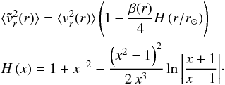 (5)For the isotropic dispersion, β(r) = 0, we can formally make the (incorrect) identification
  globally, without making any error in equating the resulting dispersions
  . In general, we can only infer
  at large radii if β is asymptotically bound (which may not hold for nearly circular orbits). This is because
  asymptotically, hence
 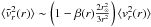 for r large enough. The relation Eq. (5) was given by Dehnen et al. (2006, Eq. (6) therein) and by Battaglia et al. (2005, the correct version can be found in the erratum Battaglia et al. 2006). For a mathematical completness we present our independent derivation of this formula in Appendix A.
While determining a PDF f = f(r,v) from the observable, a self-consistent β(r) may be looked for by iterations. The first recursion step makes the assumption  as if β(r) = 0, and a first approximation to f is obtained, from which a β(r) prediction for the next iteration step is calculated. Substituted in Eq. (5), the β(r) gives rise to a new . The process is repeated until a stable β(r) is reached. However, the distinction between and is practically unimportant unless the lower radii region is considered. In preparing the RVD profile below, we may neglect this distinction.
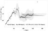 |
Fig. 1 Profile of RVD |


2.1.2. Measurements data
In our previous work (Bratek et al. 2014), we determined a RVD profile (Fig. 1), which we now assume as the basis for generating the initial conditions for the simulation in Sect. 3.1, and use it as a reference profile for comparison with the simulation results in Sect. 3.4. In preparing this profile, we assume the Sun’s distance to the Galactic centre R° = 8.5 ± 0.4 kpc, the local disk rotation speed V° = 240 ± 16 km s-1 (Bovy et al. 2009; Koposov et al. 2010) and the components of the Sun’s velocity vector with respect to the LSR (U,V,W) = (11.1 ± 1.7,12.24 ± 2.5,7.25 ± 0.9) km s-1 (Schönrich et al. 2010). We used the following position-velocity data: the halo giant stars (Dohm-Palmer et al. 2001; Starkenburg et al. 2009) from the Spaghetti Project Survey (Morrison et al. 2000); the blue horizontal branch stars (Clewley et al. 2004) from the United Kingdom Schmidt Telescope observations and SDSS; the field horizontal branch and A-type stars (Wilhelm et al. 1999) from the Beers et al. (1992) survey; the globular clusters (Harris 1996) and the dwarf galaxies (Mateo 1998). The data were recalculated to epoch J2000 when necessary. In addition, we included the ultra-faint dwarf galaxies, such as Ursa Major I and II, Coma Berenices, Canes Venatici I and II, Hercules (Simon & Geha 2007), Bootes I, Willman 1 (Martin et al. 2007), Bootes II (Koch et al. 2009), Leo V (Belokurov et al. 2008), Segue I (Geha et al. 2009), and Segue II (Belokurov et al. 2009). To eliminate a possible decrease in the RVD at lower radii due to circular orbits in the disk, we excluded tracers in the neighbourhood (R/ 20)2 + (Z/ 4)2< 1 (in units of kpc) of the mid-plane. We also did not take into account: a) a distant Leo T, located at r> 400 kpc; b) Leo I, rejected for reasons largely discussed in Bratek et al. (2014); c) a single star for which  ; and d) four additional objects for which
  (these are: 88-TARG37, Hercules, J234809.03-010737.6 and J124721.34+384157.9). As shown with the help of a simple asymptotic estimator (Bratek et al. 2014), had we not excluded d) the total expected mass would have been increased by only a factor of ≈1.16.
3. Simulation of RVD in a background field
We model the Galactic potential as consisting of: a disk-like component (accounting for the Galactic rotation curve) and a hot gaseous halo, Ψ = Ψdisk + Ψgas, of total mass Mref = 1.8 × 10¹¹ M⊙. As a starting point for further analyses, we construct an initial PDF by applying the method of Sect. 2 to the RVD profile in Fig. 1, assuming M = Mref, which is close to the lower bound for this RVD. In Fig. 2 we show the resulting PDF on the (e,ϵ) plane.
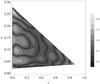 |
Fig. 2 A distribution function f(e,ϵ) consistent with the RVD profile shown in Fig. 1. The function was obtained with the help of the Keplerian ensemble method, assuming Mref = 1.8 × 10¹¹ M⊙, Rua = 18 kpc, and Rub = 240 kpc. The contour plot shows (f(e,ϵ) /fS)1 / 10, with fS being the maximum value of f(e,ϵ) on the triangular domain. |
3.1. Setting the initial conditions
The first stage towards determining the initial conditions corresponding to the PDF f(e,ϵ) shown in Fig. 2 involves generating a random set of initial radii  in the range ua<ui<ub (N is the number of all test bodies), and with the number density νu [ f ] from Eq. (2). This task can be done with the help of the inverse cumulative probability function
  of the probability density ν(u).
In the next stage, we need to ensure the spherical symmetry of the initial state. We assign to ℐ0 a set  of spherical coordinates of directions uniformly distributed on the unit sphere. This gives us the initial positions
  .
.
Next, to obtain the initial velocities, we choose random parameters (e,ϵ,ψ) consistently with the initial PDF, assigning to each (uk,θk,φk) ∈ ℐ1 an elliptic orbit; a particular test body would follow in the point mass field. To this end, we consider triples of random numbers (e,ϵ,X) uniformly distributed in their respective range: e ∈ (0,1), ϵ ∈ (0,1 / (2ua)) and X ∈ (0,fS), with X being an auxiliary variable and fS = max { f(e,ϵ):(e,ϵ) ∈ S }. For each uk ∈ ℐ0, we carry on generating random triples (e,ϵ,X) until we encounter one (labelled with a subscript k) for which both X<f(ek,ϵk) and (ek,ϵk) ∈ S(uk). This procedure yields a set of random pairs  with a non-uniform number density distribution f(e,ϵ) and each confined to a ui-dependent region S(ui). To each uk, we also assign its respective random angle ψk uniformly distributed in the range (0,2π ] and fixing the plane of the corresponding ellipse. In effect, we obtain a set
  and form the set
  . Finally, by applying the transformation Eq. (1) to each element of ℐ, we obtain the required set of initial positions and velocities in spherical coordinates, leading to an initial randomly generated RVD overlapping well with that in Fig. 1 in the region of interest.
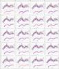 |
Fig. 3 A sequence A,B,...S,T of simulated RVD models shown at distinct simulation instants with red lines. The models were obtained from the blue line RVD (evolved from the initial PDF in the Ψdisk + Ψgas potential of total mass Mref) by rescaling the horizontal and vertical directions so as to overlap with the black line reference RVD (from measurements) as good as possible. The blue line PDF does not differ much from the violet line PDF, which assumes β = 0. The light gray region is the RVD uncertainty defined by the vertical bars in Fig. 1. The bottom figure in each panel shows a β(r) profile corresponding to its respective RVD model. The decrease in β(r) towards negative values in the lower radii region r< 40 kpc is a model artifact discussed in the text. |
3.2. Gravitational potential
The Ψdisk part of Ψ is described by the thin disk model  (6)with σ(ρ) being the column mass density of a finite-width disk found by recursions from the Galactic rotation curve in Jałocha et al. (2014). Here,
  and K is the elliptic integral of the first kind defined in Gradshtein et al. (2007). Most of the mass is enclosed within the inner disk ρ< 20 kpc: M20 = 1.49 × 10¹¹ M⊙, while M30 = 1.51 × 10¹¹ M⊙. The outer ρ> 30 kpc disk’s contribution to Eq. (6) is thus negligible and we can limit the integration to
  . To reduce the computation time, we tabulated the integral Eq. (6) at mesh points { ρj,ζk }, obtaining a smooth Ψdisk by means of the interpolating series
  with the coefficients ωpqr found by the least-squares method, minimizing the discrepancy between Eq. (6) and the series evaluated at the mesh points. Within the desired accuracy, we found this approximation procedure to be numerically more efficient than the usual two-dimensional interpolation.
Based on the OVIIKα absorption-line strengths in the spectra of galactic nuclei and galactic sources, Gupta et al. (2012) found large amounts of baryonic mass in the form of hot gas surrounding the Galaxy. Assuming a homogeneous sphere model, they found the electron density ne of 2.0 × 10⁻⁴/ cm3 and the path length L of 72 kpc. Among other parameters, the total mass of the gas depends on the gas metalicity and the oxygen-to-helium abundance. For a reasonable set of parameters, they found the total mass to be 1.2−6.1 × 10¹⁰ M⊙. We may assume Mgas = 3.0 × 10¹⁰ M⊙ consistent with these values. More recently, applying the same observational method, Miller & Bregman (2013) found the mass function M(r) of the circum-galactic hot gas using a modified density profile  We use it as the source of the spherical component Ψgas(r), with the parameters n0 = 0.46 cm-3, rc = 0.35 kpc and λ = 0.58 allowable by the best fit to the measurements. Then the integrated mass is Mgas = 3 × 10¹⁰ M⊙ at r = 100 kpc. For λ ≤ 1, the mass function is divergent and the integration must be cut off at some radius, which is to some extent arbitrary. The cutoff at 100 kpc falls within the limits 18 kpc and 200 kpc on the minimum and maximum mass of the halo considered in Miller & Bregman (2013).
3.3. Numerical solution of the equations of motion
We consider a test particle of mass m in cylindrical coordinates (ρ,ϕ,ζ), moving in an axi-symmetric gravitational field described by the potential Ψ. In this symmetry, the angular momentum component Jϕ = mρ2ϕ′(t) is conserved. On account of ϕ being a monotone function of the time t for orbits with Jϕ ≠ 0, we may regard ϕ as the independent parameter. In this parametrization, the equations of motion reduce to  (7)with
  being the angular momentum per unit mass, and vρ and vζ the velocity variables in the ortho-normal basis of the coordinate lines ρ,ζ. We solve Eq. (7) numerically by using a 4-order Runge-Kutta method with adaptive step size, controlled so as to keep below some small threshold value the relative change |Δℰ / ℰ| in the energy per unit mass
  . The relative change of energy along each trajectory during our simulation is then always smaller than 10-6: |ℰ(t) / ℰ(0) − 1| < 10-6 for all t, and this precision suffices for the purposes of this work.
3.4. Results and discussion
Using the numerical procedure of Sect. 3.3, we obtained 3665 trajectories of test bodies starting from the initial conditions of Sect. 3.1 and bound in the potential Ψdisk + Ψgas defined in Sect. 3.2. The initial state agrees with the initial PDF (Fig. 2) of a stationary solution of Jeans’ problem in the point mass potential and is consistent with the reference RVD (Fig. 1). Using these trajectories, we determined the RVD evolution from the initial one and track it through a sequence of snapshots taken at various instants, as shown in Fig. 3 (with a step size of ≈1 Gyr). Each snapshot can be regarded as an independent RVD model used to estimate the Galaxy mass by comparing the evolved RVD with the reference RVD. In this approach, the mass we assign to Ψdisk + Ψgas becomes a function of the simulation time, while the extent of that time has no physical meaning.
At this point, it is appropriate to bring attention to some features of the initial PDF that persist as model artifacts during the simulation. Namely, in the lower radii region, the evolved RVD values are reduced relative to the reference RVD. The first reason is that for the initial PDF from the point mass approximation, the velocities are too high in a fraction of objects in the modified potential, owing to a more extended mass distribution, and either quickly populate more distant regions or are not bound (in preparing the evolved RVD profiles we considered only bound trajectories). Consequently, the higher velocity values do not contribute in this region and the RVD values are reduced. The other model artifact is due to a cutoff in the PDF domain introduced in the Keplerian ensemble method to automatically prevent test bodies from penetrating the interior of a central spherical region where the point mass approximation is violated. As so, there is no limit to the number of almost nearly circular orbits that the external neighbourhood of this region can accommodate. Too many elongated orbits cannot occur there for geometrical reasons, while the admissible elongated orbits only enter this region with their pericentric sides (where radial motions are nearly vanishing). In consequence, the overall mean RVD in this neighbourhood is reduced below the observed values. Because the initial PDF has been identified with the PDF of the Keplerian ensemble, a qualitatively similar reduction mechanism in the evolved RVD comes about in the modified potential, reflecting in the β(r) reduced towards more negative values in the lower radii region. However, more circular motions in this region could be interpreted as consistent with a contribution from a cold disk. With a better initial PDF this model effect could be eliminated, but it seems of no importance for the accuracy of the total mass determination for which the region of greater radii is more important. A similar cutoff mechanism may increase the number density in the neighbourhood of the upper boundary (which we assumed to be of 240 kpc). Namely, the high RVD values observed for moderate radii, and modelled in the point mass approximation by more elongated elliptic orbits, are reduced to zero again close to the upper boundary. This reduction in the RVD appears naturally; the elongated orbits enter this region with their apocentric sides where radial motions are almost vanishing and where test bodies spent a relatively longer time, and this effect can be amplified by increasing the number density of bodies on more circular orbits. Because the model RVD is compared with the measurements at moderate radii, this effect can again be neglected.
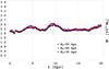 |
Fig. 4 Mass estimator μMref as a function of the simulation time, with factors μ obtained from best-fit model RVD at various threshold radii RT. |
Now, we return to the main issue. As mentioned earlier, we want to verify the expectation that the evolved PDF should be in a sense close to the initial PDF, independent of the simulation instant if the point mass approximation well describes the real situation at higher distances. If the RVD evolved in the modified potential turned out to be collapsing to much smaller values or change its shape completely, then this would mean that the mass estimate based on the initial PDF was wrong and inconsistent with the new evolved PDF.
As seen in Fig. 3, although the evolved RVD changes with the simulation time, it decreases a little in some regions and grows again later. The RVD generally remains high in the larger radii region. Similarly, the characteristic maxima in the initial RVD are not destroyed, but they oscillate. Besides the evolved RVD profile (blue line) corresponding to the mass Mref, in each snapshot we also shown a corrected RVD (red line). We consider this corrected RVD our model RVD profile, obtained by multiplying Mref and the radial variable with suitable factors close to unity, respectively μ and α, so as to make the model RVD coincide with the reference RVD as well as possible in the sense of the least squares3. During the simulation run, the length factor α varied in the range (0.85;1.02) with the mean 0.92 ± 0.03, while the mass factor μ varied in the range (1.03;1.37) with the mean 1.18 ± 0.07 (see Fig. 4). This gives the total mass estimate of (2.12 ± 0.13) × 1011 M⊙, oscillating in the range (1.85;2.47) × 1011 M⊙.
4. Conclusions
The lower bound for the Galaxy mass of ≈2.1 × 10¹¹ M⊙ obtained within the Keplerian ensemble framework is sufficient to preserve the values and qualitative features of the RVD profile from halo tracers within 150 kpc during a numerical simulation run in a modified potential. In this sense the numerically evolved RVD is stable. These results also substantiate structural stability of the point mass approximation (with more general unconstrained PDF’s), showing that the lower range for Galaxy mass estimates is reliable. A possible correction factor 1.16 to account for the four halo objects rejected in Sect. 2.1.2 would give a value of (2.5 ± 0.2) × 1011, consistent with earlier estimates of 2.4 × 10¹¹ M⊙ (Merrifield 1992; Little & Tremaine 1987) or with the value of (2.6−2.7) × 1011 M⊙ recently inferred from the kinematics of the Orphan stream (Newberg et al. 2010; Sesar et al. 2013) within ~60 kpc.
The crucial role in our analysis is played by the general unconstrained phase space. We stress that the phase-space model is not less important than the mass model, and focussing more attention on generic phase spaces might help to reduce the missing mass problem.
The dark matter halo is the most hypothetical and less constrained Galactic component. The size of the halo is usually given in terms of the virial radius defined as a radius of the sphere, which has an average density larger, by a factor of Δ = 200, than the critical density of the Universe (see e.g. McMillan 2011, because the convention for the parameter Δ is not unique). This leads to the virial mass of the halo of the order of 1012 M⊙. On the other hand, in Sect. 1 we argued that the dark matter halo with a low mass of about the lower bound M ≈ 2 × 10¹¹ M⊙ and the size of about r ≈ 20 kpc is also allowed by the RVD profile observations, whereas, as we mentioned in Sect. 1, in the literature the mass estimates based on the RVD profile Galaxy differ from each other by a factor larger than two. This shows that the total mass of the halo is poorly constrained by the motions of the distant tracers.
We present here an extreme example of a model without NDM halo, and we have shown the model to be stable in a sense that it accounts for the measured RVD at each simulation instant. This shows that our model can be thought of as a collisionless system close to a steady state. The possibility of accounting for the RVD observations without NDM halo shows that either the halo is unnecessary for the understanding of the motions of the kinematical tracers, or that other observational features (e.g. the measurements of the β(r) function) are needed to define constraints on the phase space, which would allow to disambiguate between various halo mass profiles.
This paragraph summarizes the mathematical basis of our method discussed in more detail in Bratek et al. (2014).
In place of (e,ϵ,u) it is more convenient to use coordinates (α,β,u), such that  ,
,  . A motivation behind this mapping and its explicit construction is given in Bratek et al. (2014).
References
- Bahcall, J. N., & Tremaine, S. 1981, ApJ, 244, 805 [NASA ADS] [CrossRef] [Google Scholar]
- Battaglia, G., Helmi, A., Morrison, H., et al. 2005, MNRAS, 364, 433 [NASA ADS] [CrossRef] [Google Scholar]
- Battaglia, G., Helmi, A., Morrison, H., et al. 2006, MNRAS, 370, 1055 [NASA ADS] [CrossRef] [Google Scholar]
- Beers, T. C., Preston, G. W., & Shectman, S. A. 1992, AJ, 103, 1987 [NASA ADS] [CrossRef] [Google Scholar]
- Belokurov, V., Walker, M. G., Evans, N. W., et al. 2008, ApJ, 686, L83 [NASA ADS] [CrossRef] [Google Scholar]
- Belokurov, V., Walker, M. G., Evans, N. W., et al. 2009, MNRAS, 397, 1748 [NASA ADS] [CrossRef] [Google Scholar]
- Bovy, J., Hogg, D. W., & Rix, H.-W. 2009, ApJ, 704, 1704 [NASA ADS] [CrossRef] [Google Scholar]
- Bratek, Ł., Sikora, S., Jałocha, J., & Kutschera, M. 2014, A&A, 562, A134 [NASA ADS] [CrossRef] [EDP Sciences] [Google Scholar]
- Clewley, L., Warren, S. J., Hewett, P. C., Norris, J. E., & Evans, N. W. 2004, MNRAS, 352, 285 [NASA ADS] [CrossRef] [Google Scholar]
- Deason, A. J., Belokurov, V., Evans, N. W., & An, J. 2012a, MNRAS, 424, L44 [NASA ADS] [CrossRef] [Google Scholar]
- Deason, A. J., Belokurov, V., Evans, N. W., et al. 2012b, MNRAS, 425, 2840 [NASA ADS] [CrossRef] [Google Scholar]
- Dehnen, W., McLaughlin, D. E., & Sachania, J. 2006, MNRAS, 369, 1688 [NASA ADS] [CrossRef] [Google Scholar]
- Dohm-Palmer, R. C., Helmi, A., Morrison, H., et al. 2001, ApJ, 555, L37 [NASA ADS] [CrossRef] [Google Scholar]
- Geha, M., Willman, B., Simon, J. D., et al. 2009, ApJ, 692, 1464 [NASA ADS] [CrossRef] [Google Scholar]
- Gradshtein, I., Ryzhik, I., Jeffrey, A., & Zwillinger, D. 2007, Table of integrals, series and products, Academic Press (Academic Press) [Google Scholar]
- Gupta, A., Mathur, S., Krongold, Y., Nicastro, F., & Galeazzi, M. 2012, ApJ, 756, L8 [NASA ADS] [CrossRef] [Google Scholar]
- Harris, W. E. 1996, AJ, 112, 1487 [NASA ADS] [CrossRef] [Google Scholar]
- Jałocha, J., Sikora, S., Bratek, Ł., & Kutschera, M. 2014, A&A, 566, A87 [NASA ADS] [CrossRef] [EDP Sciences] [Google Scholar]
- Jeans, J. H. 1915, MNRAS, 76, 70 [NASA ADS] [CrossRef] [Google Scholar]
- Kafle, P. R., Sharma, S., Lewis, G. F., & Bland-Hawthorn, J. 2014, ApJ, 794, 59 [NASA ADS] [CrossRef] [Google Scholar]
- Klypin, A., Zhao, H., & Somerville, R. S. 2002, ApJ, 573, 597 [Google Scholar]
- Koch, A., Wilkinson, M. I., Kleyna, J. T., et al. 2009, ApJ, 690, 453 [NASA ADS] [CrossRef] [Google Scholar]
- Kochanek, C. S. 1996, ApJ, 457, 228 [NASA ADS] [CrossRef] [Google Scholar]
- Koposov, S. E., Rix, H.-W., & Hogg, D. W. 2010, ApJ, 712, 260 [NASA ADS] [CrossRef] [Google Scholar]
- Little, B., & Tremaine, S. 1987, ApJ, 320, 493 [NASA ADS] [CrossRef] [Google Scholar]
- Magorrian, J. 2014, MNRAS, 437, 2230 [NASA ADS] [CrossRef] [Google Scholar]
- Martin, N. F., Ibata, R. A., Chapman, S. C., Irwin, M., & Lewis, G. F. 2007, MNRAS, 380, 281 [NASA ADS] [CrossRef] [Google Scholar]
- Mateo, M. L. 1998, ARA&A, 36, 435 [NASA ADS] [CrossRef] [Google Scholar]
- McMillan, P. J. 2011, MNRAS, 414, 2446 [NASA ADS] [CrossRef] [Google Scholar]
- Merrifield, M. R. 1992, AJ, 103, 1552 [NASA ADS] [CrossRef] [Google Scholar]
- Miller, M. J., & Bregman, J. N. 2013, ApJ, 770, 118 [NASA ADS] [CrossRef] [Google Scholar]
- Morrison, H. L., Mateo, M., Olszewski, E. W., et al. 2000, AJ, 119, 2254 [NASA ADS] [CrossRef] [Google Scholar]
- Navarro, J. F., Frenk, C. S., & White, S. D. M. 1997, ApJ, 490, 493 [NASA ADS] [CrossRef] [Google Scholar]
- Newberg, H. J., Willett, B. A., Yanny, B., & Xu, Y. 2010, ApJ, 711, 32 [NASA ADS] [CrossRef] [Google Scholar]
- Sakamoto, T., Chiba, M., & Beers, T. C. 2003, A&A, 397, 899 [NASA ADS] [CrossRef] [EDP Sciences] [Google Scholar]
- Schönrich, R., Binney, J., & Dehnen, W. 2010, MNRAS, 403, 1829 [NASA ADS] [CrossRef] [Google Scholar]
- Sesar, B., Grillmair, C. J., Cohen, J. G., et al. 2013, ApJ, 776, 26 [NASA ADS] [CrossRef] [Google Scholar]
- Sikora, S., Bratek, Ł., Jałocha, J., & Kutschera, M. 2012, A&A, 546, A126 [NASA ADS] [CrossRef] [EDP Sciences] [Google Scholar]
- Simon, J. D., & Geha, M. 2007, ApJ, 670, 313 [NASA ADS] [CrossRef] [Google Scholar]
- Starkenburg, E., Helmi, A., Morrison, H. L., et al. 2009, ApJ, 698, 567 [NASA ADS] [CrossRef] [Google Scholar]
- Watkins, L. L., Evans, N. W., & An, J. H. 2010, MNRAS, 406, 264 [NASA ADS] [CrossRef] [Google Scholar]
- Wilhelm, R., Beers, T. C., Sommer-Larsen, J., et al. 1999, AJ, 117, 2329 [NASA ADS] [CrossRef] [Google Scholar]
- Wilkinson, M. I., & Evans, N. W. 1999, MNRAS, 310, 645 [NASA ADS] [CrossRef] [Google Scholar]
- Xue, X. X., Rix, H. W., Zhao, G., et al. 2008, ApJ, 684, 1143 [NASA ADS] [CrossRef] [Google Scholar]
Appendix A: Derivation of a relation between the observable  and the radial dispersion
Let v be the Galacto-centric velocity vector. Expressed in terms of its radial Vr and transversal components Vθ,Vφ it reads  Vθcosθ)sinφ + Vφcosφ,Vrcosθ − Vθsinθ]. As er =
 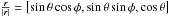 and r⊙ = [r⊙,0,0] the l.o.s versor is
 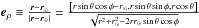 . We take the mean values
  and
and  over thin spherical shells and consider them as functions of the Galacto-centric distance r. For a spherically symmetric system, we define as
 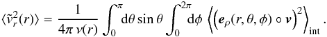 Here, ⟨ ·⟩ int is the averaging over the velocities weighted by a spherically symmetric PDF f(r,v(r)), normalized so as ν(r) ⟨ (·) ⟩ int ≡ ∫(·)f(r,v(r)) d3v, with ν denoting the number density. The scalar product squared
  is a homogenuous form of second degree in the velocities Vr,Vθ,Vφ with coefficients being functions of r,θ,φ. With a direct inspection, one can notice that the integration over θ,φ of the coefficients standing at VrVθ, VθVφ, VφVr, gives zero (the velocity products are independent of θ,φ). Thus, upon integration over the velocities, we can focus only on the terms involving dispersions
  ,
,  ,
,  . Furthermore, it also follows from the spherical symmetry that
  and, trivially, that the ratios
  ,
,  define the same function of r. In accordance with the common convention in the theory of spherical Jeans equations, we express this function in terms of the flattening of the dispersion ellipsoid, β(r). Then, by making the substitution
  and
and  , we obtain that
 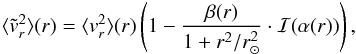 where
where  for r ≠ r⊙ and
 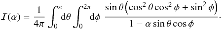 We recall that all integrals that are zero by symmetries have already been omitted in the expression for ℐ(α). Because the requirements for the integration of a functional series term by term and its limit are met for 0 ≤ α< 1, the integral ℐ(α) can be calculated by a Taylor series expansion in α (note that owing to the vanishing of the integrals
  with odd m, only even powers of α are present in the series). On reducing the summands with the help of the Pythagorean trigonometric identity, the remaining non-zero coefficients in the power series in α arrange to products of elementary definite integrals
  , where
  ;
;  . Now,
  and
and  . Hence,
  , where we have subtracted the excess term 2α in the second series after renaming n → n + 1. Both of the infinite series are Taylor series expansions of
  , therefore,
 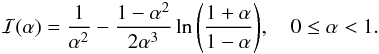 Next, using the earlier expression for
  and substituting the definition of α(r) in place of α, we finally obtain Eq. (5).
All Figures
|
Fig. 1 Profile of RVD |
| In the text | |
|
Fig. 2 A distribution function f(e,ϵ) consistent with the RVD profile shown in Fig. 1. The function was obtained with the help of the Keplerian ensemble method, assuming Mref = 1.8 × 10¹¹ M⊙, Rua = 18 kpc, and Rub = 240 kpc. The contour plot shows (f(e,ϵ) /fS)1 / 10, with fS being the maximum value of f(e,ϵ) on the triangular domain. |
| In the text | |
|
Fig. 3 A sequence A,B,...S,T of simulated RVD models shown at distinct simulation instants with red lines. The models were obtained from the blue line RVD (evolved from the initial PDF in the Ψdisk + Ψgas potential of total mass Mref) by rescaling the horizontal and vertical directions so as to overlap with the black line reference RVD (from measurements) as good as possible. The blue line PDF does not differ much from the violet line PDF, which assumes β = 0. The light gray region is the RVD uncertainty defined by the vertical bars in Fig. 1. The bottom figure in each panel shows a β(r) profile corresponding to its respective RVD model. The decrease in β(r) towards negative values in the lower radii region r< 40 kpc is a model artifact discussed in the text. |
| In the text | |
|
Fig. 4 Mass estimator μMref as a function of the simulation time, with factors μ obtained from best-fit model RVD at various threshold radii RT. |
| In the text | |
Current usage metrics show cumulative count of Article Views (full-text article views including HTML views, PDF and ePub downloads, according to the available data) and Abstracts Views on Vision4Press platform.
Data correspond to usage on the plateform after 2015. The current usage metrics is available 48-96 hours after online publication and is updated daily on week days.
Initial download of the metrics may take a while.