| Issue |
A&A
Volume 579, July 2015
|
|
|---|---|---|
| Article Number | A16 | |
| Number of page(s) | 6 | |
| Section | The Sun | |
| DOI | https://doi.org/10.1051/0004-6361/201525716 | |
| Published online | 19 June 2015 | |
Fast approximate radiative transfer method for visualizing the fine structure of prominences in the hydrogen Hα line
1
Astronomical Institute, The Czech Academy of Sciences,
Czech Republic, 25165
Ondřejov, Czech
Republic
e-mail: This email address is being protected from spambots. You need JavaScript enabled to view it.
2
School of Mathematics and Statistics, University of St
Andrews, North
Haugh, St Andrews,
KY16 9SS,
UK
3
Max-Planck-Institut für Astrophysik, Karl-Schwarzschild-Str. 1, 85740
Garching bei München,
Germany
Received: 22 January 2015
Accepted: 9 April 2015
Abstract
Aims. We present a novel approximate radiative transfer method developed to visualize 3D whole-prominence models with multiple fine structures using the hydrogen Hα spectral line.
Methods. This method employs a fast line-of-sight synthesis of the Hα line profiles through the whole 3D prominence volume and realistically reflects the basic properties of the Hα line formation in the cool and low-density prominence medium. The method can be applied both to prominences seen above the limb and filaments seen against the disk.
Results. We provide recipes for the use of this method for visualizing the prominence or filament models that have multiple fine structures. We also perform tests of the method that demonstrate its accuracy under prominence conditions.
Conclusions. We demonstrate that this fast approximate radiative transfer method provides realistic synthetic Hα intensities useful for a reliable visualization of prominences and filaments. Such synthetic high-resolution images of modeled prominences/filaments can be used for a direct comparison with high-resolution observations.
Key words: radiative transfer / Sun: filaments, prominences / Sun: magnetic fields
On leave from Astronomical Institute of the Czech Academy of Sciences.
© ESO, 2015
1. Introduction
During the past two decades, a significant effort was devoted to 3D modeling of prominence magnetic structures – see, for example, the reviews by Mackay et al. (2010), van Ballegooijen & Su (2014), and Gunár (2014). For quiescent prominences, a variety of magnetic field configurations with numerous magnetic dips was produced with these models. These magnetic dips are routinely visualized schematically by plotting their characteristic length, often corresponding to one pressure scale-height (300 km if assuming an isothermal plasma with a temperature of 10 000 K), see, for instance, Aulanier & Démoulin (1998), Dudík et al. (2008), Mackay & van Ballegooijen (2009), and Su & van Ballegooijen (2012). Such illustrative visualization provides an idea about the global pattern of the prominence or filament structures. However, the magnetic field configurations visualized in this way cannot be directly compared with high-resolution images of the prominence or filament fine structures obtained by various instruments, often in the Hα line. The main reason is that the prominence Hα visibility largely depends on the number of fine structures projected into the line of sight (LOS). And while the Hα optical thickness of individual prominence fine structures may be significantly below unity, the total optical thickness along the LOS in typical quiescent prominences is larger. The effects of radiative transfer along the LOS therefore have to be taken into account to provide more realistic prominence visualizations.
To visualize a prominence consisting of many dips, first individual magnetic dips must be filled by the plasma with realistic temperature and gas pressure distributions and then, ideally, one has to perform 3D radiative-transfer modeling of such highly heterogeneous prominence to predict its visibility in a given spectral line. One way to fill the dips with prominence plasma is to consider the thermal non-equilibrium models of Karpen et al. (2006), which are based on the heating and evaporation of the chromospheric plasma and its subsequent cooling and condensation inside the magnetic dips. Luna et al. (2012) have shown that these prominence formation models can predict the signatures of hotter parts of the prominence fine structures (such as thermal properties, velocities, and mass loading) but do not directly provide the Hα visibility of the cool fine structures. Recently, Gunár et al. (2013) developed a method allowing to fill individual force-free magnetic dips with the prominence plasma in a hydrostatic equilibrium. These dips can be approximated by 2D vertically infinite threads similar to those of Heinzel & Anzer (2001), and thus the 2D non-LTE (i.e., departures from local thermodynamic equilibrium) radiative transfer modeling can be used to obtain their radiative output in hydrogen spectral lines. Gunár & Mackay (2015) used the method of filling the force-free dips with prominence plasma to construct the first 3D whole-prominence fine structure (WPFS) models. These are based on the nonlinear force-free field simulations of the entire prominence magnetic field (Mackay & van Ballegooijen 2009) and contain realistic prominence plasma distributed along a large number of fine structures. However, an implementation of the full 3D non-LTE computations to such extensive highly heterogeneous models with hundreds of prominence fine structures would present a task that is extremely demanding on computing resources. This is dictated by the need to use fine grid-spacing down to a few km to properly resolve steep temperature gradients within individual plasma fine structures. Such fine grid-spacing is also required to accurately solve the radiative transfer in the optically thick lines such as the Lyman-α line of hydrogen. Moreover, the structure of entire prominences can span large dimensions on the order of 200 000 × 50 000 × 20 000 km (Gunár & Mackay 2015). This would lead to extremely large computational grids, and even with adaptive mesh refinement such computations would still significantly exceed the computing requirements of current massive radiation-magneto-hydrodynamic simulations such as the 3D chromospheric simulations of Leenaarts et al. (2012) and Leenaarts et al. (2015).
In this paper we present a fast approximate method for visualizing 3D whole-prominence models in the Hα line that can be used for imaging of the cool prominence structures. This method is based on our experience with the Hα line formation in prominences, see, for example, Heinzel (2015). It employs a fast line-of-sight synthesis of the Hα line profiles through the whole 3D prominence volume and realistically reflects the basic properties of the Hα line formation in the cool and low-density prominence medium. The method can be applied both to prominences seen above the limb and to filaments seen against the disk. It was recently used by Gunár & Mackay (2015) to visualize their 3D WPFS model.
We present the Hα visualization method in Sect. 2 and give recipes for its use in Sect. 3. Section 3 also provides the results of several tests comparing 1D and 2D non-LTE radiative transfer models and the new fast visualization method. In Sect. 4 we present a sample image of visualized force-free magnetic dips, and in Sect. 5 we discuss our results and make conclusions.
2. Hα synthesis
The Hα
intensity is obtained by the LOS integration of the radiative transfer equation through
generally nonuniform prominence media. To obtain the Hα intensity, we must know the
distribution of the line source function and the opacity along the LOS. The specific
intensity is then obtained from the formal solution of the radiative transfer equation
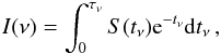 (1)where
 (2)The term dtν represents the
optical-depth increment corresponding to the geometrical path increment dl, and κ(ν,l) is
the absorption coefficient for the Hα line. τν is the total optical
thickness integrated through all structures crossed by a given LOS. Assuming a uniform
source function in the whole medium, Eq. (1)
reduces to the well-known from (see, e.g., Heinzel
2015)
(2)The term dtν represents the
optical-depth increment corresponding to the geometrical path increment dl, and κ(ν,l) is
the absorption coefficient for the Hα line. τν is the total optical
thickness integrated through all structures crossed by a given LOS. Assuming a uniform
source function in the whole medium, Eq. (1)
reduces to the well-known from (see, e.g., Heinzel
2015)  (3)The absorption coefficient for the
Hα line has
the standard form
(3)The absorption coefficient for the
Hα line has
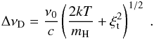
the standard form 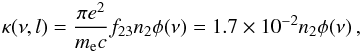 (4)where f23 is the
Hα line
oscillator strength, n2 is the hydrogen second-level
population, and φ(ν) is the normalized absorption
profile. Since the individual fine structures are assumed to be optically thin (see below),
the absorption line profile is well approximated by a Gaussian profile in our case,
depending on the thermal and microturbulent broadening
(4)where f23 is the
Hα line
oscillator strength, n2 is the hydrogen second-level
population, and φ(ν) is the normalized absorption
profile. Since the individual fine structures are assumed to be optically thin (see below),
the absorption line profile is well approximated by a Gaussian profile in our case,
depending on the thermal and microturbulent broadening
 (5)where
 (6)We assume a given LOS distribution of the
kinetic temperature T and gas pressure pg. The
microturbulent velocity is difficult to determine and thus we take a representative value of
5 km s-1 in the whole
prominence (see, e.g., Engvold et al. 1990; Labrosse et al. 2010). Certain variations would not
affect the Hα
prominence visibility significantly. To compute the line intensity according to Eq. (1), we need to know the value of the source
function and the LOS variations of the hydrogen second-level population, which enters the
absorption coefficient, see Eq. (4).
(6)We assume a given LOS distribution of the
kinetic temperature T and gas pressure pg. The
microturbulent velocity is difficult to determine and thus we take a representative value of
5 km s-1 in the whole
prominence (see, e.g., Engvold et al. 1990; Labrosse et al. 2010). Certain variations would not
affect the Hα
prominence visibility significantly. To compute the line intensity according to Eq. (1), we need to know the value of the source
function and the LOS variations of the hydrogen second-level population, which enters the
absorption coefficient, see Eq. (4).
2.1. Hα line source function
Under typical prominence conditions, the Hα line source function is dominated by the
scattering of the incident radiation from the solar disk (Heinzel 2015), which depends on the altitude of the prominence material above
the solar surface. For an altitude of 10 000 km, Gouttebroze et al. (1993) constructed a grid of 140 isothermal-isobaric 1D slab
models and tabulated various structural and radiative quantities. Based on this, Heinzel et al. (1994) demonstrated several important
correlations between these quantities. One of the most important results is that the
Hα source
function is nearly constant in 1D slabs for the line-center optical thicknesses up to
unity. Above this value, the Hα source function starts to increase (see Fig. 18
in Heinzel et al. 1994). At an altitude of 10 000
km the source function S is fixed at a value approximately equal to the
diluted Hα
line-center intensity at the solar disk center, which is W × 0.17 × 4.077 ×
10-5 erg s-1 cm-2 sr-1 Hz-1. The dilution factor W has the form
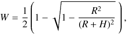 (7)where H represents the height
above the solar surface and R is the solar radius (see, e.g., the Appendix in
Jejčič & Heinzel 2009). The factor 0.17
corresponds to the central depression of the Hα line at the disk center (David 1961) and 4.077 ×
10-5 erg s-1 cm-2 sr-1 Hz-1 is the disk-center continuum intensity near the
Hα line.
(7)where H represents the height
above the solar surface and R is the solar radius (see, e.g., the Appendix in
Jejčič & Heinzel 2009). The factor 0.17
corresponds to the central depression of the Hα line at the disk center (David 1961) and 4.077 ×
10-5 erg s-1 cm-2 sr-1 Hz-1 is the disk-center continuum intensity near the
Hα line.
The prominence fine structures are typically small and numerous along a given LOS. While the total Hα optical thickness of large prominences may reach values higher than one, we therefore assume that each fine structure element (magnetic dip filled with the prominence plasma) is optically thin in Hα. This allows us to use a uniform value of the line source function at the given altitude. For different altitudes this value scales roughly with the ratio of the dilution factors (see Sect. 2.3). Note also that the Hα line source function is frequency-independent in the CRD (complete frequency redistribution) approximation. Specifying the Hα line source function in this way, we assumed that all structures are independently illuminated by the solar disk radiation and that they do not interact radiatively among themselves. However, the Hα source function will remain similar even for more densely packed structures.
2.2. Hα absorption coefficient
The only unknown quantity in Eq. (4) is
the population (number density) of hydrogen atoms in the second quantum level
n2. To determine this in an approximate
way, we use the relation between the electron density and the hydrogen second-level
population 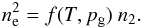 (8)This relation was derived by various authors,
and its nature is explained in Heinzel et al.
(1994), who found f ≃
3 × 1016 cm-3 for T = 8000 K. The same value was also reported by
Landman & Mongillo (1979). In general, this
factor mildly depends on the temperature and gas pressure (see Table 1). The electron density can be estimated from the
local values of the gas pressure and the temperature using the following set of formulas:
(8)This relation was derived by various authors,
and its nature is explained in Heinzel et al.
(1994), who found f ≃
3 × 1016 cm-3 for T = 8000 K. The same value was also reported by
Landman & Mongillo (1979). In general, this
factor mildly depends on the temperature and gas pressure (see Table 1). The electron density can be estimated from the
local values of the gas pressure and the temperature using the following set of formulas:
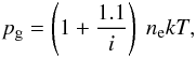
 (9)where N is the total particle
number density given by N =
nH + nHe +
ne. Here, nH is the total
hydrogen density – the sum of the neutral hydrogen and the proton density, and
nHe is the helium density. Assuming 10%
abundance of the helium and no helium ionization (fully ionized helium would contribute to
the electron density by 20%), we can write
(9)where N is the total particle
number density given by N =
nH + nHe +
ne. Here, nH is the total
hydrogen density – the sum of the neutral hydrogen and the proton density, and
nHe is the helium density. Assuming 10%
abundance of the helium and no helium ionization (fully ionized helium would contribute to
the electron density by 20%), we can write
 (10)where i =
ne/nH is the
hydrogen ionization degree. The value of i depends on temperature and gas pressure and is
specified below.
(10)where i =
ne/nH is the
hydrogen ionization degree. The value of i depends on temperature and gas pressure and is
specified below.
2.3. Parameters S, f, and i
Values of the ionization degree i and the parameter f for various values of the temperature (in K) and gas pressure (in dyn cm-2).
Mean values of i and f can be inferred from the correlation plots of Heinzel et al. (1994). However, for this new Hα visualization method we evaluated these parameters for a broader range of temperatures using the most advanced 1D non-LTE radiative transfer models recently implemented by Heinzel et al. (2014). The results are given in Table 1 for three representative altitudes of 10 000, 20 000, and 30 000 km and for a nominal slab thickness of 500 km. For the isothermal-isobaric slabs of Heinzel et al. (2014) that are not optically thick in Hα, the atomic level populations and the electron densities are almost constant inside the slabs (Gouttebroze et al. 1993), and we took the values at the slab center to tabulate i and f. For the same altitudes we also determined average values of the Hα line source function S as 3.22 × 10⁻⁶, 2.98 × 10⁻⁶, and 2.80 × 10⁻⁶ erg s-1 cm-2 sr-1 Hz-1, respectively. The values of S and f can be approximately scaled in altitude by the ratio of the dilution factors, as these quantities are proportional to the dilution factor by their very nature. The ionization degree i varies much less with the altitude and is not directly related to the dilution factor W.
3. Recipes for prominence or filament visualizations
To visualize the whole-prominence magnetic field configuration containing many magnetic
dips filled with the plasma having a given temperature and pressure distribution, we proceed
in the following way. First, we compute the LOS optical thickness
 (11)where the line absorption coefficient
κ(ν,l) is given by Eq. (4). For a given height above the solar surface,
we can interpolate the value of the Hα source function given in Sect. 2.3. The values of i and f entering the evaluation of the absorption
coefficient are obtained from Table 1 for the local
values of T and
pg
along the LOS. Then Eq. (3) is used to
compute the synthetic line profile for each LOS (a pixel in the simulated image). To obtain
the synthetic image for a specific Hα filter, one has to multiply the emission line
profile by the filter response function and integrate over the wavelength range of the
filter sensitivity. We note that for τν> 1, the line
intensity will saturate to the value of the source function, as evident from Eq. (3).
(11)where the line absorption coefficient
κ(ν,l) is given by Eq. (4). For a given height above the solar surface,
we can interpolate the value of the Hα source function given in Sect. 2.3. The values of i and f entering the evaluation of the absorption
coefficient are obtained from Table 1 for the local
values of T and
pg
along the LOS. Then Eq. (3) is used to
compute the synthetic line profile for each LOS (a pixel in the simulated image). To obtain
the synthetic image for a specific Hα filter, one has to multiply the emission line
profile by the filter response function and integrate over the wavelength range of the
filter sensitivity. We note that for τν> 1, the line
intensity will saturate to the value of the source function, as evident from Eq. (3).
The same procedure can be also applied to visualize filaments viewed against the solar
disk. However, in this case, the background disk radiation attenuated by the filament must
be added, that is,  (12)Depending on the position of the filament on
the solar disk, the background Hα intensity Ibgr can be
obtained from David (1961), for instance, and using
the limb-darkened continuum intensity in the vicinity of the Hα line (Allen 1976). We note that for filaments, S varies with height along
the LOS (see Sect. 2.3), which might require a more
accurate solution.
(12)Depending on the position of the filament on
the solar disk, the background Hα intensity Ibgr can be
obtained from David (1961), for instance, and using
the limb-darkened continuum intensity in the vicinity of the Hα line (Allen 1976). We note that for filaments, S varies with height along
the LOS (see Sect. 2.3), which might require a more
accurate solution.
The visualization method presented here can also accommodate LOS velocities on the order of
10 km s-1. Such
velocities are typically encountered in quiescent prominences, see Gunár et al. (2012), for example. The source function and the ionization
degree are not significantly affected by such velocities, which allows us to use the same
tabulated values of S, f, and i. These velocities therefore only affect the
absorption coefficient κ(ν,l). Taking into account a local
Doppler shift Δν′(l) due to the local LOS
velocity, we can modify Eq. (4) as
 (13)
(13)
3.1. Tests of the method
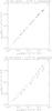 |
Fig. 1 Scatterplots of the Hα line center intensities obtained by 1D non-LTE computations (x-axes) and by approximate synthesis using i and f interpolation (top) and using fixed representative i and f values (bottom). Dashed lines correspond to the precise match with the intensities obtained by 1D non-LTE computations. |
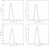 |
Fig. 2 Optical thickness (left column) and intensity (right column) at the Hα line center plotted along the length of the 2D plasma structure of the Deep_dip (upper row) and the Model_dem (lower row). Solid lines represent the 2D non-LTE radiative transfer calculations, while the dash-dotted lines show the results of the approximate Hα synthesis with the interpolation of i and f. |
To demonstrate the accuracy of our Hα visualization method, we performed several tests comparing the Hα line intensities obtained by 1D and 2D non-LTE radiative transfer models with the results of the fast approximate Hα synthesis.
In the first test we used the series of 1D non-LTE isothermal-isobaric models of Heinzel et al. (2014). We compared the Hα line-center intensities obtained by the models with the intensities computed by the Hα synthesis when using the interpolation of parameters i and f from the tables provided in this paper and when using representative fixed values of parameters i and f for all models. All results are valid for the altitude of 10 000 km. In Fig. 1 (top) we show the scatterplot of the Hα line-center intensities obtained by 1D non-LTE computations (x-axis) and our approximate synthesis using i and f interpolation (y-axis). The bottom part of Fig. 1 shows the same scatterplot, but using the approximate synthesis with representative values of i = 0.35 and f = 4.7 × 1016 cm-3. It is evident that the intensities obtained by the approximate synthesis with i and f interpolation agree very well with the intensities obtained by exact 1D non-LTE computations. The approximate synthesis with selected representative i and f values also produces results that agree reasonably well with the exact solutions.
In the second test we used the 2D temperature and gas pressure distribution inside the force-free magnetic dip named Deep_dip presented in Gunár et al. (2013), see Fig. 6 therein. We scanned its 2D structure along its length with the LOS perpendicular to the x-axis and at each position computed the Hα line-center intensity and optical thickness using the approximate Hα synthesis with the interpolation of i and f. We compared this with the results of the 2D non-LTE radiative transfer modeling reported by Gunár et al. (2013). In the top row of Fig. 2 we plot the optical thickness (left) and the intensity (right) at the Hα line center along the length of the magnetic dip. Solid lines represent the full 2D non-LTE radiative transfer calculations and dashed-dotted lines show the approximate Hα synthesis. In the bottom row of Fig. 2 we show the same, but for the 2D fine-structure thread model Model_dem presented by Gunár et al. (2011), see Fig. 6 therein. Again, we plot the optical thickness (left) and the intensity (right) using solid lines for the full 2D non-LTE radiative transfer calculations and dashed-dotted lines for the approximate Hα synthesis. The plots in Fig. 2 show that the approximate synthesis is also able to reproduce the optical thickness and the intensity of the Hα line center as derived by more complex 2D non-LTE calculations reasonably well. This represents an important confirmation of the reliability of the approximate synthesis method that is based on the 1D prominence fine-structure modeling (Heinzel et al. 2014). A mild influence of the 2D radiative transfer effects is apparent in the first row of Fig. 2, where the discrepancy at the sides of the structure (wings of the plotted τ and I profiles) can be attributed to the influence of the incident radiation penetrating the 2D structure from the sides. The approximate 1D synthesis cannot account for these boundary effects. The discrepancy between the approximate 1D synthesis and the 2D non-LTE calculations shown in the second row of Fig. 2 might also be caused by the 2D radiative transfer effects. In this case, the approximate synthesis underestimates the Hα line center optical thickness and intensity in the middle of the structure while correctly representing its sides. We note that our test-cases represent different 2D prominence fine-structure models – the first based on the force-free magnetic dips and the second using gravity-induced dips. We used them to demonstrate the ability of the approximate Hα synthesis method to reproduce results for a wide variety of models, but it is not our aim to compare these models with each other.
4. Sample image of the prominence magnetic dip
To illustrate the application of the approximate Hα line synthesis method presented here, we visualized two force-free magnetic dips filled with prominence plasma. The magnetic field configuration of these dips was obtained by the 3D nonlinear force-free field simulations of the whole prominence magnetic structure by Mackay & van Ballegooijen (2009). These dips were filled with prominence plasma in the hydrostatic equilibrium according to the method of Gunár et al. (2013). One of the visualized dips is the Deep_dip, representing a prominence fine structure with higher gas pressure in its center due to its significant depth, see Gunár et al. (2013). The other dip is shallower (but not the Shallow_dip of Gunár et al. 2013), resulting in a much lower central gas pressure. It is also more extended along the magnetic field, about 65 000 km compared to the 50 000 km of the Deep_dip. Both dips simulate prominence fine structures with an assumed cross-section of 1000 km. In Fig. 3 we show a synthetic image in the Hα line center where the Deep_dip is placed above the shallower dip. The Deep_dip appears much brighter due to its higher central gas pressure. Moreover, it also appears somewhat longer than the (in reality more extended) shallower dip. This can be attributed to the Hα visibility of the prominence material.
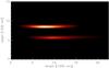 |
Fig. 3 Synthetic image in the Hα line center of the Deep_dip (upper structure) and a shallower dip (lower structure). |
5. Discussion and conclusions
As mentioned above, our approximate Hα visualization method assumes that the individual fine-structure elements do not interact radiatively, and thus each of them is only illuminated by the incident solar radiation. In this case, their Hα line source function can be determined using the non-LTE radiative transfer model (1D slabs in our case) for individual fine structures. For these 1D models we considered rather narrow slabs of 500 km thickness to obtain the values of S, i, and f tabulated in Sect. 2.3. These values are taken at the slab center but result from the radiative transfer within the whole slab. However, in the approximate Hα synthesis method we considered them as local values. This assumption introduces certain errors in the estimates of the true local values of these parameters. However, the tests presented in Sect. 3.1 show that our approximate Hα visualization method is sufficiently accurate. We note that this accuracy would break down in an extreme case when all prominence fine structures were densely packed close to each other within a large prominence. This scenario may be simulated by a large homogeneous slab that is only illuminated at its two boundaries. In this case, the depth-dependent behavior of the source function will be different, reflecting the actual conditions within the (optically thick) slab – see Gouttebroze et al. (1993).
We have demonstrated that our fast approximate radiative transfer method for vizualising the Hα prominence provides realistic synthetic Hα intensities that are useful for a reliable visualization of prominences and filaments. Such synthetic high-resolution images of whole prominences/filaments are quantitatively accurate enough and thus can be used for a direct comparison with radiometrically calibrated observations.
Acknowledgments
P.H. acknowledges the support from grant 209/12/0906 of the Grant Agency of the Czech Republic. S.G. acknowledges support from the European Commission via the Marie Curie Actions – Intra-European Fellowships Project No. 328138. P.H. and S.G. acknowledge support from project RVO:67985815 of the Astronomical Institute of the Czech Academy of Sciences and from the MPA Garching. U.A. thanks for the support from the Astronomical Institute of the Czech Academy of Sciences.
References
- Allen, C. W. 1976, Astrophysical Quantities (London: The Athlone Press) [Google Scholar]
- Aulanier, G., & Démoulin, P. 1998, A&A, 329, 1125 [Google Scholar]
- David, K.-H. 1961, Z. Astrophys., 53, 37 [NASA ADS] [Google Scholar]
- Dudík, J., Aulanier, G., Schmieder, B., Bommier, V., & Roudier, T. 2008, Sol. Phys., 248, 29 [NASA ADS] [CrossRef] [Google Scholar]
- Engvold, O., Hirayama, T., Leroy, J. L., Priest, E. R., & Tandberg-Hanssen, E. 1990, in Dynamics of Quiescent Prominences, eds. V. Ruzdjak & E. Tandberg-Hanssen (New York: Springer Verlag), IAU Colloq., 363, 294 [Google Scholar]
- Gouttebroze, P., Heinzel, P., & Vial, J. C. 1993, A&AS, 99, 513 [NASA ADS] [Google Scholar]
- Gunár, S. 2014, in IAU Symp. 300, eds. B. Schmieder, J.-M. Malherbe, & S. T. Wu, 59 [Google Scholar]
- Gunár, S., & Mackay, D. H. 2015, ApJ, 803, 64 [NASA ADS] [CrossRef] [Google Scholar]
- Gunár, S., Parenti, S., Anzer, U., Heinzel, P., & Vial, J.-C. 2011, A&A, 535, A122 [NASA ADS] [CrossRef] [EDP Sciences] [Google Scholar]
- Gunár, S., Mein, P., Schmieder, B., Heinzel, P., & Mein, N. 2012, A&A, 543, A93 [NASA ADS] [CrossRef] [EDP Sciences] [Google Scholar]
- Gunár, S., Mackay, D. H., Anzer, U., & Heinzel, P. 2013, A&A, 551, A3 [NASA ADS] [CrossRef] [EDP Sciences] [Google Scholar]
- Heinzel, P. 2015, in Astrophys. Space Sci. Lib. 415, eds. J.-C. Vial, & O. Engvold, 103 [Google Scholar]
- Heinzel, P., & Anzer, U. 2001, A&A, 375, 1082 [NASA ADS] [CrossRef] [EDP Sciences] [Google Scholar]
- Heinzel, P., Gouttebroze, P., & Vial, J.-C. 1994, A&A, 292, 656 [NASA ADS] [Google Scholar]
- Heinzel, P., Vial, J.-C., & Anzer, U. 2014, A&A, 564, A132 [NASA ADS] [CrossRef] [EDP Sciences] [Google Scholar]
- Jejčič, S., & Heinzel, P. 2009, Sol. Phys., 254, 89 [NASA ADS] [CrossRef] [Google Scholar]
- Karpen, J. T., Antiochos, S. K., & Klimchuk, J. A. 2006, ApJ, 637, 531 [NASA ADS] [CrossRef] [Google Scholar]
- Labrosse, N., Heinzel, P., Vial, J., et al. 2010, Space Sci. Rev., 151, 243 [Google Scholar]
- Landman, D. A., & Mongillo, M. 1979, ApJ, 230, 581 [NASA ADS] [CrossRef] [Google Scholar]
- Leenaarts, J., Carlsson, M., & Rouppe van der Voort, L. 2012, ApJ, 749, 136 [NASA ADS] [CrossRef] [EDP Sciences] [Google Scholar]
- Leenaarts, J., Carlsson, M., & Rouppe van der Voort, L. 2015, ApJ, 802, 136 [Google Scholar]
- Luna, M., Karpen, J. T., & DeVore, C. R. 2012, ApJ, 746, 30 [NASA ADS] [CrossRef] [Google Scholar]
- Mackay, D. H., & van Ballegooijen, A. A. 2009, Sol. Phys., 260, 321 [NASA ADS] [CrossRef] [Google Scholar]
- Mackay, D. H., Karpen, J. T., Ballester, J. L., Schmieder, B., & Aulanier, G. 2010, Space Sci. Rev., 151, 333 [NASA ADS] [CrossRef] [Google Scholar]
- Su, Y., & van Ballegooijen, A. 2012, ApJ, 757, 168 [NASA ADS] [CrossRef] [Google Scholar]
- van Ballegooijen, A. A., & Su, Y. 2014, in IAU Symp. 300, eds. B. Schmieder, J.-M. Malherbe, & S. T. Wu, 127 [Google Scholar]
All Tables
Values of the ionization degree i and the parameter f for various values of the temperature (in K) and gas pressure (in dyn cm-2).
All Figures
|
Fig. 1 Scatterplots of the Hα line center intensities obtained by 1D non-LTE computations (x-axes) and by approximate synthesis using i and f interpolation (top) and using fixed representative i and f values (bottom). Dashed lines correspond to the precise match with the intensities obtained by 1D non-LTE computations. |
| In the text | |
|
Fig. 2 Optical thickness (left column) and intensity (right column) at the Hα line center plotted along the length of the 2D plasma structure of the Deep_dip (upper row) and the Model_dem (lower row). Solid lines represent the 2D non-LTE radiative transfer calculations, while the dash-dotted lines show the results of the approximate Hα synthesis with the interpolation of i and f. |
| In the text | |
|
Fig. 3 Synthetic image in the Hα line center of the Deep_dip (upper structure) and a shallower dip (lower structure). |
| In the text | |
Current usage metrics show cumulative count of Article Views (full-text article views including HTML views, PDF and ePub downloads, according to the available data) and Abstracts Views on Vision4Press platform.
Data correspond to usage on the plateform after 2015. The current usage metrics is available 48-96 hours after online publication and is updated daily on week days.
Initial download of the metrics may take a while.