| Issue |
A&A
Volume 579, July 2015
|
|
|---|---|---|
| Article Number | A73 | |
| Number of page(s) | 10 | |
| Section | The Sun | |
| DOI | https://doi.org/10.1051/0004-6361/201425096 | |
| Published online | 30 June 2015 | |
Observations and mode identification of sausage waves in a magnetic pore⋆
1
Centre for mathematical Plasma Astrophysics, Mathematics
Department, KU Leuven,
Celestijnenlaan 200B bus
2400,
3001
Leuven,
Belgium
e-mail: This email address is being protected from spambots. You need JavaScript enabled to view it.
; This email address is being protected from spambots. You need JavaScript enabled to view it.
2
Solar Physics & Space Plasma Research Centre
(SP 2RC),
University of Sheffield, Hounsfield
Road, S3 7RH,
UK
Received: 2 October 2014
Accepted: 13 May 2015
Abstract
Aims. We aim to determine the phase speed of an oscillation in a magnetic pore using only intensity images at one height. The observations were obtained using the CRisp Imaging SpectroPolarimeter at the Swedisch 1-m Solar Telescope and show variations in both cross-sectional area and intensity in a magnetic pore.
Methods. We have designed and tested an observational method to extract the wave parameters that are important for seismology. We modelled the magnetic pore as a straight cylinder with a uniform plasma both inside and outside the flux tube and identify different wave modes. Using analytic expressions, we are able to distinguish between fast and slow modes and obtain the phase speed of the oscillations.
Results. We found that the observed oscillations are slow modes with a phase speed around 5 km s-1. We also have strong evidence that the oscillations are standing harmonics.
Key words: magnetohydrodynamics (MHD) / Sun: photosphere / Sun: oscillations / Sun: helioseismology / methods: analytical
Appendix A is available in electronic form at http://www.aanda.org
© ESO, 2015
1. Introduction
Numerous magnetic structures are observed on the solar surface, from active regions (AR) to loops that occupy the outer edges of the Sun’s atmosphere. Sunspots are one of the structures that solar research focusses on because of their ease of observation, as they are large-scale structures spanning tens of mega-meters along. Magnetic pores are thought to be smaller magnetic flux tubes in inter-granular lanes in the solar photosphere. They have come under more intense study with the advent of high-resolution, ground- and space-based instruments. While not the same scale as sunspots, they retain the magnetic field strength of sunspots (several kilogauss) but lack the distinctive penumbra of sunspots. They are also typically smaller than sunspots.
Sunspots display a wide range of oscillatory behaviour, e.g. line-of-sight (LOS) oscillations (Bogdan & Judge 2006; Marsh & Walsh 2008; Reznikova & Shibasaki 2012), cross-sectional area oscillations (Dorotovič et al. 2014), “running” phenomenon called running penumbral waves (RPWs; Kobanov et al. 2006; Bloomfield et al. 2007; Jess et al. 2013), and also umbral dots and flashes (Rouppe van der Voort et al. 2003; Yuan et al. 2014). Magnetic pores have been shown to display similar oscillations (Dorotovič et al. 2008; Morton et al. 2011; Freij et al. 2014). Dorotovič et al. (2014) observed three magnetic structures, two sunspots and a pore, and detected a mixture of short and long period perturbations in both the cross-sectional area and total intensity. Using wavelets (e.g. Torrence & Compo 1998) and empirical mode decomposition (e.g. Terradas et al. 2004), these oscillations were identified as slow sausage waves.
Identifying which magnetohydrodynamic (MHD) wave is responsible for the observed oscillations is important for understanding the propagation of energy in the solar atmosphere. This, in turn, is critical for solving the coronal heating problem (Ofman 2005; Taroyan & Erdélyi 2009; Parnell & De Moortel 2012). The base theory for MHD waves in cylindrical magnetic flux tubes was developed by Zaitsev & Stepanov (1975) and expanded by several authors (e.g. Roberts & Mangeney 1982; Edwin & Roberts 1983; Cally 1986). More recently, the available MHD theory that underpins wave identification was expanded by Fujimura & Tsuneta (2009), finding the phase relations between several observational quantities, such as density, LOS velocity, and LOS magnetic field perturbations for either the slow sausage wave or the kink wave. Moreels & Van Doorsselaere (2013) improved on the model of Fujimura & Tsuneta (2009) by including a non-zero gas pressure, using a thick flux tube instead of the more common thin flux tube model, and investigating body and surface modes for sausage waves. Moreels et al. (2013) analysed the effect of the compressive nature of the sausage modes on the observable cross-sectional area and the total intensity of a flux tube. This is important as these two quantities are easily measured from space- or ground-based observations. Further, it allows the calculation of key background plasma properties using MHD seismology of the solar atmosphere (e.g. Andries et al. 2005, 2009; Banerjee et al. 2007; Erdélyi & Goossens 2011; De Moortel & Nakariakov 2012).
Complex numerical simulations enable the understanding of the physical processes that underpin the formation of these magnetic flux tubes; these simulations also allow us to understand how complex motions of the solar surface play a role in creating the waves that are observed in these structures. Driver simulations investigate the effects of observed motions on the solar surface on the generation of MHD waves in magnetic flux tubes. Driver simulations have been carried out by several authors (e.g. Bogdan et al. 2003; Khomenko et al. 2008; Vigeesh et al. 2009; Fedun et al. 2011b) and have shown that wave refraction and mode conversion may play an important role in heating the solar atmosphere. More recently, driver simulations carried out by Kato et al. (2011), Fedun et al. (2011a), and Vigeesh et al. (2012) use more realistic solar atmosphere models and expand the range of drivers. These numerical studies, combined with (MHD seismology of) observations of waves in sunspots and/or magnetic pores, enable both the validation of the numerical methods employed and the restriction of the input parameters for the numerical methods.
In this work, we analyse the variations in the cross-sectional area and total intensity of a magnetic pore identifying the waves that are excited within. The aim is to determine the phase speed of the identified waves. We have found no papers in the literature that succeed in determining the phase speed only from intensity images at strictly one height. The phase speed of waves is important, since together with the period of the wave, we can deduce information about the vertical wavenumber. The vertical wavenumber in turn gives information about the vertical structure of the wave and the associated flux tube.
The paper is organised as follows: Sect. 2 describes and tests the theoretical framework to analyse the observations; Sect. 2.1 describes the method used to extract the phase speeds from the observations; Sect. 2.2 describes the data analysis method; Sect. 2.3 tests the validity of the method on synthetic data; Sect. 3 describes the data collection and the methods used to calculate the observational parameters required; Sect. 4 describes the results of the data analysis; Sect. 5 lists the conclusions of this paper; and Appendix A studies the effects of clouds on the determination of the area of a magnetic pore.
2. Framework
In this section, we discuss the theoretical framework for carrying out wave mode identification of observed oscillations and determining the phase speed of the wave. The observables are the area of the magnetic pore and the total intensity of the magnetic pore (Morton et al. 2011). Therefore we need a way to distinguish different wave modes using the observables and a way to calculate the phase speed of the wave modes. Both of these can be found using linear MHD theory. The method of distinguishing the different wave modes has already been described in Moreels et al. (2013). We now add a method to calculate the phase speed. The resulting method is then tested on an artificially generated data set.
2.1. Determine phase speed with MHD theory
We assume that the flux tube is modelled as a straight cylinder with radius R. The plasma is uniform, both inside and outside the cylinder, with a jump in the equilibrium values at the boundary (cf. Edwin & Roberts 1983). The magnetic field is assumed to be directed along the axis of the flux tube and is given by B0,i inside the flux tube and B0,e outside the flux tube. The plasma pressure and density are p0,i and ρ0,i inside the flux tube and p0,e and ρ0,e outside the flux tube. We assume that the plasma has no background flow, i.e. the equilibrium velocity is v0 = 0 both inside and outside the flux tube. This model omits important physics, e.g. density stratification (Osterbrock 1961; Rosenthal et al. 2002; Erdélyi & Verth 2007). However, we feel that the use of a simple model is valid because we want to illustrate the possibility of determining the phase speed of waves in magnetic pores when only intensity observations at one height are available. The ideal MHD equations for the uniform flux tube configuration were solved by Edwin & Roberts (1983), Sakurai et al. (1991), and many different authors. An example of a dispersion diagram under photospheric conditions can be found in Moreels & Van Doorsselaere (2013) in their Fig. 2. Wave modes in this type of structure are usually divided into several groups, e.g. sausage modes (m = 0) and kink modes (m = 1). In the observed oscillations (see Sect. 3), there is no indication that the centre of the pore is moving, therefore, we assume that the observed oscillations are axisymmetric and we only study axisymmetric sausage modes (m = 0).
In a photospheric context, sausage modes can be divided into two groups, i.e. fast and slow sausage modes. This division is based on the phase speed of the wave modes. Fast modes have phase speeds higher than the internal sound speed, while slow modes have phase speeds lower than the internal sound speed. Moreels et al. (2013) described a method to distinguish between fast and slow sausage modes by looking at the phase difference between the area variations and the Lagrangian intensity variations. We rely here on the calculations by Moreels et al. (2013). The main conclusion of Moreels et al. (2013) is that fast and slow modes have a different phase behaviour, namely that slow modes have an in-phase behaviour (i.e. 0 degrees phase difference between the area and the Lagrangian intensity oscillations), while fast modes have an anti-phase behaviour (i.e. 180 degrees phase difference between the area and the Lagrangian intensity oscillations). Throughout most of the paper we are talking about Lagrangian intensity variations, i.e. the intensity variations when following the motion of the plasma.
After having identified the wave mode, we want to estimate the phase speed. Estimating the phase speed is important for several reasons. First, since the observations are taken at one height we cannot know the vertical propagation speed of the wave, i.e. we have no information about the rate at which energy can be transported upwards in the solar atmosphere. Second, together with the period of the wave we can deduce information about the vertical wavenumber k and the vertical wavelength. This information can help explain the either standing or propagating nature of the observed oscillations. Third, the phase speed, together with the value kR, can be used to estimate the equilibrium parameters of the flux tube in which we observe the wave mode (see Sect. 4). The value kR is comprised of the radius of the flux tube R and the longitudinal wavenumber of the oscillation k. Using Eqs. (9) and (10) from Moreels et al. (2013), we find that 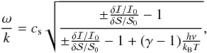 (1)where ω/k is the phase speed, cs is the internal sound speed, δℐ is the amplitude of the intensity perturbation,
  is the amplitude of the area perturbation, ℐ0 is the mean intensity,
  is the mean area, γ is the ratio of specific heats, h is the Planck constant, kB is the Boltzmann constant, T is the temperature of the plasma inside the flux tube, and ν is the frequency at which the observation was taken. The ± in the formula arise since this is a quadratic equation, but a unique solution is found when also using the phase differences. The most important parameter, from an observational point of view, is the dimensionless amplitude ratio A, which is given by
 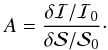 (2)This parameter is very important since it relates the amplitude of the oscillation directly to the phase speed using Eq. (1).
2.2. Data analysis method
In this section, we describe the data analysis method and afterwards test the validity using synthetic data. The first step is the thresholding routine in which we calculate both the area and the intensity of the magnetic pore. The magnetic pore is constituted by the pixels that have a photon count of less than 3σ of a quiet-Sun region within the same field of view (FOV; Morton et al. 2011; Dorotovič et al. 2014). The total intensity is the sum of all the photon counts within the magnetic pore at each time step. We have summed the intensity over all the pixels inside the pore at each time step and we implicitly assume that the magnetic pore consists of the same plasma elements at each time step, therefore we are working with a Lagrangian intensity variation. This thresholding routine results in both an area and intensity time series. The next step is to use a wavelet analysis on the area and intensity time series to identify time intervals of strong oscillatory power in both the area and intensity time series. These time intervals of strong power are then processed by a fast Fourier transform (FFT) to find the phase difference between the area and intensity time series and the amplitude of the perturbations in both time series. The phase difference is used to identify the wave mode, i.e. fast or slow. The amplitude is used to find the phase speed by using Eq. (1). This entire method is summarised in Table 1.
A summary of the key steps in the data analysis method.
2.3. Synthetic data
To test the validity of this method we generated a set of data using the cylindrical model representing a magnetic pore in the photosphere. This data set consists of a series of intensity images with a pore in the FOV with a noise of 10% of the pixel value, as can be seen in Fig. 1. This synthetic data set is not intended to be an accurate representation of the solar photosphere. Therefore there is no granulation present in this data set. This synthetic data set represents a uniform flux tube in a uniform atmosphere superposed with linear MHD waves and synthetic noise. Hence, this data set is an ideal example to test the validity of the data analysis method since the structure we analyse is identical to the structure we studied analytically. The generation of the data is carried out by the following steps. First, we generate a fixed (x0,y0) grid with a uniform spacing of about 50 km. On each of the grid nodes we compute the Lagrangian displacement ξx(x0,y0) and ξy(x0,y0) and the Eulerian intensity perturbation I′(x0,y0). The Eulerian intensity perturbation I′ can be found in e.g. Moreels et al. (2013) in their Eq. (5) when applied to uniform flux tubes. Second, we construct an advected grid (x1,y1) by moving the grid nodes according the Lagrangian displacement ξx and ξy, i.e. (x1,y1) = (x0,y0) + (ξx(x0,y0),ξy(x0,y0)). The intensity perturbation I′(x1,y1) is not changed, and it moves with the grid node. Third, the advected grid (x1,y1) is linearly interpolated to a new fixed (x2,y2) grid with a uniform grid spacing of about 50 km since solar observations use a fixed grid. Linear interpolation is used to minimise the amount of smoothing near the pore boundary. The intensity perturbation I′(x1,y1) is also linearly interpolated to the new fixed grid. Fourth, a Gaussian noise is added to each pixel indepently per time step. The standard deviation of the noise was set at 10%. The reason for choosing 10% noise level is that the variations in the actual observed intensity (see Fig. 5) are of the order 5−20%. To ensure that the conclusions from the synthetic data were applicable to the observations, we used a magnetic pore with a similar radius as in the observations and a similar resolution. In this data set, we modelled different oscillations, i.e. slow/fast modes and surface/body modes. The amplitude of the different oscillations is chosen such that the density perturbation is approximately 5% of the background density. This ensures that the wave modes are in the linear regime. The perturbation amplitude resulted in radial changes at the flux tube boundary between 1−10 km, i.e. well below the resolution of the data, which is about 50 km. Intuitively we expect that our data analysis method will overestimate the change in area since the pore might have crossed a pixel boundary, while not having moved the complete length of the pixel.
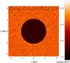 |
Fig. 1 One slice from the synthetic data set representing a magnetic pore in a model solar photosphere. The colour scale is the intensity. The hatched region at the top indicates the region that was used as the quiet-Sun region for the thresholding routine. |
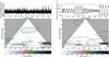 |
Fig. 2 Top image: time series for the area (left) and intensity (right), bottom: wavelet power spectrum of the time series. The grey area is the region where boundary issues from the wavelet process can occur, known as the cone of influence. The coloured lines indicate the time intervals used in the Fourier analysis and are placed at the period found from Fourier analysis. |
There are several physical effects we investigate. First, does the wavelet analysis identify the correct time intervals of strong power? Second, how could the effect of the sub-resolution area change be observed? Third, what are the errors on the inferred phase speed? Fourth, what is the effect of clouds on the thresholding routine? This is a relevant question because the observations we want to study are ground-based (see Sect. 3). This question is addressed in Appendix A in detail.
To test the validity of the data analysis method described, we focussed on the data set with no clouds. We first discuss step 2 from Table 1, i.e. the wavelet analysis. We determined the area from the thresholding routine and determined the Lagrangian intensity at time t by summing the intensity over all the pixels inside the flux tube at that time (i.e. pixels with intensity below the threshold). Since the intensity is calculated by summing over a group of pixels, the noise effects are very small. The resulting time series are first analysed with a wavelet analysis to find time intervals of strong power in both area and intensity. The results can be seen in Fig. 2. The top of the figures show the raw time series. As mentioned, there is little noise in the intensity and the oscillations are clearly visible with the naked eye. The area has a lot more noise for two reasons. First, there is no summing over pixels when measuring the area and, therefore, the noise is not cancelled in that way. Second, the radial displacement is smaller than the resolution, meaning that there is only a very small change in the measured area.
The coloured horizontal lines in Fig. 2 coincide with the time intervals of strong power of the intensity time series. The time intervals of strong power in the area mostly coincide with time intervals of strong power for the intensity, i.e. all periods around or below 10 min in the area time series match with corresponding regions in the intensity time series. There are several regions in the intensity time series with periods around or below 10 min that do not have a counterpart in the area time series, which happens because the noise dominates over the small radial displacement. For periods above 10 min there are no corresponding regions in both area and intensity time series, i.e. no spurious solutions were found. It is appropriate to mention here that the thresholding routine did have some problems because of the sub-resolution nature of the area change, namely the routine did not correctly detect the contraction of the pore; it only detected the expansion of the pore. In other words the magnitude of the area perturbation has been underestimated by a factor of 2. This is due to the sub-resolution change of the area as well as the generation process for the synthetic data. In generating the synthetic data, we have interpolated the intensity at the pore boundary, which smooths the sharp jump at the boundary. We believe this also contributes to not detecting the contractions of the pore. This concludes the discussion of step 2 from Table 1.
The input parameters of the wave modes in the synthetic data, combined with the results of the FFT analysis on the synthetic data.
Next, we discuss step 3 from Table 1, i.e. the Fourier analysis. The time series are divided into the time intervals of strong power, based on the intensity time series since this has less noise. In total we now have 14 time series, 7 for intensity and 7 for area, each representing a different oscillation mode. Before Fourier analysing these 14 time series, we mention the actual input parameters of the simulations, see Table 2. Table 2 lists the type of wave, the time interval where it appears, the period, the amplitude ratio A, and the phase speed. Of course, the theoretical period is the same for both the intensity and the area oscillation. The phase speed mentioned in the table is the actual input value and not the result of using Eq. (1) on the amplitude ratio A. If, however, we calculate the phase speed using the amplitude ratio, we find a very good agreement with a difference of about 1%, which can be explained by numerical round-off errors.
The results from the Fourier analysis can be found in Table 2. As expected, the Fourier analysis performed well on the intensity time series, with a clear peak in the power spectrum. This period matches the value of the input, in Table 2, with a maximum error of about 10%. The Fourier analysis did not perform as well with the area time series. For certain time intervals there was no peak present around the expected period (there were also no clear peaks at other periods). We denoted those time intervals with “not found”. In one other case, the noise was dominant over the perturbation and we had to ignore the periods under 60 s to find the appropriate peak in the power spectrum; that case is indicated with an asterix. The error estimate for the period is based on the broadness of the peak in the Fourier power spectrum.
We continue with step 4 from Table 1, i.e. the wave mode identification. As mentioned before, the phase difference between the area and the intensity perturbations for slow modes should be around zero degrees and around 180 deg for fast modes. The phase difference found from the synthetic data indeed exhibits the correct behaviour, except for the slow body mode, which is 70 deg, although it should be zero degrees. Using cross-correlation to analyse the area and intensity for that slow body mode, we found that there was a phase differences of 45 deg. We further analysed this case to find out why the phase difference is clearly non-zero. When we did the analysis again with less noise, 1% of the pixel value, cross-correlation showed a phase difference of zero degrees. This, again, confirms the problem that determination of the area is very sensitive to noise effects and care needs to be taken in analysing the observations.
Finally, we discuss step 5 from Table 1, i.e. determining the phase speed. From a seismological point of view the most important value is the amplitude ratio A, since this value determines (together with the equilibrium parameters) the phase speed of the oscillation. On the Sun, however, the equilibrium parameters and the driver of the wave determine the phase speed and thus finding the phase speed reveals information about the structure of the magnetic pore. If we compare the amplitude ratio A from the Fourier analysis with the exact input values, we find that the values have similar orders of magnitude with errors up to a factor of 10 for the slow surface modes. The Fourier analysis also underestimates the magnitude of the area perturbations. For some cases, the Fourier analysis reported a magnitude of only 1 pixel, while it should have been 10 pixels. This is caused by the effects of noise on the area time series. The combination of underestimating the area variations in both the Fourier analysis and in the thresholding routine results in area amplitudes that compare with the actual input values, while we expected the amplitudes to be overestimated. The error for the amplitude parameter is quite high. However, how does this error propagate into the inferred phase speed (using Eq. (1))? Looking at the phase speed and comparing with the actual values, we find that the values match with a maximum error of 15%. This is, in our opinion certainly a very acceptable margin for error, especially considering the 10% noise level. The largest errors are both for slow surface modes, for which the actual phase speed is not in the error estimate interval. Other modes, i.e. slow body modes and fast modes, do not have this error. The actual input phase speed is for all cases inside the error estimate interval. An explanation for this behaviour is yet to be found, but that is beyond the scope of this paper.
Because this data analysis method is not completely automated, i.e. the time series have to be divided into smaller time series manually, it is very time consuming to use a Monte Carlo method to estimate the uncertainty of the data analysis method. However, when only simulating one wave mode, the time series does not need to be divided and the data analysis method is fully automated. We chose a fast surface mode and a slow body mode to calculate the uncertainty interval using a Monte Carlo method. The fast surface mode occurs in the synthetic data during the time interval [ 0,8.1 ] and the slow body mode occurs during the time interval [ 95.4,114.4 ]. For both the fast mode and the slow body mode, 1000 time series are generated each with their independent noise as described above. The data analysis method (without steps 2 and 3) is applied to each time series. Thus, there are 1000 values values for both the fast surface mode and the slow body mode for the area and intensity periods, the phase difference, the amplitude ratio, and the phase speed. These 1000 values are then sufficient to establish a mean value and a proper uncertainty estimate, which are reported in Table 2. There is no uncertainty estimate for the intensity period because the perturbation is very clear, also with the naked eye, and as such the Fourier analysis picks out the same period in all 1000 time series. As can be seen in Table 2, the uncertainty intervals for the fast surface mode are quite narrow. The uncertainty intervals for the slow body mode are wider. The area period is not the most important parameter because the intensity period is clear. The phase difference has a wide spread, but this slow body mode is the case that was discussed earlier in which the phase difference was clearly non-zero because of noise effects. The phase speed still has a limited uncertainty interval.
Our results from the synthetic data clearly show that the method we described in Table 1 works with an acceptable margin of error on the resulting phase speed.
3. Data collection
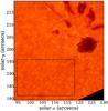 |
Fig. 3 Observed active region. The large pore at the top of the FOV is the subject of this article. The contour shows the area of the thresholded pore boundary. The hatched region is the quiet-Sun region used in calculating the threshold for intensity. |
We collected the ground-based data analysed here with the CRisp Imaging SpectroPolarimeter (CRISP) instrument (Scharmer et al. 2008), situated at the 1-m Swedish Solar Telescope (SST), La Palma between 07:23 UT and 08:28 UT on 2012 June 22. The region observed was within NOAA 11510, centred on a large pore. We took the data in Hα with a core line position at 656.3 nm, and returned the line scans to the left and right of the line core with a −0.1032, −0.0774 and 0.1032 shift. The FOV covers 68′′ by 68′′. Next, we reconstructed the data with the Multi-Object Multi-Frame Blind Deconvolution (MOMFBD) technique (for details see van Noort et al. 2005) giving an overall cadence of two seconds and a spatial resolution of 0.12′′.
Following Morton et al. (2011) and Dorotovič et al. (2014), and as explained in Sect. 2.2, we defined the pixels that constitute the magnetic pore as pixels that have a photon count less than 3σ of the quiet-Sun region within the same FOV. Figure 3, shows the boundary of the pore that was calculated by the algorithm and the hatched region is the quiet-Sun region used to define the threshold limit. The darker region just to the right of the pore boundary is a feature that decays in time and is therefore not a part of the pore. The thresholding method is not entirely accurate because the pore boundary is reasonably continuous, and there tends to be a region of several pixels between the pore and the quiet-Sun. Despite this limitation, this is a more natural method of calculating the area of magnetic structures than an arbitrary intensity limit. The total intensity is the sum of all the photon counts within the magnetic pore at each time step.
Figure 4 shows the area time series, which is a result of applying the thresholding routine on the observational data. Clearly noticeable are the almost discontinuous jumps at the start of the time series. We are confident the cause for these jumps were clouds passing over the telescope. When comparing the jumps in Fig. 4 with those in Appendix A (Fig. A.2), it becomes clear that clouds could indeed explain the jumps at the start of the observations. Therefore, while for the majority of the time window, the seeing was considered to be very good, the first 10 min and the last 15 min had highly variable seeing. As is explained in Appendix A and, as can be seen from Fig. 4, this introduced artifacts into the cross-sectional area and total intensity signals. For this reason, we trimmed the data leaving just over 35 min of high-quality data.
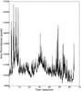 |
Fig. 4 Area time series of the full 1 h data set. Notice the almost discontinuous jumps in the first 10 min of the time series. |
To extract the relevant information required, i.e. both the phase and magnitude of the wave perturbations in the area and intensity time series, wavelets were used in conjunction with the FFT. We used the wavelet algorithm to identify the dominant periods within the area and intensity, and when these periods appear and disappear from the time series. Then, the two signals were divided into segments that contained these dominant periods and the amplitudes of the oscillations were calculated using the FFT for these segments individually. This approach is also summarised in Table 1.
4. Analysis of the observations
We now apply the method outlined in Table 1 to the actual observations. The wavelet power spectrum is shown in Fig. 5 for both the area and intensity perturbation time series. The black line shows the 95% confidence limit and the grey region is where wavelet edge effects become important and is referred to as the cone of influence (COI). We focus on the time intervals outside the COI.
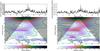 |
Fig. 5 Top image: time series for the area (left) and the intensity (right), bottom: wavelet power spectrum of the time series for the observed pore. The grey area is the region, known as the cone of influence, where boundary issues from the wavelet process can occur. The blue lines indicate the time intervals used in the Fourier analysis and are placed at the period found from Fourier analysis. |
Results of the data analysis on the observations.
When studying both wavelet plots different regions of strong power are obvious. We now list all the regions we selected for the Fourier analysis: 8 to 20 min with 6.5 min period, 10 to 17 min with 3 min period, 10 to 35 min with 2 and 1.5 min periods, and 25 to 35 min with 2 and 1.5 min periods. The last time interval is not mentioned in Table 3 because the results are almost identical to the time interval of 10 to 35 min with 2 and 1.5 min periods. The regions have been indicated by blue coloured horizontal lines in Fig. 5. Table 3 shows the results of the Fourier analysis on all these time intervals. It is immediately clear that all phase differences are close to zero, meaning that we are observing slow waves (cf. Moreels et al. 2013).
Using Eq. (1) and the amplitude ratio A, we also calculated the phase speed. In cases with multiple solutions, we chose the phase speed corresponding to a slow mode. There were also cases with no real solution to Eq. (1). We remedied this by dividing the amplitude of the area perturbations by two. Dividing the area amplitude by two is not a random choice. In the observational data we found that the change in radius of the observed pore is smaller than one pixel, i.e. the change in radius is sub-resolution. This was also the case for the synthetic data in Sect. 2.2, although the difference between the spatial resolution and the radial displacement of the pore boundary in the observational data is not as extreme as in the synthetic data. In Sect. 2.2 we mentioned that we expected the area amplitude to be overestimated because the radial displacement is smaller than the resolution of the intensity image. We also mentioned that the thresholding routine did not detect the contractions of the synthetic pore, which resulted in underestimating the synthetic area amplitude by a factor of two. This underestimation of the synthetic area amplitude in the thresholding routine led to correct phase speed values for the synthetic data. We believe this underestimation in the synthetic data is caused by our method of generating the synthetic data, i.e. using interpolation at the pore boundary. Of course, in the observational data there is no interpolation of intensity at the pore boundary, therefore the underestimation of the area amplitude does not occur and the area amplitude is overestimated. To correct for the potentially misleading results on the phase speed this can have, we divided the area amplitude by a factor of two. The error bars in Table 3 are due to this uncertainty in the amplitude of the area perturbation. The lower values (of the amplitude ratio A) are taken with , the middle values (of the amplitude ratio A) with  , and the upper values (of the amplitude ratio A) with
  .
.
The resulting phase speeds are of the order 5 km s-1, which are smaller than the internal sound speed, as should be the case for slow modes. However, we do not know if these waves are standing or propagating, therefore the phase speed does not necessarily represent an upwards propagation speed. If we look at the period, or the kR values, or the wavelength, it is easy to get the impression that we might be observing overtones of a fundamental mode with period 6.5 min. As explained in Dorotovič et al. (2014) the use of an ideal flux tube would lead to harmonic period ratios as P1/P2 = 2, P1/P3 = 3, and so on. We indeed have the same harmonic period ratios. There has also been research done to see how the period ratios change under the influence of more realistic equilibrium models (Luna-Cardozo et al. 2012), which shows that certain density profiles can increase or decrease the harmonic period ratios.
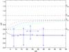 |
Fig. 6 Phase speed diagram of wave modes under photospheric conditions. We use as equilibrium parameters cA,i = 1.3cs,i, cA,e = 0.1cs,i, and cs,e = 1.1cs,i. The external Alfvén speed is not indicated in the graph because no modes with real frequencies appear in that vicinity. The modes with phase speeds between cT,i and cs,i are body modes and the other mode is a surface mode. We only plotted four body modes, while there are infinitely many radial overtones. There are no non-leaky fast modes. The blue circles indicate the location of the observations and the blue triangles are the uncertainty bars. |
Before using the oscillations as a tool for seismology we first discuss a physical mechanism to generate these standing waves. A possible mechanism for these standing waves is that of the chromospheric resonator above sunspot umbrae (Botha et al. 2011). We have already mentioned that magnetic pores behave in a very similar manner to sunspot umbrae, meaning that there could also be a chromospheric resonator above magnetic pores. The chromospheric resonator or chromospheric cavity is the region above the photosphere up to the transition region, i.e. about 2 Mm in length. This length scale matches the wavelength of the fundamental mode in the observations, see Table 3. The theory of a chromospheric resonator has also been used as a possible explanation for the observed long period waves in the solar corona (Yuan et al. 2011).
Finally, we can use the phase speed and the kR values of the observed waves to estimate equilibrium parameters of the magnetic pore, i.e. using MHD seismology. Using harmonics for seismology has been carried out by, e.g. Andries et al. (2005), on kink oscillations in the corona. Since we know the position of the observations in the phase diagram of MHD waves in a magnetic cylinder, we know that one or more of the dispersion curves need to overlap with the observations. In Fig. 6 we plotted the observations with their uncertainties both in phase speed and in kR value. Next, we obtained a set of equilibrium parameters such that all of the observations agree with one of the dispersion curves, and in this case the curve for the slow surface mode. A possible, but not unique, set of equilibrium parameters that fits with the observations are cA,i = 1.3cs,i, cA,e = 0.1cs,i, and cs,e = 1.1cs,i. From the observations we already knew the difference between internal and external sound speed, but we now also have an estimate for the Alfvén speeds. This set of equilibrium parameters means a plasma β around 0.7 inside the flux tube and around 150 outside the flux tube. The high value outside just indicates that there is a very weak magnetic field outside the flux tube. This is certainly not the only possible combination of equilibrium parameters that fit the observations. We investigated different combinations of equilibrium parameters and found that the external Alfvén speed cA,e between [ 0.0,0.7cs,i ], external sound speed cs,e between [ cs,i,1.5 [ cs,i, and internal Alfvén speed cA,i between [ cs,e,2.0cs,i ] yielded reasonable fits to the data points (which have large uncertainties). Most of these combinations have in common that the observations are slow surface waves rather than body waves. Also common in the possible parameters is the low external Alfvén speed, which indicates a weak magnetic field outside the magnetic pore. The generation of slow surface sausage modes could be related to the excitation by slow downdrafts, such as those simulated by Kato et al. (2011). These slow downdrafts also explain the surface nature of the waves, since the driver of the waves is situated mainly outside the flux tube. The generation of slow sausage modes can also be caused by other phenomena, e.g. granular buffeting or convective cell motions (Fedun et al. 2011a,b).
5. Conclusions
We investigated axisymmetric modes in solar magnetic pores. For the first time, we estimated the phase speed of waves in solar magnetic pores using only intensity images at one height. In the literature we only found estimates of phase speeds when using multiple heights in observations or using LOS velocity or LOS magnetic field information. The observations were taken using the CRISP instrument located at the SST in La Palma. Using a thresholding routine, we obtained both the cross-sectional area of the pore and the Lagrangian intensity perturbation. With a combination of wavelet and Fourier analysis, we identified several oscillations in both area and intensity. Using MHD theory, we discovered that the oscillations are standing slow surface modes with a phase speed around 5 km s-1. The standing nature of these modes can be explained by the chromospheric resonator model and the three harmonic overtones of the fundamental 6.5 min period. The wavelength of the fundamental mode also matches with the length scale of the chromospheric cavity, i.e. about 2 Mm. Using the phase speed and kR value in combination with the dispersion diagram we were able to identify ranges of plausible equilibrium parameters. We found the external Alfvén speed cA,e between [ 0.0,0.7cs,i ], external sound speed cs,e between [ cs,i,1.5 [ cs,i, and internal Alfvén speed cA,i between [ cs,e,2.0cs,i ]. For most of these equilibrium configurations this shows that the observed waves are surface waves with a weak magnetic field outside the pore.
We verified our proposed data analysis method (see Table 1) using synthetic observations. The synthetic observations are normalised such that the density perturbation is about 5% of the background density, i.e. linear perturbations. This resulted in small radial displacements well below the spatial resolution of the data. We investigated three effects, namely the detection of oscillations in the data using wavelet and Fourier analysis, the accuracy of MHD seismology, and the effect of clouds on the thresholding routine. This last effect has been explained in Appendix A. We also mention that our proposed data analysis method could easily be tested on more realistic numerical simulations.
First, we tested the accuracy of the wavelet and Fourier analysis. We discovered that the analysis does not result in the detection of all area oscillations present in the data, but there are also no spurious oscillations found from the analysis. The fact that we did not detect all oscillations present is purely because, in some cases, the radial displacements are ten times smaller than the spatial resolution of the observations. This means that the pore boundary has not shifted an entire pixel and therefore this shift is hard to detect. We did find all oscillations in intensity because we summed over all the pixels that are inside the pore and noise effects are strongly reduced. Second, we checked how accurate the seismology was in distinguishing the wave mode and in determining the phase speed. Investigating the cases where an oscillation was identified, we found that in all but one case the method correctly identified the wave mode (i.e. fast or slow), except for the slow body mode. This happened because of noise effects, showing that noise can also change the phase behaviour of the wave mode. Determining the phase speed was quite successful with errors up to 15% of the original input value. This is a good result because the uncertainty due to seismology is at the same level of the noise in the data (10%). Finally, we investigated the effect of clouds passing over the telescope since this occurred during the observation. The result was very clear: the clouds dramatically interfered with the thresholding routine and resulted in unphysical data for both intensity and area. We found no way to account for this process and, therefore, dropped the data where clouds passed over the telescope.
We believe this work forms the basis of a future time-dependent and dynamical magneto-seismological study of magnetic pores. This work can be used as a basis for modelling how time and space dependent magnetic fields, density structures, pressure changes, etc. influence both the wave modes and the observables (i.e. periods, cross-sectional area, intensity, etc.) of those wave modes.
Online material
Appendix A: The influence of clouds on the calculation of the area
In Sect. 2.3 we examined the effect of changing seeing conditions, i.e. clouds. We modelled the clouds as having two effects, namely a decrease of the intensity due to scattering, and a smoothing over pixels also due to scattering. The decrease in intensity due to clouds is 10% of the pixel value and the pixels are linearly smoothed over the neighbouring pixels only. This cloud was then turned on and off in a periodic fashion. The visual result can be seen in Fig. A.1. The result is as expected, the image looks blurry when compared to the non-cloudy image, i.e. Fig. 1. However, does this have an effect on the thresholding routine determining the area of the pore? The result can be seen in Fig. A.2. One can clearly see that clouds have a major impact on the thresholding routine. We tried to remedy this, but the smoothing over pixels is very hard to correct for. We realise that the clouds employed are unrealistic in the sense that they spontaneously appear in the entire FOV and that they are periodic. However the fact that clouds spontaneously appear is not a real concern since the small viewing aperture results in an almost immediate the cloud cover. Clouds are non-periodic but even one cloud is enough to deteriorate the data at that time. This is the reason that we decided to discard certain time intervals in the observations.
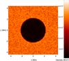 |
Fig. A.1 One slice from the data set representing a magnetic pore in the solar photosphere with a cloud introducing seeing effects. The colour scale is the intensity. |
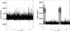 |
Fig. A.2 Area of the simulated magnetic pore based on the thresholding routine. Left: area without cloud effects. Right: area with cloud effects. |
Acknowledgments
R.E. acknowledges M. Kéray for patient encouragement and is also grateful to NSF, Hungary (OTKA, Ref. No. K83133). This work is supported by the UK Science and Technology Facilities Council (STFC). Wavelet power spectra were calculated using a modified computing algorithm of wavelet analysis, the original of which was developed and provided by C. Torrence and G. Compo, and is available at URL: http://paos.colorado.edu/research/wavelets/. The CRisp Imaging SpectroPolarimeter instrument at the Swedish 1 m Solar Telescope is operated on the island of La Palma by the Institute for Solar Physics of the Royal Swedish Academy of Sciences in the Spanish Observatorio del Roque de los Muchachos of the Instituto de Astrofsica de Canarias. We would like to thank L. Rouppe v. d. Voort (Institute of Theoretical Astrophysics, University of Oslo) and J. de la Cruz Rodriguez (University of Uppsala, Sweden) for data reductions with MOMFBD for SST/CRISP. M.M. and T.V.D. have received funding from the Odysseus programme of the FWO-Vlaanderen and from the EU’s Framework Programme 7 as an ERG with grant number 276808. The research was conducted in the framework of Belspo’s IAP P7/08 CHARM and the GOA-2015-014 of the Research Council of the KU Leuven. GV thanks the Leverhulme Trust (UK).
References
- Andries, J., Arregui, I., & Goossens, M. 2005, ApJ, 624, L57 [NASA ADS] [CrossRef] [Google Scholar]
- Andries, J., Van Doorsselaere, T., Roberts, B., et al. 2009, Space Sci. Rev., 149, 3 [NASA ADS] [CrossRef] [Google Scholar]
- Banerjee, D., Erdélyi, R., Oliver, R., & OShea, E. 2007, Sol. Phys., 246, 3 [NASA ADS] [CrossRef] [Google Scholar]
- Bloomfield, D. S., Lagg, A., & Solanki, S. K. 2007, ApJ, 671, 1005 [NASA ADS] [CrossRef] [Google Scholar]
- Bogdan, T. J., & Judge, P. G. 2006, Roy. Soc. London Philos. Trans. Ser. A, 364, 313 [Google Scholar]
- Bogdan, T. J., Carlsson, M., Hansteen, V. H., et al. 2003, ApJ, 599, 626 [NASA ADS] [CrossRef] [Google Scholar]
- Botha, G. J. J., Arber, T. D., Nakariakov, V. M., & Zhugzhda, Y. D. 2011, ApJ, 728, 84 [NASA ADS] [CrossRef] [Google Scholar]
- Cally, P. S. 1986, Sol. Phys., 103, 277 [NASA ADS] [CrossRef] [Google Scholar]
- De Moortel, I., & Nakariakov, V. M. 2012, Roy. Soc. London Philos. Trans. Ser. A, 370, 3193 [Google Scholar]
- Dorotovič, I., Erdélyi, R., & Karlovský, V. 2008, in Proc. IAU Symp. 247, eds. R. Erdélyi, & C. A. Mendoza-Briceño (Cambridge University Press), 351 [Google Scholar]
- Dorotovič, I., Erdélyi, R., Freij, N., Karlovský, V., & Márquez, I. 2014, A&A, 563, A12 [NASA ADS] [CrossRef] [EDP Sciences] [Google Scholar]
- Edwin, P. M., & Roberts, B. 1983, Sol. Phys., 88, 179 [NASA ADS] [CrossRef] [Google Scholar]
- Erdélyi, R., & Goossens, M. 2011, Space Sci. Rev., 158, 167 [NASA ADS] [CrossRef] [Google Scholar]
- Erdélyi, R., & Verth, G. 2007, A&A, 462, 743 [NASA ADS] [CrossRef] [EDP Sciences] [Google Scholar]
- Fedun, V., Shelyag, S., & Erdélyi, R. 2011a, ApJ, 727, 17 [NASA ADS] [CrossRef] [Google Scholar]
- Fedun, V., Shelyag, S., Verth, G., Mathioudakis, M., & Erdélyi, R. 2011b, Ann. Geophys., 29, 1029 [Google Scholar]
- Freij, N., Scullion, E. M., Nelson, C. J., et al. 2014, ApJ, 791, 61 [NASA ADS] [CrossRef] [Google Scholar]
- Fujimura, D., & Tsuneta, S. 2009, ApJ, 702, 1443 [NASA ADS] [CrossRef] [Google Scholar]
- Jess, D. B., Reznikova, V. E., Van Doorsselaere, T., Keys, P. H., & Mackay, D. H. 2013, ApJ, 779, 168 [NASA ADS] [CrossRef] [Google Scholar]
- Kato, Y., Steiner, O., Steffen, M., & Suematsu, Y. 2011, ApJ, 730, L24 [NASA ADS] [CrossRef] [Google Scholar]
- Khomenko, E., Collados, M., & Felipe, T. 2008, Sol. Phys., 251, 589 [NASA ADS] [CrossRef] [Google Scholar]
- Kobanov, N. I., Kolobov, D. Y., & Makarchik, D. V. 2006, Sol. Phys., 238, 231 [NASA ADS] [CrossRef] [Google Scholar]
- Luna-Cardozo, M., Verth, G., & Erdélyi, R. 2012, ApJ, 748, 110 [NASA ADS] [CrossRef] [Google Scholar]
- Marsh, M., & Walsh, R. 2008, ApJ, 643, 540 [Google Scholar]
- Moreels, M. G., & Van Doorsselaere, T. 2013, A&A, 551, A137 [NASA ADS] [CrossRef] [EDP Sciences] [Google Scholar]
- Moreels, M. G., Goossens, M., & Van Doorsselaere, T. 2013, A&A, 555, A75 [NASA ADS] [CrossRef] [EDP Sciences] [Google Scholar]
- Morton, R. J., Erdélyi, R., Jess, D. B., & Mathioudakis, M. 2011, ApJ, 729, L18 [NASA ADS] [CrossRef] [Google Scholar]
- Ofman, L. 2005, Space Sci. Rev., 120, 67 [NASA ADS] [CrossRef] [Google Scholar]
- Osterbrock, D. E. 1961, ApJ, 134, 347 [NASA ADS] [CrossRef] [Google Scholar]
- Parnell, C. E., & De Moortel, I. 2012, Roy. Soc. London Philos. Trans. Ser. A, 370, 3217 [Google Scholar]
- Reznikova, V. E., & Shibasaki, K. 2012, ApJ, 756, 35 [NASA ADS] [CrossRef] [Google Scholar]
- Roberts, B., & Mangeney, A. 1982, MNRAS, 198, 7P [NASA ADS] [CrossRef] [Google Scholar]
- Rosenthal, C. S., Bogdan, T. J., Carlsson, M., et al. 2002, ApJ, 564, 508 [NASA ADS] [CrossRef] [Google Scholar]
- Rouppe van der Voort, L. H. M., Rutten, R. J., Sütterlin, P., Sloover, P. J., & Krijger, J. M. 2003, A&A, 403, 277 [NASA ADS] [CrossRef] [EDP Sciences] [Google Scholar]
- Sakurai, T., Goossens, M., & Hollweg, J. V. 1991, Sol. Phys., 133, 227 [NASA ADS] [CrossRef] [Google Scholar]
- Scharmer, G. B., Narayan, G., Hillberg, T., et al. 2008, ApJ, 689, L69 [NASA ADS] [CrossRef] [Google Scholar]
- Taroyan, Y., & Erdélyi, R. 2009, Space Sci. Rev., 149, 229 [NASA ADS] [CrossRef] [Google Scholar]
- Terradas, J., Oliver, R., & Ballester, J. 2004, ApJ, 614, 435 [NASA ADS] [CrossRef] [Google Scholar]
- Torrence, C., & Compo, G. 1998, Bull. Amer. Meteor. Soc., 79, 61 [CrossRef] [Google Scholar]
- van Noort, M., Rouppe van der Voort, L., & Löfdahl, M. G. 2005, Sol. Phys., 228, 191 [NASA ADS] [CrossRef] [Google Scholar]
- Vigeesh, G., Hasan, S. S., & Steiner, O. 2009, A&A, 508, 951 [NASA ADS] [CrossRef] [EDP Sciences] [Google Scholar]
- Vigeesh, G., Fedun, V., Hasan, S., & Erdélyi, R. 2012, ApJ, 755, 18 [NASA ADS] [CrossRef] [Google Scholar]
- Yuan, D., Nakariakov, V. M., Chorley, N., & Foullon, C. 2011, A&A, 533, A116 [NASA ADS] [CrossRef] [EDP Sciences] [Google Scholar]
- Yuan, D., Sych, R., Reznikova, V. E., & Nakariakov, V. M. 2014, A&A, 561, A19 [NASA ADS] [CrossRef] [EDP Sciences] [Google Scholar]
- Zaitsev, V. V., & Stepanov, A. V. 1975, Issled. Geomagn. Aeron. Fiz. Solntsa, 37, 3 [Google Scholar]
All Tables
The input parameters of the wave modes in the synthetic data, combined with the results of the FFT analysis on the synthetic data.
All Figures
|
Fig. 1 One slice from the synthetic data set representing a magnetic pore in a model solar photosphere. The colour scale is the intensity. The hatched region at the top indicates the region that was used as the quiet-Sun region for the thresholding routine. |
| In the text | |
|
Fig. 2 Top image: time series for the area (left) and intensity (right), bottom: wavelet power spectrum of the time series. The grey area is the region where boundary issues from the wavelet process can occur, known as the cone of influence. The coloured lines indicate the time intervals used in the Fourier analysis and are placed at the period found from Fourier analysis. |
| In the text | |
|
Fig. 3 Observed active region. The large pore at the top of the FOV is the subject of this article. The contour shows the area of the thresholded pore boundary. The hatched region is the quiet-Sun region used in calculating the threshold for intensity. |
| In the text | |
|
Fig. 4 Area time series of the full 1 h data set. Notice the almost discontinuous jumps in the first 10 min of the time series. |
| In the text | |
|
Fig. 5 Top image: time series for the area (left) and the intensity (right), bottom: wavelet power spectrum of the time series for the observed pore. The grey area is the region, known as the cone of influence, where boundary issues from the wavelet process can occur. The blue lines indicate the time intervals used in the Fourier analysis and are placed at the period found from Fourier analysis. |
| In the text | |
|
Fig. 6 Phase speed diagram of wave modes under photospheric conditions. We use as equilibrium parameters cA,i = 1.3cs,i, cA,e = 0.1cs,i, and cs,e = 1.1cs,i. The external Alfvén speed is not indicated in the graph because no modes with real frequencies appear in that vicinity. The modes with phase speeds between cT,i and cs,i are body modes and the other mode is a surface mode. We only plotted four body modes, while there are infinitely many radial overtones. There are no non-leaky fast modes. The blue circles indicate the location of the observations and the blue triangles are the uncertainty bars. |
| In the text | |
|
Fig. A.1 One slice from the data set representing a magnetic pore in the solar photosphere with a cloud introducing seeing effects. The colour scale is the intensity. |
| In the text | |
|
Fig. A.2 Area of the simulated magnetic pore based on the thresholding routine. Left: area without cloud effects. Right: area with cloud effects. |
| In the text | |
Current usage metrics show cumulative count of Article Views (full-text article views including HTML views, PDF and ePub downloads, according to the available data) and Abstracts Views on Vision4Press platform.
Data correspond to usage on the plateform after 2015. The current usage metrics is available 48-96 hours after online publication and is updated daily on week days.
Initial download of the metrics may take a while.