| Issue |
A&A
Volume 578, June 2015
|
|
|---|---|---|
| Article Number | A12 | |
| Number of page(s) | 9 | |
| Section | Numerical methods and codes | |
| DOI | https://doi.org/10.1051/0004-6361/201525971 | |
| Published online | 25 May 2015 | |
Multigroup radiation hydrodynamics with flux-limited diffusion and adaptive mesh refinement
1 Univ. Paris Diderot, Sorbonne Paris Cité, AIM, UMR 7158, CEA, CNRS, 91191 Gif-sur-Yvette, France
e-mail: This email address is being protected from spambots. You need JavaScript enabled to view it.
2 École Normale Supérieure de Lyon, CRAL, UMR CNRS 5574, Université de Lyon, 46 allée d’Italie, 69364 Lyon Cedex 07, France
3 School of Physics, University of Exeter, Exeter EX4 4QL, UK
Received: 26 February 2015
Accepted: 6 April 2015
Abstract
Context. Radiative transfer plays a crucial role in the star formation process. Because of the high computational cost, radiation-hydrodynamics simulations performed up to now have mainly been carried out in the grey approximation. In recent years, multifrequency radiation-hydrodynamics models have started to be developed in an attempt to better account for the large variations in opacities as a function of frequency.
Aims. We wish to develop an efficient multigroup algorithm for the adaptive mesh refinement code RAMSES which is suited to heavy proto-stellar collapse calculations.
Methods. Because of the prohibitive timestep constraints of an explicit radiative transfer method, we constructed a time-implicit solver based on a stabilized bi-conjugate gradient algorithm, and implemented it in RAMSES under the flux-limited diffusion approximation.
Results. We present a series of tests that demonstrate the high performance of our scheme in dealing with frequency-dependent radiation-hydrodynamic flows. We also present a preliminary simulation of a 3D proto-stellar collapse using 20 frequency groups. Differences between grey and multigroup results are briefly discussed, and the large amount of information this new method brings us is also illustrated.
Conclusions. We have implemented a multigroup flux-limited diffusion algorithm in the RAMSES code. The method performed well against standard radiation-hydrodynamics tests, and was also shown to be ripe for exploitation in the computational star formation context.
Key words: radiation: dynamics / radiative transfer / hydrodynamics / methods: numerical / stars: formation
© ESO, 2015
1. Introduction
Numerical studies of star formation are very demanding, as many physical mechanisms need to be taken into account (hydrodynamics, gravity, magnetic fields, radiative transfer, chemistry, etc.). Models are rapidly increasing in complexity, providing increasingly realistic interpretations of today’s highly advanced observations of protostellar systems, such as the recent groundbreaking images taken by the ALMA interferometer1. Radiative transfer plays an important role in star formation; it acts as a conduit to remove compressional heating during the initial stages of cloud collapse, enabling an isothermal contraction (Larson 1969; Masunaga et al. 1998), and it also inhibits cloud fragmentation in large-scale simulations (see e.g. Bate 2012). State-of-the-art simulations thus require the solutions to the full radiation magneto-hydrodynamics (RMHD) system of equations, and 3D simulations have only just recently become possible with modern computers (see e.g. Commerçon et al. 2011a; Tomida et al. 2013). In particular, including frequency dependent radiative transfer is essential in order to properly take into account the strong variations of the interstellar gas and dust opacities as a function of frequency (see e.g. Ossenkopf & Henning 1994; Li & Draine 2001; Draine 2003; Semenov et al. 2003; Ferguson et al. 2005). Three-dimensional calculations including full frequency-dependent radiative transfer are still out of reach of current computer architectures.
In order to overcome this difficulty, much effort has been spent in recent years developing mathematically less complicated, yet accurate approximations to the equations of radiative transfer. Such representations include diffusion approximations, the M1 model, short and long characteristics methods, and Variable Eddington Tensor descriptions. One of the simplest and most widely used is the flux-limited diffusion (FLD) approximation (Levermore & Pomraning 1981) that has been applied to many areas of physics and astrophysics.
These methods tend to drastically reduce computational cost, but still they are often integrated over all frequencies (also known as the grey approximation) as the multifrequency formalism remains too expensive. Only in recent years have multigroup methods (whereby the frequency-dependent quantities are binned into a finite number of groups and averaged over the group extents) appeared in numerical codes (Shestakov & Offner 2008; van der Holst et al. 2011; Vaytet et al. 2011, 2013b; Davis et al. 2012; Zhang et al. 2013, to mention a few) as a first step towards accounting for the frequency dependence of gas and dust quantities in calculations. Multigroup methods are very suited to astrophysics as they allow adaptive widths of groups, thus enabling the use of a small number of groups, concentrating frequency resolution where it is needed (i.e. mostly where opacity gradients are strong). Group boundaries are usually chosen once at the start of the simulations, but more complex schemes have also been written with moving adaptive borders (Williams 2005), as absorption and emission coefficients generally vary with the material temperature and density.
Commerçon et al. (2011b) implemented frequency-integrated FLD in the adaptive mesh refinement (AMR) code RAMSES (Teyssier 2002; Fromang et al. 2006), and devised an adaptive time-stepping scheme in a follow-up paper (Commerçon et al. 2014). In this third paper, we extend the method to a multigroup formalism. Even though multigroup effects were found to have only a small impact on 1D simulations of star formation (Vaytet et al. 2012, 2013a), they are expected to be enhanced in 3D where the optical thickness can markedly vary along different lines of sight (see Kuiper et al. 2011). Using a frequency-dependent method is also the only way to correctly model ultraviolet radiation from stars being absorbed by surrounding dust and re-emitted in the infrared. Finally, multigroup formalisms, compared to grey methods, are known to significantly affect the structures of radiative shocks (Vaytet et al. 2013b), alter energy transport in stellar atmospheres (Chiavassa et al. 2011), and are essential to neutrino transport in core collapse supernovae explosions (see e.g. Mezzacappa et al. 1998).
We first present the numerical method we have used, followed by a series of tests against analytical solutions, and we end with an application to the collapse of a gravitationally unstable cloud, comparing grey and multigroup results.
2. Numerical method
The FLD multigroup radiation hydrodynamics equations in the frame comoving with the fluid are ![Mathematical equation: \begin{eqnarray} \begin{array}{@{}l@{~~}c@{~~}l@{}} \partial_t \rho + \nabla \cdot [\rho {\vec u}] & = & 0 \\ \partial_t (\rho {\vec u}) + \nabla \cdot [\rho {\vec u} \otimes {\vec u} + P \mathbb{I}] & = & -\displaystyle \sum_{g=1}^{Ng}{\lambda_g \nabla E_g} \\ \partial_t E_{\mathrm{T}} + \nabla \cdot [{\vec u} (E_{\mathrm{T}} + P)] & = & \displaystyle \sum_{g=1}^{Ng}{\Bigg[- \mathbb{P}_g : \nabla {\vec u} - \lambda_g {\vec u} \cdot \nabla E_g } \\ && + \nabla \cdot \left(\displaystyle \frac{c\lambda_g}{\rho \kappa_{\mathrm{R}g}} \nabla E_g\right) \Bigg]\\ \partial_t E_g + \nabla \cdot [{\vec u} E_g] & = & - \mathbb{P}_g : \nabla {\vec u} + \nabla \cdot \left(\displaystyle \frac{c\lambda_g}{\rho \kappa_{\mathrm{R}g}} \nabla E_g\right) \\ && + \kappa_{\mathrm{P}g} \rho c \left(\Theta_g(T)-E_g\right) \\ && + \nabla {\vec u} : \displaystyle \int_{\nu_{g-1/2}}^{\nu_{g+1/2}}{\partial_\nu(\nu \mathbb{P}_\nu) {\rm d}\nu}, \end{array} \label{eq:rhd} \end{eqnarray}](/articles/aa/full_html/2015/06/aa25971-15/aa25971-15-eq2.png) (1)where c is the speed of light; ρ, u, P, and T are the gas density, velocity, pressure, and temperature, respectively; ET is the total energy
(1)where c is the speed of light; ρ, u, P, and T are the gas density, velocity, pressure, and temperature, respectively; ET is the total energy  (ϵ is the internal specific energy); and I is the identity matrix. We also define
  (2)where X = E, P, which represent the radiative energy and pressure inside each group g, which holds frequencies between νg−1 / 2 and νg + 1 / 2; Ng is the total number of groups; and Θg(T) is the energy of the photons having a Planck distribution at temperature T inside a given group. The coefficient λg is the flux-limiter, and κPg and κRg are the Planck and the Rosseland means of the spectral opacity κν inside a given group.
We employ a commonly used operator splitting scheme whereby the equations of hydrodynamics are first solved explicitly using the second-order Godunov method of RAMSES including the radiative terms involving ∇·u and ∇Eg, while the evolution of the radiative energy density and its coupling to the gas internal energy is solved implicitly (for more details on the different equations which are solved explicitly and implicitly, see the exhaustive description in Commerçon et al. 2011b).
To discretize the equations solved in the implicit step, we linearize the source term following  (3)where the prime denotes the derivative with respect to temperature. This then enables us to write a set of discretized equations, expressed here in 1D for simplicity, for the evolution of the gas temperature (where Cv is the gas heat capacity at constant volume)
  (4)and the radiative energy
 ![Mathematical equation: \begin{eqnarray} \begin{array}{@{}l@{}} \displaystyle E_{g,i}^{n+1}\!\left[1\!+\! {\kappa_{\mathrm{P}}}_{g,i}^{n}\rho_i^{n} c \Delta t\! +\! \frac{c\Delta t}{V_i}\! \left( \frac{\lambda_g}{\rho^{n}{\kappa_{\mathrm{R}}}_g^{n}}\frac{S}{\Delta x}\right)_{i-1/2}\! \!+\! \frac{c\Delta t}{V_i}\!\left( \frac{\lambda_g}{\rho^{n}{\kappa_{\mathrm{R}}}_g^{n}}\frac{S}{\Delta x}\right)_{i+1/2} \right] \\[6mm] \displaystyle - \frac{c\Delta t}{V_i} \left(\frac{\lambda_g}{\rho^{n}{\kappa_{\mathrm{R}}}_g^{n}}\frac{S}{\Delta x}\right)_{i-1/2} E_{g,i-1}^{n+1} - \frac{c\Delta t}{V_i} \left(\frac{\lambda_g}{\rho^{n}{\kappa_{\mathrm{R}}}_g^{n}}\frac{S}{\Delta x}\right)_{i+1/2} E_{g,i+1}^{n+1} \\[4mm] \displaystyle - {\kappa_{\mathrm{P}}}_{g,i}^{n}\rho_i^{n} c \Delta t \Theta'_g(T_i^n) \sum_{\alpha}{\frac{{\kappa_{\mathrm{P}}}_{\alpha,i}^{n}\rho_i^{n} c \Delta t}{{C_{\mathrm{v}}^{n}}_i+\sum_{\beta}{{\kappa_{\mathrm{P}}}_{\beta,i}^{n}\rho_i^{n} c \Delta t \Theta'_{\beta}(T_i^n)}} E_{\alpha,i}^{n+1}} = \\[4mm] \displaystyle ~~~~~~~~~~~~~~~~~~~~~~~~~~~~~~ E_{g,i}^n + {\kappa_{\mathrm{P}}}_{g,i}^{n}\rho_i^{n} c \Delta t \left( \Theta_g(T_i^n)-T_i^n \Theta'_g(T_i^n) \right) \\[4mm] \displaystyle + {\kappa_{\mathrm{P}}}_{g,i}^{n}\rho_i^{n} c \Delta t \Theta'_g(T_i^n) \frac{{C_{\mathrm{v}}^{n}}_i T_i^n\!-\!\sum_{\alpha}{{\kappa_{\mathrm{P}}}_{\alpha,i}^{n}\rho_i^{n} c \Delta t \left( \Theta_{\alpha}(T_i^n)\!-\!T_i^n \Theta'_{\alpha}(T_i^n)\right)}}{{C_{\mathrm{v}}^{n}}_i+\sum_{\alpha}{{\kappa_{\mathrm{P}}}_{\alpha,i}^{n}\rho_i^{n} c \Delta t \Theta'_{\alpha}(T_i^n)}} \cdot \end{array}\label{eq:discrEr} \end{eqnarray}](/articles/aa/full_html/2015/06/aa25971-15/aa25971-15-eq29.png) (5)The terms with superscripts n + 1 refer to the variables evaluated at the end of the timestep Δt, while superscripts n indicate the state at the beginning of the timestep. Subscripts i represent the grid cell, and i ± 1 / 2 are for cell interfaces. In addition, V, S, and Δx are the cell volume, the interface surface area, and the cell width, respectively. The subscripts α and β denote the frequency groups where the subscript g is already in use.
(5)The terms with superscripts n + 1 refer to the variables evaluated at the end of the timestep Δt, while superscripts n indicate the state at the beginning of the timestep. Subscripts i represent the grid cell, and i ± 1 / 2 are for cell interfaces. In addition, V, S, and Δx are the cell volume, the interface surface area, and the cell width, respectively. The subscripts α and β denote the frequency groups where the subscript g is already in use.
The implicit step requires the inversion of a large matrix that holds the system of Eqs. (4) and (5), and this is performed using a parallel iterative method2. In the case of the grey approach (and in our specific case of Cartesian coordinates), the matrix to invert in the implicit step is symmetric, which allows the use of the conjugate gradient method (for further details, see Commerçon et al. 2011b, 2014). However, in the multigroup case, the interaction between radiative groups adds non-symmetric terms, for which we had to implement a similar but more advanced stabilized bi-conjugate gradient (BiCGSTAB) algorithm (van der Vorst 1992).
Finally, the term that depends on a derivative with respect to frequency (∂ν) accounts for energy exchanges between neighbouring groups due to Doppler effects. It is computed using the method described in Vaytet et al. (2011), and treated explicitly as part of the final line in Eq. (11) in Commerçon et al. (2011b). We note that we now have one such line per frequency group.
3. Method validation
We present the numerical tests performed to assess the accuracy of our method.
3.1. Dirac diffusion
We consider the 1D two-group radiation diffusion equation in a static medium with no coupling to the gas. The equations to solve are then  (6)For a constant ρκR coefficient and a Dirac amplitude value of E0 at x0 as initial condition, the analytical solution Ea in a p-dimensional space is
  (7)where χ = c/ (3ρκR).
We choose a box of length L = 1 cm, where x0 = 0.5 cm. The gas has a uniform density ρ = 1 g cm-3. The initial total radiative energy is set to 1 erg cm-3 except in the centre (inside the two central cells) where the peak value E0 is set to 105 erg cm-3. The boundaries of the two frequency groups are (in Hz) [105, 1015] and [1015, 1019], chosen so that, in the central region, the radiative energy in the first group is about two orders of magnitude lower than in the second one. The Rosseland opacity in the first group is set to κR1 = 1 cm2 g-1 and 10 times higher in the second group. The domain is initially divided into 32 cells (coarse grid level of 5) and 4 additional AMR levels are enabled (effective resolution of 512). The refinement criterion is based on the gradient of the total radiative energy. There is no flux-limiter (i.e. λg = 1 / 3) for both groups, and a fixed timestep of Δt = 2.5 × 10⁻¹⁵ s is used for the coarse level (since we are using the adaptive time-stepping scheme of Commerçon et al. 2014, the timestep is divided by two per AMR level increase).
Figure 1 (top) shows the radiative energy density profiles at time t = 2 × 10-13 s. The two radiative energies are in good agreement with the analytical curves. The relative error (bottom panel) on the total radiative energy is always less than 10%. The zones where the relative error on group 2 exceeds the 10% mark correspond to regions where this group does not contribute to the total energy, making this error largely unimportant.
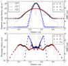 |
Fig. 1 Diffusion test: numerical (circles and squares) and analytical solutions (solid lines) at time t = 2 × 10-13 s. Bottom panel: relative error. The dotted line corresponds to the AMR levels in the simulation. |
3.2. Radiating plane
Graziani (2008) proposed an analytical multigroup test in spherical geometry. We consider a sphere of radius R and temperature Ts that is surrounded by a cold medium at temperature T0<Ts, heat capacity Cv, and spectral absorption coefficient ρκν = σν. The test consists in computing the time-dependent spectrum at a given distance r>R from the sphere centre in the absence of any hydrodynamic motion. In the case where the heat capacity tends to infinity, the gas temperature is constant, and the spectrum is the superposition of the black-body spectrum of the cold medium and the spectrum of the radiation emitted by the hot sphere. The analytical solution for the spectral energy is ![Mathematical equation: \begin{eqnarray} E_{\nu}=B(\nu,T_0)+\frac{R}{r}\left[B(\nu,T_{\mathrm{s}})-B(\nu,T_0)\right]F(\nu,r-R,t) , \end{eqnarray}](/articles/aa/full_html/2015/06/aa25971-15/aa25971-15-eq68.png) (8)where
(8)where ![Mathematical equation: \begin{eqnarray} \nonumber F(\nu,d,t)&=&\frac{{\rm e}^{-\sqrt{3} \sigma_{\nu} d}}{2} \left[\mathrm{erfc}\left(\frac12 \sqrt{\frac{3\sigma_{\nu}}{4ct}}d-\sqrt{ct\sigma_{\nu}}\right) \right.\\ &&+ \left. \mathrm{erfc}\left(\frac12 \sqrt{\frac{3\sigma_{\nu}}{4ct}}d+\sqrt{ct\sigma_{\nu}}\right) \right] . \end{eqnarray}](/articles/aa/full_html/2015/06/aa25971-15/aa25971-15-eq69.png) (9)As our grid is Cartesian, we adapted this test to a slab geometry. Instead of a radiating sphere, we consider a radiating plane. The analytical solution can then be found by setting r = R = + ∞ while keeping the distance r−R constant (Gentile 2008). We then simply have
(9)As our grid is Cartesian, we adapted this test to a slab geometry. Instead of a radiating sphere, we consider a radiating plane. The analytical solution can then be found by setting r = R = + ∞ while keeping the distance r−R constant (Gentile 2008). We then simply have ![Mathematical equation: \begin{eqnarray} E_{\nu}=B(\nu,T_0)+\left[B(\nu,T_{\mathrm{s}})-B(\nu,T_0)\right]F(\nu,r-R,t) . \end{eqnarray}](/articles/aa/full_html/2015/06/aa25971-15/aa25971-15-eq72.png) (10)In our simulation, the temperature of the hot slab was set to Ts = 1500 eV and the medium was at T0 = 50 eV. The domain size is 0.1347368 cm with the hot slab located at the left boundary. The domain was divided into 32 identical cells. We considered 60 groups logarithmically evenly spaced in the range [0.5 eV, 306 keV], a fixed timestep of Δt = 10-11 s was used, and no flux limiter (i.e. λg = 1 / 3) was applied. The gas absorption coefficient was set to
(10)In our simulation, the temperature of the hot slab was set to Ts = 1500 eV and the medium was at T0 = 50 eV. The domain size is 0.1347368 cm with the hot slab located at the left boundary. The domain was divided into 32 identical cells. We considered 60 groups logarithmically evenly spaced in the range [0.5 eV, 306 keV], a fixed timestep of Δt = 10-11 s was used, and no flux limiter (i.e. λg = 1 / 3) was applied. The gas absorption coefficient was set to  cm-1 with hνg the energy in eV of the middle of each radiative group. Figure 2 shows the spectral radiative energies obtained compared to the analytical ones at a time t = 10-10 s, sampled at a distance x = 0.04 cm (which implies that r−R = 0.04 cm in the analytical solution), which corresponds to the centre of the tenth cell. The numerical results are in excellent agreement with the analytical solution.
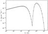 |
Fig. 2 Radiating plane test: numerical (circles) and analytical solutions at time t = 10-10 s. |
3.3. Non-equilibrium radiative transfer with picket fence model
Su & Olson (1999) developed analytical solutions for a 1D problem involving non-equilibrium radiative transfer with two radiative energy groups (see also Zhang et al. 2013). Radiative energy is injected into a small region of a uniform domain, diffuses, and heats up the gas. The two groups have different opacities, and so the radiative energies propagate at different speeds through the medium. There are several assumptions in their analytical study. The heat capacity at constant volume is assumed to be Cv = dϵ/ dT = αT3, where α is a parameter. The group integrated Planck distribution is assumed to be  (11)where aR is the radiation constant, and pg are parameters that verify the condition ∑ gpg = 1. They then define the dimensionless coordinate
  , where z is the coordinate in physical units, and
  . The absorption coefficients σg are independent of frequency, and scattering is ignored. The dimensionless time is
  (12)and the dimensionless radiative energy density and internal energy are
  (13)respectively, where T0 is a reference temperature.
The radiation source is applied for a finite period of time (0 ≤ τ<τ0) inside the region | x | <x0, and gas dynamics are neglected. The equations solved are then 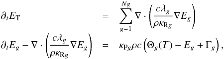 (14)where
 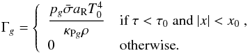 (15)Following Zhang et al. (2013), we performed case
  of Su & Olson (1999) and compared the results with their analytical solution for the radiation diffusion. In case there are two radiation groups, with p1 = p2 = 1 / 2. The absorption coefficients are chosen as σ1 = 2 / 101 cm-1 and σ2 = 200 / 101 cm-1, and the parameter α used to evaluate the heat capacity is α = 4aR. The reference temperature is set to T0 = 106 K. The radiation source parameters are x0 = 1 / 2 and τ0 = 10. To avoid spurious boundary condition effects, we used a computational domain twice the size of Zhang et al. (2013), spanning −102.4 <x< 102.4, divided into 2048 identical cells. The left and right boundary conditions were both set to periodic. The initial state of the physical variables were ρ = 1 g cm-3 and T = 1 K, and matter and radiation were in equilibrium. A fixed timestep Δτ = 0.1 was used, and no flux limiter (i.e. λg = 1 / 3) was applied. The results are shown in Fig. 3, where an excellent agreement between the numerical and analytical solutions can be seen.
3.4. Radiative shocks with non-equilibrium diffusion
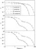 |
Fig. 3 Non-equilibrium radiative transfer test from Su & Olson (1999). Profiles from the numerical simulation of U1 (top), U2 (middle), and V (bottom) are shown for τ = 3 (solid lines) and τ = 30 (dashed lines). The results are compared to the analytical solutions of Su & Olson (1999) for τ = 3 (circles) and τ = 30 (diamonds). |
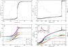 |
Fig. 4 Radiative shocks with non-equilibrium diffusion. Left column: results for the ℳ = 2 case, while the right column gives the ℳ = 5 setup. In all panels the numerical results are marked by symbols (circles and squares), the analytical solutions are represented by solid lines, and the mesh AMR level by dotted black lines. Panels a) and c): gas density as a function of distance. Panels b) and d): gas (black) and total radiative (magenta) temperatures. They also present the radiative temperatures inside the individual groups θg = (Eg/aR)1 / 4 with more colours (see legend in panel d)). |
The fourth test looks at the coupling between the fluid motion and the radiative transfer, solving the complete radiation-hydrodynamics equations (Eq. (1)). Lowrie & Edwards (2008) developed semi-analytic solutions to a 1D non-equilibrium diffusion problem involving radiative shocks of various Mach numbers ℳ. We simulated the ℳ = 2 and ℳ = 5 cases using six frequency groups. For both runs, the domain was split into two uniform regions where the hydrodynamic and radiation variables satisfy the Rankine-Hugoniot jump relations for a radiating fluid in an optically thick medium. The fluid variables inside the ghost cells at the left and right boundary conditions were kept as the initial pre- and post-shock state values throughout the simulation (imposed boundary condition). The gas has an ideal equation of state with a mean atomic weight μ = 1 and a specific heat ratio γ = 5 / 3, and the Planck and Rosseland opacities are set to ρκP = 3.93 × 10⁻⁵ cm-1 and ρκR = 0.848902 cm-1, respectively, in all frequency groups. We used the HLL Riemann solver for the hydrodynamics with a CFL factor of 0.5 and no flux-limiter for the radiation solver (i.e. λg = 1 / 3).
For the ℳ = 2 case, the initial conditions in the left (pre-shock) region are ρL = 5.45887 × 10⁻¹³ g cm-3, uL = 2.3547 × 105 cm s-1, and TL = 100 K, and in the right (post-shock) region ρR = 1.2479 × 10⁻¹² g cm-3, uR = 1.03 × 105 cm s-1, and TR = 207.757 K. The domain ranges from –1000 cm to 1000 cm. Five frequency groups were evenly (linearly) distributed between 0 and 2 × 10¹³ Hz, and the sixth group ranged from 2 × 10¹³ Hz to infinity. The domain was initially divided into 32 cells and four additional AMR levels were enabled (effective resolution of 512). The refinement criterion was based on gas density and total radiative energy gradients. The density and temperature (gas and radiation) profiles are shown in Figs. 4a,b. The numerical solutions show an excellent agreement with the semi-analytical solutions of Lowrie & Edwards (2008). The simulation data were shifted by 13.67 cm to place the density discontinuity at x = 0 for comparison with the analytical solutions; this corresponds to the shift the shock suffers as the radiative precursor develops and until the stationary state is reached.
In the ℳ = 5 case, the initial conditions are ρL = 5.45887 × 10⁻¹³ g cm-3, uL = 5.8868 × 105 cm s-1, TL = 100 K, and ρR = 1.96405 × 10⁻¹² g cm-3, uR = 1.63 × 105 cm s-1, and TR = 855.72 K. The domain ranges from –4000 cm to 4000 cm. Five frequency groups were evenly (linearly) distributed between 0 and 1014 Hz, and the sixth group ranged from 1014 Hz to infinity. The domain was initially divided into 32 cells and seven additional AMR levels were enabled (effective resolution of 4096). The refinement criterion was based on gas density, gas temperature, and total radiative energy gradients. The results in Figs 4c,d show again an excellent agreement with the semi-analytical solutions. The simulation data were this time shifted by 193.5 cm to bring the density discontinuity to x = 0.
4. Algorithm performance
We present in this section some tests to assess the scaling performance of our algorithm.
4.1. Strong and weak scaling
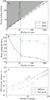 |
Fig. 5 a) Strong scaling results for the multigroup diffusion test (circles) and the ideal MHD Orszag-Tang vortex calculation (diamonds). The ideal theoretical speedup is at the boundary between the grey and white areas. The Occigen machine has 12-core processors; the 12-core region is marked by the green hatched area. b) Weak scaling efficiency for the RHD and MHD runs. c) CPU time per BiCGSTAB iteration for a 1D diffusion problem (circles) and a 1D non-stationary radiative shock (squares) as a function of the number of frequency groups Ng used. The curve for a time proportional to |
The strong and weak scaling runs were performed on the CINES Occigen3 supercomputer, which uses Intel E5-2690 (2.60 GHz) processors. We compared the scaling of our radiative transfer scheme to the native MHD scheme in RAMSES. The setups used for the RHD and MHD runs were a 2D version of the Dirac diffusion test using four frequency groups and a 2D Orszag-Tang vortex simulation (Orszag & Tang 1979), respectively. In the RHD calculation, the fluid is static and only the radiation solver was called by RAMSES, bypassing the hydrodynamic Godunov solver. Both setups used a 20482 mesh.
The strong scaling results are given in Fig. 5a. We can see that as we go beyond the 12-core limit of the Occigen processors, the speedups drop below the ideal curve (grey area) as communications begin to take longer to complete. Our radiative transfer method appears to perform slightly better than the native MHD scheme in RAMSES, as the coupling between hydrodynamics and radiation is ignored (the Godunov solver is not used in the RHD simulations). In the weak scaling RHD runs, when the size of the problem is doubled with the number of CPUs, it takes the implicit BiCGSTAB solver more iterations to converge because there is a stronger propagation of round-off errors originating from the calls to the MPI_ALLREDUCE routine when more CPUs are used. To ensure a fair comparison, we forced all simulations to execute the same number of iterations (500) for every timestep, chosen as the maximum observed number of iterations in the 1024-core run. All simulations also performed the same number of timesteps (100) of a fixed length in time (Δt = 10-17 s), and each CPU held a grid of 1282 cells. The weak MHD simulations were run for 300 timesteps, with each CPU processing a grid of 5122 cells4. The results in Fig. 5b show that the weak scaling performance of the RHD solver is below the native MHD solver. The iterative implicit solver suffers from heavy communication operations to compute residuals and scalar quantities which need to be performed at each iteration for each timestep, while the MHD solver only requires one communication operation per timestep. We believe that a weak scaling efficiency of 60% is acceptable for our purposes.
4.2. Group scaling
Our final performance test was to assess the scaling of our multigroup algorithm for a given problem when the number of frequency groups Ng is increased. The results of the simulation time divided by the total number of BiCGSTAB iterations for a 1D multigroup diffusion test performed on a single Intel Xeon E5620 (2.40 GHz) CPU core on a local HP-Z800 workstation are shown in Fig. 5c. The algorithm appears to scale with  , which is expected from the double sum over Ng in the term in the third line of Eq. (5). We carried out a second group scaling study, this time running the subcritical radiative shock test from Sect. 3.4 (although with a lower resolution; only three levels of refinement were used5), where the radiative transfer is fully coupled to the hydrodynamics. The results are given in Fig. 5c, and the behaviour is very similar to the diffusion-only solver. The radiative transfer step completely dominates over the hydrodynamic step6 in terms of computational cost, and it is thus not surprising to see the same scaling for a RHD run as for a calculation which only calls the radiation solver.
5. Application to star formation
In this final section, we apply the multigroup formalism to a simulation of the collapse of a gravitationally unstable dense cloud core, which eventually forms a protostar in its centre. The collapsing material is initially optically thin and all the energy gained from compressional heating is transported away by the escaping radiation, which causes the cloud to collapse isothermally. As the optical depth of the cloud rises, the cooling is no longer effective and the system starts heating up, taking the core collapse through its adiabatic phase. A hydrostatic body (also known as the first Larson core; Larson 1969) approximately 10 AU in size is formed and continues to accrete material from the surrounding envelope and accretion disk; this first core will eventually form a young star, after a second phase of collapse triggered by the dissociation of H2 molecules (see Masunaga & Inutsuka 2000, for instance). In this preliminary astrophysical application, however, we focus on the properties of the first Larson core for the sake of simplicity.
We adopt initial conditions similar to those in Commerçon et al. (2010), who follow Boss & Bodenheimer (1979). A magnetized uniform-density sphere of molecular gas, rotating about the z-axis with solid-body rotation, is placed in a surrounding medium a hundred times less dense. The gas and radiation temperatures are 10 K everywhere. The prestellar core mass has a mass of 1 M⊙, a radius R0 = 2500 AU, and a ratio of rotational over gravitational energy of 0.03. To favor fragmentation, we use an m = 2 azimuthal density perturbation with an amplitude of 10%. The magnetic field is initially parallel to the rotation axis. The strength of the magnetic field is expressed in terms of the mass-to-flux to critical mass-to-flux ratio μ = (M/ Φ) / (M/ Φ)c = 5 (Mouschovias & Spitzer 1976). The field strength is invariant along the z direction, and it is 100 times stronger in a cylinder of radius R0 (with the dense core in its centre) than in the surrounding medium7. We used a gas equation of state modelling a simple mixture of 73% hydrogen and 27% helium (in mass), which takes into account the effects of rotational (for H2 which is the dominant form of hydrogen for temperatures below 2000 K) and vibrational degrees of freedom. The frequency-dependent dust and gas opacities were taken from Vaytet et al. (2013a), assuming a 1% dust content. We used the ideal MHD solver of RAMSES, and the grid refinement criterion was based on the Jeans mass, ensuring the Jeans length was always sampled by a minimum of 12 cells. The coarse grid had a resolution of 323, and 11 levels of AMR were enabled, resulting in a maximum resolution of 0.15 AU at the finest level. The Minerbo flux limiter (Minerbo 1978) was used for these simulations.
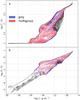 |
Fig. 6 a) Temperature as a function of density in the grey and multigroup simulations at a time t = 24 265 yr. The colour blue represents regions where the grey simulation either dominates (in terms of mass contained within the figure pixels) over the multigroup simulation, or where there is no multigroup data. Likewise, red codes for the regions of the diagram where the multigroup run prevails. The white areas indicate where both simulations yield identical results. The black contour line delineates the region where data are present. b) Same as for a) but showing the strength of the magnetic field as a function of density. |
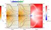 |
Fig. 7 a) Temperature map (colours) at a time t = 24 282 yr in a grey simulation of the collapse of a 1 M⊙ cloud. The data are presented as a function of radius and height over the mid-plane; the data have been averaged around the azimuthal direction. The black lines are logarithmically spaced density contours, in the range 10-16<ρ< 10-9 g cm-3 (two contours per order of magnitude). The arrows represent the velocity vector field in the r-z plane. b) Same as for a) but using 20 frequency groups. c) Map of the logarithm of the ratio of the multigroup temperature over the grey temperature. The colour red indicates where the gas temperature in the multigroup simulation is higher than for the grey run, and vice versa for blue. |
We performed two simulations; one under the grey approximation and a second using 20 frequency groups. The first and last groups spanned the frequency ranges (in Hz) [0 → 5 × 10¹⁰] and [1.3 × 10¹⁴ → ∞], respectively. The remaining 18 groups were evenly (logarithmically) distributed between 5 × 10¹⁰ and 1.3 × 10¹⁴ Hz. The results are shown in Figs. 6 and 7. The gas temperature as a function of density for all the cells in the computational domain is shown in Fig. 6a. While the two simulations show similar results overall, there are several differences we wish to point out. For relatively low densities in the range 5 × 10-17<ρ< 3 × 10-15 g cm-3, the multigroup run is hotter than the grey simulation. This is also visible in the temperature maps of Fig. 7, where the gas is hotter in the 20-group run for r> 20 AU, this being most obvious in panel c. It appears that the radiation transport from the central core to the surrounding envelope is more efficient in the multigroup case. More energy has left the core, leaving it colder than in the grey case, while more energy has been deposited in the thus warmer outer envelope. Higher temperatures are also observed in the bipolar outflow, along the vertical axis, relatively close to the first core. Kuiper et al. (2011) found that using a frequency-dependent scheme in simulations of high-mass stars could enhance radiation pressure in the polar direction compared to the grey simulations of Krumholz et al. (2009), producing much stabler outflows. This could be similar to what we are observing here; confirmation of this would require further study.
Conversely, the strength of the magnetic field does not change significantly when using a multigroup model. For densities below 10-15 g cm-3, the two runs are virtually identical (see Fig. 6b). In the ideal MHD limit, the magnetic field is not directly related to the thermal properties of the gas, and it is therefore not surprising that the multigroup formalism has little impact. However, in the future we plan to study star formation using a non-ideal description of MHD (Masson et al. 2012), where magnetic and thermal interactions are twofold. First, magnetic diffusion contributes additional gas heating from ion-neutral frictions and Joule heating. Second, the chemical properties of the gas, which strongly depend on temperature, also affect the magnetic resistivities, which govern the diffusion processes. We will investigate this in detail in a forthcoming study.
The use of multigroup RHD may not yield significantly different results in the early stages of molecular cloud collapse, but it does provide a wealth of physical information in the system. Channel maps such as the ones presented in Fig. 8 or spectral energy distributions (SEDs; Fig. 9) are directly available from the simulation data and do not require any post-processing software. The channel maps show a peak intensity around a wavelength of 100 μm, close to the synthetic observations of Commerçon et al. (2012). Interestingly, the SEDs show departures from a black-body spectrum (most obviously at the low-frequency end) close to the protostar (20 AU; Fig. 9b). We do not wish to carry out a detailed study here on the effects of multifrequency radiative transfer on the structures of protostars, we simply wish to illustrate the power of the method. We leave the detailed work on collapsing objects for a future paper, as this is first and foremost an article focused on methodology.
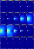 |
Fig. 8 Radiative energy density map in each frequency group. The white contours have 10 levels logarithmically spaced between the minimum and maximum values of each map. The frequencies of each group are indicated at the bottom of each map. The maps represent the same region as in Fig. 7. |
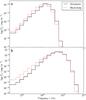 |
Fig. 9 Spectral energy distributions extracted in a cell located 2000 AU a) and 20 AU b) from the protostar. The black solid lines represent the energy inside the 20 frequency groups. They are compared to a black-body distribution (dashed red), which would have the same total energy. |
6. Conclusions and future work
We have implemented a method for multigroup flux-limited diffusion in the RAMSES AMR code for astrophysical fluid dynamics. The method is based on the time-implicit grey FLD solver of Commerçon et al. (2011b), and uses the adaptive time-stepping strategy of Commerçon et al. (2014), where each level is able to evolve with its own timestep using a subcycling procedure. The multigroup method allows the discretization of the frequency domain to any desired resolution, enabling us to take into account the frequency dependence of emission and absorption coefficients. The radiative energy density in the frequency groups are all coupled together through the matter temperature and terms reproducing Doppler shift effects when velocity gradients are present in the fluid. A consequence of this coupling is the apparition of non-symmetric terms in the matrix we have to invert in our implicit time-stepping procedure. We therefore had to abandon the original conjugate gradient algorithm of Commerçon et al. (2011b) for a bi-conjugate gradient iterative solver. A more evolved BiCGSTAB solver was preferred for its greater stability compared to a raw bi-conjugate algorithm.
The method was fully tested against standard radiation diffusion, frequency-dependent, and full radiation hydrodynamics tests. It performed extremely well in all of these tests, and its scaling performance was also found to be very satisfactory.
The multigroup formalism was finally applied to a simulation of the gravitational collapse of a dense molecular cloud core in the context of star formation. The method has revealed differences between grey and frequency-dependent simulations, but more importantly uncovered departures from a black-body radiation distribution. We also illustrated the wealth of information the method brings to astrophysical studies, with the ability to directly produce channel maps and SEDs. We will carry out a much more thorough study of the effects of multigroup radiative transfer on the structures of protostars and protoplanetary discs, as well as their observable quantities, as part of a much wider parameter space study in a forthcoming paper.
The use of a direct inversion method is not suited to the very large systems of equations that need to be solved in heavy 3D simulations.
These resolutions and number of timesteps were chosen so that both RHD and MHD simulations run for approximately the same amount of time.
This explains a smaller time per iteration for the radiative shock simulations than for the diffusion runs.
The radiation solver takes up to 90% of the computation time during one timestep.
This was chosen as an attempt to reproduce the dragging in of field lines that would have happened in the formation of the dense core (see e.g. Gillis et al. 1974), while also retaining in the simplest manner the divergence-free condition for the MHD.
Acknowledgments
This work was granted access to the CINES HPC resources Jade and Occigen under the allocations x2014-047247 and x2015-047247 made by DARI/GENCI. The research leading to these results has also received funding from the European Research Council under the European Community’s Seventh Framework Programme (FP7/2007-2013 Grant Agreement No. 247060). B.C. gratefully acknowledges support from the French ANR Retour Postdoc program (ANR-11-PDOC-0031). Finally, we acknowledge financial support from the “Programme National de Physique Stellaire” (PNPS) of CNRS/INSU, France.
References
- Bate, M. R. 2012, MNRAS, 419, 3115 [NASA ADS] [CrossRef] [Google Scholar]
- Boss, A. P., & Bodenheimer, P. 1979, ApJ, 234, 289 [NASA ADS] [CrossRef] [Google Scholar]
- Chiavassa, A., Freytag, B., Masseron, T., & Plez, B. 2011, A&A, 535, A22 [NASA ADS] [CrossRef] [EDP Sciences] [Google Scholar]
- Commerçon, B., Hennebelle, P., Audit, E., Chabrier, G., & Teyssier, R. 2010, A&A, 510, L3 [NASA ADS] [CrossRef] [EDP Sciences] [Google Scholar]
- Commerçon, B., Hennebelle, P., & Henning, T. 2011a, ApJ, 742, L9 [NASA ADS] [CrossRef] [Google Scholar]
- Commerçon, B., Teyssier, R., Audit, E., Hennebelle, P., & Chabrier, G. 2011b, A&A, 529, A35 [NASA ADS] [CrossRef] [EDP Sciences] [Google Scholar]
- Commerçon, B., Launhardt, R., Dullemond, C., & Henning, T. 2012, A&A, 545, A98 [NASA ADS] [CrossRef] [EDP Sciences] [Google Scholar]
- Commerçon, B., Debout, V., & Teyssier, R. 2014, A&A, 563, A11 [NASA ADS] [CrossRef] [EDP Sciences] [Google Scholar]
- Davis, S. W., Stone, J. M., & Jiang, Y. F. 2012, ApJS, 199, 9 [NASA ADS] [CrossRef] [Google Scholar]
- Draine, B. 2003, ARA&A, 41, 241 [NASA ADS] [CrossRef] [Google Scholar]
- Ferguson, J. W., Alexander, D. R., Allard, F., et al. 2005, ApJ, 623, 585 [NASA ADS] [CrossRef] [Google Scholar]
- Fromang, S., Hennebelle, P., & Teyssier, R. 2006, A&A, 457, 371 [NASA ADS] [CrossRef] [EDP Sciences] [Google Scholar]
- Gentile, N. 2008, in Computational Methods in Transport: Verification and Validation, ed. F. Graziani (Berlin, Heidelberg: Springer), Lect. Notes Comp. Sci. Eng., 62, 135 [Google Scholar]
- Gillis, J., Mestel, L., & Paris, R. B. 1974, Ap&SS, 27, 167 [Google Scholar]
- Graziani, F. 2008, in Computational Methods in Transport: Verification and Validation, ed. F. Graziani (Berlin, Heidelberg: Springer), Lect. Notes Comp. Sci. Eng., 62, 151 [Google Scholar]
- Krumholz, M. R., Klein, R. I., McKee, C. F., Offner, S. S. R., & Cunningham, A. J. 2009, Science, 323, 754 [NASA ADS] [CrossRef] [PubMed] [Google Scholar]
- Kuiper, R., Klahr, H., Beuther, H., & Henning, T. 2011, ApJ, 732, 20 [NASA ADS] [CrossRef] [Google Scholar]
- Larson, R. B. 1969, MNRAS, 145, 271 [NASA ADS] [CrossRef] [Google Scholar]
- Levermore, C. D., & Pomraning, G. C. 1981, ApJ, 248, 321 [NASA ADS] [CrossRef] [Google Scholar]
- Li, A., & Draine, B. T. 2001, ApJ, 554, 778 [Google Scholar]
- Lowrie, R. B., & Edwards, J. D. 2008, Shock Waves, 18, 129 [NASA ADS] [CrossRef] [Google Scholar]
- Masson, J., Teyssier, R., Mulet-Marquis, C., Hennebelle, P., & Chabrier, G. 2012, ApJS, 201, 24 [NASA ADS] [CrossRef] [Google Scholar]
- Masunaga, H., & Inutsuka, S. 2000, ApJ, 531, 350 [NASA ADS] [CrossRef] [Google Scholar]
- Masunaga, H., Miyama, S. M., & Inutsuka, S.-I. 1998, ApJ, 495, 346 [Google Scholar]
- Mezzacappa, A., Calder, A. C., Bruenn, S. W., et al. 1998, ApJ, 495, 911 [NASA ADS] [CrossRef] [Google Scholar]
- Minerbo, G. N. 1978, J. Quant. Spec. Radiat. Transf., 20, 541 [NASA ADS] [CrossRef] [Google Scholar]
- Mouschovias, T. C., & Spitzer, Jr., L. 1976, ApJ, 210, 326 [NASA ADS] [CrossRef] [Google Scholar]
- Orszag, S. A., & Tang, C.-M. 1979, J. Fluid Mech., 90, 129 [NASA ADS] [CrossRef] [Google Scholar]
- Ossenkopf, V., & Henning, T. 1994, A&A, 291, 943 [NASA ADS] [Google Scholar]
- Semenov, D., Henning, T., Helling, C., Ilgner, M., & Sedlmayr, E. 2003, A&A, 410, 611 [NASA ADS] [CrossRef] [EDP Sciences] [Google Scholar]
- Shestakov, A., & Offner, S. 2008, J. Comput. Phys., 227, 2154 [NASA ADS] [CrossRef] [Google Scholar]
- Su, B., & Olson, G. 1999, J. Quant. Spec. Radiat. Transf., 62, 279 [NASA ADS] [CrossRef] [Google Scholar]
- Teyssier, R. 2002, A&A, 385, 337 [NASA ADS] [CrossRef] [EDP Sciences] [Google Scholar]
- Tomida, K., Tomisaka, K., Matsumoto, T., et al. 2013, ApJ, 763, 6 [NASA ADS] [CrossRef] [Google Scholar]
- van der Holst, B., Toth, G., Sokolov, I. V., et al. 2011, ApJS, 194, 23 [NASA ADS] [CrossRef] [Google Scholar]
- van der Vorst, H. A. 1992, SIAM J. Scientific and Statistical Computing, 13, 631 [Google Scholar]
- Vaytet, N., Audit, E., Dubroca, B., & Delahaye, F. 2011, J. Quant. Spectr. Rad. Transf., 112, 1323 [NASA ADS] [CrossRef] [Google Scholar]
- Vaytet, N., Audit, E., Chabrier, G., Commerçon, B., & Masson, J. 2012, A&A, 543, A60 [NASA ADS] [CrossRef] [EDP Sciences] [Google Scholar]
- Vaytet, N., Chabrier, G., Audit, E., et al. 2013a, A&A, 557, A90 [NASA ADS] [CrossRef] [EDP Sciences] [Google Scholar]
- Vaytet, N., González, M., Audit, E., & Chabrier, G. 2013b, J. Quant. Spectr. Rad. Transf., 125, 105 [Google Scholar]
- Williams, R. B. 2005, Ph.D. Thesis, Massachusetts Institute of Technology, Dept. of Nuclear Engineering [Google Scholar]
- Zhang, W., Howell, L., Almgren, A., et al. 2013, ApJS, 204, 7 [NASA ADS] [CrossRef] [Google Scholar]
All Figures
|
Fig. 1 Diffusion test: numerical (circles and squares) and analytical solutions (solid lines) at time t = 2 × 10-13 s. Bottom panel: relative error. The dotted line corresponds to the AMR levels in the simulation. |
| In the text | |
|
Fig. 2 Radiating plane test: numerical (circles) and analytical solutions at time t = 10-10 s. |
| In the text | |
|
Fig. 3 Non-equilibrium radiative transfer test from Su & Olson (1999). Profiles from the numerical simulation of U1 (top), U2 (middle), and V (bottom) are shown for τ = 3 (solid lines) and τ = 30 (dashed lines). The results are compared to the analytical solutions of Su & Olson (1999) for τ = 3 (circles) and τ = 30 (diamonds). |
| In the text | |
|
Fig. 4 Radiative shocks with non-equilibrium diffusion. Left column: results for the ℳ = 2 case, while the right column gives the ℳ = 5 setup. In all panels the numerical results are marked by symbols (circles and squares), the analytical solutions are represented by solid lines, and the mesh AMR level by dotted black lines. Panels a) and c): gas density as a function of distance. Panels b) and d): gas (black) and total radiative (magenta) temperatures. They also present the radiative temperatures inside the individual groups θg = (Eg/aR)1 / 4 with more colours (see legend in panel d)). |
| In the text | |
|
Fig. 5 a) Strong scaling results for the multigroup diffusion test (circles) and the ideal MHD Orszag-Tang vortex calculation (diamonds). The ideal theoretical speedup is at the boundary between the grey and white areas. The Occigen machine has 12-core processors; the 12-core region is marked by the green hatched area. b) Weak scaling efficiency for the RHD and MHD runs. c) CPU time per BiCGSTAB iteration for a 1D diffusion problem (circles) and a 1D non-stationary radiative shock (squares) as a function of the number of frequency groups Ng used. The curve for a time proportional to |
| In the text | |
|
Fig. 6 a) Temperature as a function of density in the grey and multigroup simulations at a time t = 24 265 yr. The colour blue represents regions where the grey simulation either dominates (in terms of mass contained within the figure pixels) over the multigroup simulation, or where there is no multigroup data. Likewise, red codes for the regions of the diagram where the multigroup run prevails. The white areas indicate where both simulations yield identical results. The black contour line delineates the region where data are present. b) Same as for a) but showing the strength of the magnetic field as a function of density. |
| In the text | |
|
Fig. 7 a) Temperature map (colours) at a time t = 24 282 yr in a grey simulation of the collapse of a 1 M⊙ cloud. The data are presented as a function of radius and height over the mid-plane; the data have been averaged around the azimuthal direction. The black lines are logarithmically spaced density contours, in the range 10-16<ρ< 10-9 g cm-3 (two contours per order of magnitude). The arrows represent the velocity vector field in the r-z plane. b) Same as for a) but using 20 frequency groups. c) Map of the logarithm of the ratio of the multigroup temperature over the grey temperature. The colour red indicates where the gas temperature in the multigroup simulation is higher than for the grey run, and vice versa for blue. |
| In the text | |
|
Fig. 8 Radiative energy density map in each frequency group. The white contours have 10 levels logarithmically spaced between the minimum and maximum values of each map. The frequencies of each group are indicated at the bottom of each map. The maps represent the same region as in Fig. 7. |
| In the text | |
|
Fig. 9 Spectral energy distributions extracted in a cell located 2000 AU a) and 20 AU b) from the protostar. The black solid lines represent the energy inside the 20 frequency groups. They are compared to a black-body distribution (dashed red), which would have the same total energy. |
| In the text | |
Current usage metrics show cumulative count of Article Views (full-text article views including HTML views, PDF and ePub downloads, according to the available data) and Abstracts Views on Vision4Press platform.
Data correspond to usage on the plateform after 2015. The current usage metrics is available 48-96 hours after online publication and is updated daily on week days.
Initial download of the metrics may take a while.