© ESO, 2015

1. Introduction

The exoplanet class of hot Jupiters consists of massive gaseous planets (of mass ~1–10 M_J, where the subscript “J” denotes the planet Jupiter) that orbit their host stars on close-in trajectories (semi-major axis of ≲0.1 AU, corresponding to an orbital period of a few days). Among other exoplanets, the size and location of hot Jupiters favors both their discovery and the collection of detailed data. The two leading and complementary detection techniques, radial velocity and transit observations, have resulted in a wealth of information regarding their orbital characteristics, such as obliquity and eccentricity (e.g., Fabrycky & Winn 2009), as well as their physical properties, such as surface temperature and atmospheric composition (e.g., Bean et al. 2013). The study of the phenomenology of hot Jupiters also provides valuable input to research on the physical conditions and processes in smaller, harder-to-probe, Neptune- and Earth-like bodies (see, e.g., Seager 2011 for a recent reference on exoplanets).

Hot-Jupiter atmospheres are believed to be heated by photoionizing extreme-ultraviolet (EUV) stellar irradiation (e.g., Burrows et al. 2000; but see also Owen & Jackson 2012 as well as Buzasi 2013 and Lanza 2013, who proposed, respectively, X-rays for very young stars and magnetic reconnection for very close-in planets). The energy input could be large enough to induce an evaporative mass loss at a rate of ~10¹⁰−10¹² g s^-1. Such outflows have been inferred in a couple of systems (HD 189733b and HD 209458b) in which detailed observations have been carried out (e.g., Vidal-Madjar et al. 2004; Ehrenreich et al. 2008; Lecavelier des Etangs et al. 2010, 2012; Bourrier et al. 2013; although see Ben-Jaffel 2007, 2008 for a different interpretation of the data). The theory of evaporative planetary outflows has been developed in a number of papers, taking into account the thermal and ionization structure of the irradiated planetary atmosphere as well as tidal and magnetic effects (e.g., Lecavelier des Etangs et al. 2004; Yelle 2004, 2006; Tian et al. 2005; García Muñoz 2007; Murray-Clay et al. 2009; Adams 2011; Trammell et al. 2011, 2014; Koskinen et al. 2013; Owen & Adams 2014, and references therein).

The host stars of close-in planets typically drive magnetized stellar winds that are accelerated to speeds of a few hundred km s^-1. The properties of these winds change as the star evolves, from strong and often collimated outflows in young stars (e.g., Matt & Pudritz 2008; Matt et al. 2012b) to weak and more isotropic winds during the main-sequence phase (e.g., Matt et al. 2012a; Cohen & Drake 2014, and references therein). The magnetized plasma that is driven out in these winds constitutes the medium into which the evaporative outflows from close-in exoplanets expand.

A close-in planet and its host star could thus interact through their respective outflows and/or magnetic fields. In either case, the interaction could have a potentially observable signature. For example, it has been suggested that there might be a detectable bow shock formed by the supersonic stellar wind in front of the planet (e.g., Vidotto et al. 2010, 2011a,b, 2014; Llama et al. 2011, 2013; Ben-Jaffel & Ballester 2013), or an observable cometary-type tail associated with the swept-up planetary wind that trails the planet in its orbit (e.g., Schneider et al. 1998; Mura et al. 2011; Kulow et al. 2014). According to these proposals, a bow shock could potentially contribute to the absorption of stellar radiation before an ingress of a transiting hot Jupiter, whereas a tail might contribute after an egress. It has also been proposed that the interaction with the stellar magnetosphere might lead to phased hot spots on the stellar surface or to flaring activity (Shkolnik et al. 2003, 2004, 2005, 2008; Walker et al. 2008; Lanza 2008, 2009; Cohen et al. 2009; Pillitteri et al. 2010, 2011, 2014, 2015), and that the planetary magnetic field could be affected in both its topology and its strength (e.g., Laine et al. 2008; Cohen et al. 2011b, 2014; Strugarek et al. 2014). Cohen et al. (2010) have suggested that the interaction with a magnetized hot Jupiter could lead to a reduction in the mass loss rate, and even more strongly in the angular momentum loss rate, from the host star.

In this paper we perform 3D magnetohydrodynamic (MHD) simulations that aim to address the following questions:

• 1.

  How can one classify the different types of star–planetinteractions that arise when a hot Jupiter orbits its host star?

• 2.

  What are the dynamical features that develop in each case, and what are their expected observational signatures?

• 3.

  What is the impact of this interaction on the planetary and stellar outflows?

We classify such interactions by studying the evolution of a grid of numerical models. In particular, we investigate whether it is the planetary magnetosphere or the planetary outflow that intercepts the stellar plasma, whether the stellar outflow terminates in a bow shock, the circumstances for forming a stable tail along the planet’s orbit, and the conditions under which accretion streams of planetary material reach the stellar surface. We carry out a parametric study and present the criteria that can be used to classify a system’s morphology and dynamics based on its physical parameters. We also consider some general properties of the interaction regions that bear on their potential detectability.

Previous work by Cohen et al. (2009, 2011a) has identified and described some of the physical processes that may take place in a system consisting of a magnetized star and a magnetized hot Jupiter. These studies were, however, focused on the interpretation of two specific systems. In addition, the planetary outflows were not explicitly included; they developed based on the boundary conditions applied on the surface of the planet. In contrast, we perform a systematic study to classify the types of star–planet interactions, incorporating consistent planetary winds that are based on detailed models.

The paper is structured as follows. Section 2 explains the methodology and presents the numerical models. Section 3 reports the results of the simulations and describes the dynamics. Section 4 classifies the types of interaction and considers some of their potential observational manifestations. Finally, Sect. 5 summarizes the conclusions of this work.

2. Numerical modeling

As discussed in Murray-Clay et al. (2009, see also Tian et al. 2005; García Muñoz 2007, evaporative hot-Jupiter outflows need to be modeled as a fluid (using a hydrodynamic or an MHD formulation) rather than as a collection of individual particles that undergo Jeans escape because the plasma typically remains collisional beyond the flow’s critical point. Murray-Clay et al. (2009) considered an unmagnetized outflow from a hot Jupiter exposed to a UV flux near the low end of the range of values that we model (see Sect. 2.6), and evaluated the collisional mean free path ℓ_pp = 1 / (n_Hσ_pp) to proton–proton collisions in a hydrogen plasma of density n_H and temperature T ≈ 10⁴K (for which the relevant cross section is σ_pp ≈ 10^-13 [T/ 10⁴ K] ^-2 cm²). They inferred a value (≃10⁷cm) that is ~10⁴ smaller than the density scale height at the sonic point (which lies at a distance of ~5 planetary radii from the center of the planet). The large value of this ratio indicates that the collisional approximation should be applicable to this problem over a wide range of circumstances. Similarly, our simple stellar-wind model (Sect. 2.8) is also adequately modeled within the hydrodynamic framework (e.g., Parker 1960). The fact that both the planetary and the stellar outflows are likely magnetized sharpens these conclusions: for typical parameters, the proton Larmor radius ℓ_L = c_sm_pc/ (eB) (where c_s is the speed of sound, m_p is the proton mass, c is the speed of light, e is the electron charge, and B is the magnetic field amplitude) is ~10² (c_s/ 10 km s^-1)(B / 1 G)^-1cm – much smaller than ℓ_pp. Given that the region where the planetary and stellar outflows interact is located at a distance from the source of each of these winds that is comparable to the distance of its respective critical surface, an MHD treatment of this interaction should be amply justified.

A numerical simulation that encompasses both the star and the planet needs to adequately resolve the sizes of both objects. For the case of a hot Jupiter orbiting a solar-type host, the characteristic length scales of the planet and the star differ by roughly an order of magnitude. Since 3D numerical simulations are computationally demanding, the best strategy to model the star–planet interaction is to adopt multiple levels of refinement. One approach is to configure an adaptive mesh that follows the orbit of the planet and provides high resolution for its interior and environment. Another is to set up a static, multiply refined grid and combine it properly with a corotating frame of reference, so that the location of the planet stays fixed in the highly resolved region. Here we adopt the latter approach, which also simplifies the treatment of the interior of the planet. In general, a static, multiply refined grid is also appropriate for inclined orbits, as long as they are circular.

In the following, we denote the star with “∗” and the planet with “°”. The simulations are performed in Cartesian coordinates (x,y,z), but for convenience we also use the notation of spherical coordinates (R,θ,φ). The planet is assumed to orbit in the x-y plane, or, equivalently, at θ = π/ 2. The center of the star is placed at the origin, (x_∗,y_∗,z_∗) = (0, 0, 0), whereas the center of the planet at (x_°,y_°,z_°) = (x_°, 0, 0). For the initialization we use an extra set of coordinate systems denoted with primes, (x′,y′,z′) and (R′,θ′,φ′), with their origins placed at (x_°,y_°,z_°) (i.e., centered on the planet). At each spatial point (x,y,z) we first calculate (x′,y′,z′) = (x−x_°,y,z) and then perform a coordinate transformation to obtain (R′,θ′,φ′). In order to keep the center of the planet fixed, we adopt a corotating frame with Ω_fr = Ω_orb, where Ω_fr = Ω_frẑ is the angular velocity of the frame and ${\mathrm{\Omega }}_{\mathrm{orb}}\mathrm{=}\mathrm{(}\mathit{G}{\mathit{M}}_{\mathrm{\ast }}\mathit{/}{\mathit{x}}_{\mathrm{◦}}^{\mathrm{3}}{\mathrm{)}}^{\mathrm{1}\mathit{/}\mathrm{2}}$ is the Keplerian angular speed of the planet (with M_∗ being the mass of the star and G the gravitational constant). Since M_∗ ≫ M_° (where M_° is the mass of the planet), we assume that M_∗ + M_° ≃ M_∗ and hence that the origin of the coordinate system is effectively located at the center of mass.

2.1. The MHD equations

The ideal MHD equations in a frame that corotates with the planet are:

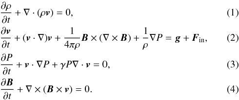$\begin{array}{ccc}& & \\ & & \\ & & \\ & & \frac{\mathit{\partial }{B}}{\mathit{\partial t}}\mathrm{+}\mathrm{\nabla }\mathrm{\times }\mathrm{(}{B}\mathrm{\times }{v}\mathrm{)}\mathrm{=}\mathrm{0.}\end{array}$The variables ρ, P, v, and B denote the density, pressure, velocity, and magnetic field, respectively, and γ is the polytropic index. The magnetic field is required to obey the solenoidal condition ∇·B = 0. Since we consider the nonrelativistic regime, ρ, P, and B have the same values in the corotating frame and in the lab (star’s center of mass) frame. The velocity in the lab frame is obtained from the expression . The vector g = g_∗ + g_° is the gravitational acceleration, and the inertial force that appears in the corotating frame, F_in = F_centr + F_cor, has centrifugal ${{F}}_{\mathrm{centr}}\mathrm{=}\mathrm{-}[{{\Omega }}_{\mathrm{fr}}\mathrm{\times }\mathrm{(}{{\Omega }}_{\mathrm{fr}}\mathrm{\times }{R}\mathrm{)}]\mathrm{=}{\mathrm{\Omega }}_{\mathrm{fr}}^{\mathrm{2}}\mathrm{(}\mathit{x}\mathit{x̂}\mathrm{+}\mathit{y}\mathit{ŷ}\mathrm{)}$(5)and Coriolis ${{F}}_{\mathrm{cor}}\mathrm{=}\mathrm{-}\mathrm{2}\mathrm{(}{{\Omega }}_{\mathrm{fr}}\mathrm{\times }{v}\mathrm{)}\mathrm{=}\mathrm{2}{\mathrm{\Omega }}_{\mathrm{fr}}\mathrm{(}{\mathit{v}}_{\mathit{y}}\mathit{x̂}\mathrm{-}{\mathit{v}}_{\mathit{x}}\mathit{ŷ}\mathrm{)}$(6)components.

The temperature at the base of an EUV-induced hot-Jupiter outflow is found to be ~10⁴ K (e.g., Murray-Clay et al. 2009): this value reflects the balance between photoionization heating and collisionally excited radiative cooling (e.g., Spitzer 1978). Furthermore, in cases where the stellar UV flux is sufficiently high, radiative cooling continues to roughly balance the photoionization heating as the wind moves away from the surface, with the result that the temperature changes little along the flow (e.g., Murray-Clay et al. 2009). The isothermal approximation was also found to apply to the inner regions of the solar wind (e.g., Cranmer et al. 2007), and has thus been adopted in previous simulations of both stellar (e.g., Matt & Pudritz 2008) and planetary (e.g., Trammell et al. 2014) outflows. Based on these considerations, we model both the stellar and the planetary outflows in our simulations as being nearly isothermal throughout, characterizing them by a polytropic index γ = 1.05 as in the fiducial model of Matt & Pudritz (2008). This approach enables us to simulate the dynamics of these winds without having to deal with the intricacies of a detailed calculation of the thermal structure of the outflow. As we show in Sect. 2.8, the adopted framework can be made to yield density and velocity profiles for the planetary wind that are compatible with the results obtained by employing the more elaborate (albeit nonmagnetic) 1D model of Murray-Clay et al. (2009), which incorporates photoionization heating and radiative as well as adiabatic cooling. Koskinen et al. (2013) – who adopted a more detailed modeling approach that included, among other factors, a consideration of the full spectrum of ionizing photons (rather than just a single representative frequency) – found quantitative differences from the Murray-Clay et al. (2009) findings (such as a slower increase of the ionization fraction with distance from the planet’s surface; see also Trammell et al. 2011), but their results remain qualitatively similar to those of Murray-Clay et al. (2009). We therefore consider the adopted approximation to be justified for the present study, especially because the classification criteria presented in Sect. 4 do not depend on the details of the wind models.

We further assume, for simplicity, that the plasma consists of pure atomic hydrogen, and that it is fully ionized, so that the temperature is given by T = Pm_p/ 2ρk_B (where the factor 1 / 2 represents the mean molecular weight, and k_B is the Boltzmann constant). The strong ionization and near-isothermality assumptions for the planetary wind are consistent with the “high UV flux” case (corresponding to a young host star; e.g., Ribas et al. 2005) presented in Murray-Clay et al. (2009). By contrast, in the “low UV flux” case considered by these authors (corresponding to a solar-analog host), the wind temperature drops with distance from the stellar surface on account of adiabatic cooling. To mimic this case, we also consider models with a characteristic temperature that is lower than 10⁴ K.

At locations where the magnetized stellar wind interacts with the planetary outflow or magnetosphere, field-line reconnection may potentially take place. This process can be realized in the simulations – even though resistivity is not explicitly included in the formulation – because numerical diffusion allows the magnetic field to reconnect in the presence of strong current sheets. We note, however, that the model setup adopted in this paper represents the star and the planet as aligned magnetic dipoles, a configuration that does not give rise to X-point structures and is therefore not prone to reconnection.

2.2. Stellar and planetary parameters

Table 1 lists the basic model parameters that characterize the host star and the Jupiter-like close-in planet. The masses (M_∗, M_°) appear in the expressions for the gravitational field outside each of the bodies, whereas the radii (R_∗, R_°) define the spheres within which an internal boundary is applied. The temperatures correspond to the values at the base of the respective outflows (the stellar corona and the UV absorption layer in the outer planetary atmosphere). The value of the density of the stellar outflow, ρ_∗, is chosen so that the mass-loss rate be comparable to that of the solar wind (a few times 10^-14M_⊙ yr^-1), an approach adopted from Matt & Pudritz (2008). For the planet, the base density value is determined from the requirement that the simulated wind match high-resolution 1D numerical simulations that include the relevant heating and cooling processes (see Sect. 2.8). Thus, ρ_° should not be regarded as the actual density at optical depth τ ~ 1 (the physical base of the outflow) but rather as a numerically motivated value that gives the appropriate wind profile. The initial magnetic fields of the star and the planet are assumed to be dipolar, with equatorial surface values equal to B_∗ and B_°, respectively.

The escape speed from the stellar surface is given by v_{esc ∗} = (2GM_∗/R_∗)^{1 / 2}, whereas the sound speed at the base of the stellar wind is c_{s ∗} = (γP_∗/ρ_∗)^{1 / 2}. A useful model parameter for determining the properties of the wind is λ_∗ ≡ (1 / 2)(v_{esc ∗}/c_{s ∗})². Another important nondimensional variable is the ratio of the thermal and magnetic pressures at the stellar surface, β_∗ ≡ P_∗/ (B_∗/ 8π) (the stellar plasma beta), which characterizes the dynamical significance of the magnetic field¹. The third relevant parameter for characterizing the outflow is ϵ_∗ ≡ (Ω_∗R_∗/c_{s ∗})², which measures the effect of surface rotation. Corresponding expressions for v_{esc °}, c_{s °}, λ_°, β_°, and ϵ_° are used for the planet.

The stellar UV flux, F_UV, is a critical quantity because it determines the energy input and hence the strength of the planetary wind. Finally, Table 1 gives the rotational periods of the star () and the planet () as well as the orbital characteristics, R_orb = x_°, , and v_orb = (GM_∗/R_orb)^{1 / 2}. The host star is taken to rotate at 1% of the breakup angular speed (as compared to 0.4% of $\mathrm{(}\mathit{G}{\mathit{M}}_{\mathrm{\ast }}\mathit{/}{\mathit{R}}_{\mathrm{\ast }}^{\mathrm{3}}{\mathrm{)}}^{\mathrm{1}\mathit{/}\mathrm{2}}$ for the present Sun), whereas the planet is assumed to be tidally locked (i.e., Ω_° = Ω_orb), which is a reasonable approximation for a close-in planet that interacts tidally with its host star (e.g., Matsumura et al. 2010). Our model planets thus rotate at ~3−26% of breakup.

2.3. Stellar and planetary winds

We base the numerical treatment of the two outflows on the simplified approach of Matt & Balick (2004). In brief, we initialize dipolar magnetospheres (force-free by definition) and keep fixed at each surface the physical quantities that drive the flow. The temporal evolution of such configurations opens up the magnetospheres and leads to steady-state winds (see Matt & Pudritz 2008). Although this method does not require the winds to be specified explicitly, we have opted to initialize a simple form of outflow to ensure that the starting wind profiles are in agreement with detailed, self-consistent models in the literature. We emphasize that, because of the transonic nature of these flows, the final steady state does not depend on the initial configurations, but only on the boundary conditions that are imposed at the surfaces of the two objects. However, in low-resolution simulations that do not include all the relevant physics, simple assumptions about the density and temperature at the boundary might not give correct results. Therefore, we use the profiles of detailed outflow models as a guide in order to set up the appropriate boundary conditions. This procedure is particularly useful for capturing the correct mass loss rate of the planet, as described in more detail in Sect. 2.8.

We initialize the velocity field of each outflow at time t = 0 as an isotropic, isothermal Parker wind (Parker 1958). In particular, the velocity profile for the stellar outflow, ${\mathit{v}}_{\mathrm{w}\hspace{0.17em}\mathrm{\ast }}^{\mathrm{init}}\mathrm{\left(}\mathit{R}\mathrm{\right)}$, is obtained by solving numerically the equation ${\mathit{\psi }}_{\mathrm{\ast }}\mathrm{-}\ln {\mathit{\psi }}_{\mathrm{\ast }}\mathrm{=}\mathrm{-}\mathrm{3}\mathrm{-}\mathrm{4}\ln \left(\frac{{\mathit{\lambda }}_{\mathrm{\ast }}}{\mathrm{2}}\right)\mathrm{+}\ln {\mathit{\xi }}_{\mathrm{\ast }}\mathrm{+}\mathrm{2}\frac{{\mathit{\lambda }}_{\mathrm{\ast }}}{{\mathit{\xi }}_{\mathrm{\ast }}}\mathit{,}$(7)where ${\mathit{\psi }}_{\mathrm{\ast }}\mathrm{\left(}\mathit{R}\mathrm{\right)}\mathrm{\equiv }\mathrm{(}{\mathit{v}}_{\mathrm{w}\hspace{0.17em}\mathrm{\ast }}^{\mathrm{init}}\mathit{/}{\mathit{c}}_{\mathrm{s}\hspace{0.17em}\mathrm{\ast }}{\mathrm{)}}^{\mathrm{2}}$, ξ_∗(R) ≡ R/R_∗, and λ_∗ is defined in Sect. 2.2. In this equation we take the speed of sound to be strictly isothermal, i.e., c_s = (2k_BT/m_p)^{1 / 2} (corresponding to a polytropic index that is exactly 1). Since the star is assumed to be rotating, we make the approximation that the initial wind is rotating rigidly with it. This is a minor contribution to the outflow velocity because Ω_∗ is an order of magnitude smaller than Ω_fr (and, in any case, the flow self-consistently assumes the correct values of v_φ as the simulation evolves). The Cartesian components of the initial stellar outflow velocity are then given by the sum of the wind, rotation, and frame speeds:

$\begin{array}{ccc}& & {\mathit{v}}_{\mathit{x}\hspace{0.17em}\mathrm{\ast }}^{\mathrm{init}}\mathrm{\left(}\mathit{x,y,z}\mathrm{\right)}\mathrm{=}\sin \mathit{\theta }\mathrm{[}\cos \mathit{\phi }\hspace{0.17em}{\mathit{v}}_{\mathrm{w}\hspace{0.17em}\mathrm{\ast }}^{\mathrm{init}}\mathrm{\left(}\mathit{R}\mathrm{\right)}\mathrm{+}\sin \mathit{\phi }\hspace{0.17em}\mathit{R}\mathrm{(}{\mathrm{\Omega }}_{\mathrm{fr}}\mathrm{+}{\mathrm{\Omega }}_{\mathrm{\ast }}{\mathrm{)}}^{\mathrm{]}}\mathit{,}\\ & & {\mathit{v}}_{\mathit{y}\hspace{0.17em}\mathrm{\ast }}^{\mathrm{init}}\mathrm{\left(}\mathit{x,y,z}\mathrm{\right)}\mathrm{=}\sin \mathit{\theta }\mathrm{[}\sin \mathit{\phi }\hspace{0.17em}{\mathit{v}}_{\mathrm{w}\hspace{0.17em}\mathrm{\ast }}^{\mathrm{init}}\mathrm{\left(}\mathit{R}\mathrm{\right)}\mathrm{-}\cos \mathit{\phi }\hspace{0.17em}\mathit{R}\mathrm{(}{\mathrm{\Omega }}_{\mathrm{fr}}\mathrm{+}{\mathrm{\Omega }}_{\mathrm{\ast }}{\mathrm{)}}^{\mathrm{]}}\mathit{,}\\ & & {\mathit{v}}_{\mathit{z}\hspace{0.17em}\mathrm{\ast }}^{\mathrm{init}}\mathrm{\left(}\mathit{x,y,z}\mathrm{\right)}\mathrm{=}\cos \mathit{\theta }\hspace{0.17em}{\mathit{v}}_{\mathrm{w}\hspace{0.17em}\mathrm{\ast }}^{\mathrm{init}}\mathrm{\left(}\mathit{R}\mathrm{\right)}\mathit{.}\end{array}$To derive the corresponding expressions for the planetary outflow, we first calculate ${\mathit{v}}_{\mathrm{w}\hspace{0.17em}\mathrm{◦}}^{\mathrm{init}}\mathrm{\left(}{\mathit{R}}^{\mathrm{\prime }}\mathrm{\right)}$ from Eq. (7), using ψ_°(R′), λ_°, and ξ_°(R′) ≡ R′/R_°. We then add the planet’s orbital velocity, v_orb = R_orbΩ_orbŷ, as well as the frame and planetary-rotation velocities (using the rigid-body assumption), to obtain

$\begin{array}{ccc}& & {\mathit{v}}_{\mathit{x}\hspace{0.17em}\mathrm{◦}}^{\mathrm{init}}\mathrm{\left(}\mathit{x,y,z}\mathrm{\right)}\mathrm{=}\sin {\mathit{\theta }}^{\mathrm{\prime }}[\cos {\mathit{\phi }}^{\mathrm{\prime }}{\mathit{v}}_{\mathrm{w}\hspace{0.17em}\mathrm{◦}}^{\mathrm{init}}\mathrm{\left(}{\mathit{R}}^{\mathrm{\prime }}\mathrm{\right)}\\ & & \mathrm{+}\sin \mathit{\phi }\hspace{0.17em}\mathit{R}{\mathrm{\Omega }}_{\mathrm{fr}}\mathrm{-}\sin {\mathit{\phi }}^{\mathrm{\prime }}{\mathit{R}}^{\mathrm{\prime }}{\mathrm{\Omega }}_{\mathrm{◦}}]\mathit{,}\\ & & {\mathit{v}}_{\mathit{y}\hspace{0.17em}\mathrm{◦}}^{\mathrm{init}}\mathrm{\left(}\mathit{x,y,z}\mathrm{\right)}\mathrm{=}\sin {\mathit{\theta }}^{\mathrm{\prime }}[\sin {\mathit{\phi }}^{\mathrm{\prime }}{\mathit{v}}_{\mathrm{w}\hspace{0.17em}\mathrm{◦}}^{\mathrm{init}}\mathrm{\left(}{\mathit{R}}^{\mathrm{\prime }}\mathrm{\right)}\\ & & \mathrm{-}\cos \mathit{\phi }\hspace{0.17em}\mathit{R}{\mathrm{\Omega }}_{\mathrm{fr}}\mathrm{+}{\mathit{R}}_{\mathrm{orb}}{\mathrm{\Omega }}_{\mathrm{orb}}\mathrm{+}\cos {\mathit{\phi }}^{\mathrm{\prime }}{\mathit{R}}^{\mathrm{\prime }}{\mathrm{\Omega }}_{\mathrm{◦}}]\mathit{,}\\ & & {\mathit{v}}_{\mathit{z}\hspace{0.17em}\mathrm{◦}}^{\mathrm{init}}\mathrm{\left(}\mathit{x,y,z}\mathrm{\right)}\mathrm{=}\cos {\mathit{\theta }}^{\mathrm{\prime }}{\mathit{v}}_{\mathrm{w}\hspace{0.17em}\mathrm{◦}}^{\mathrm{init}}\mathrm{\left(}{\mathit{R}}^{\mathrm{\prime }}\mathrm{\right)}\mathit{,}\end{array}$where R′, θ′, and φ′ are functions of (x,y,z), as explained at the beginning of this section. For simplicity, we have assumed that the initial planetary wind orbits and spins rigidly with the planet, an approximation that is appropriate only close to the surface. We note that, for a tidally locked planet, the orbital velocity cancels out with the frame and planetary rotation velocities, and the planet stays fixed at the location (x_°,y_°,z_°). For example, the sum of the y components of these three terms at a distance x along the line that connects the centers of the star and the planet is −xΩ_fr + x_°Ω_orb + x′Ω_° = 0. Under these assumptions, given that we are working in the corotating frame, we could have just as well initialized the velocity by using only the thermal (Parker) wind, with no extra terms.

To obtain the pressure profile of the stellar wind, we solve analytically the hydrodynamic radial momentum equation, 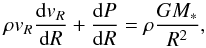$\mathit{\rho }{\mathit{v}}_{\mathit{R}}\frac{\mathrm{d}{\mathit{v}}_{\mathit{R}}}{\mathrm{d}\mathit{R}}\mathrm{+}\frac{\mathrm{d}\mathit{P}}{\mathrm{d}\mathit{R}}\mathrm{=}\mathit{\rho }\frac{\mathit{G}{\mathit{M}}_{\mathrm{\ast }}}{{\mathit{R}}^{\mathrm{2}}}\mathit{,}$(14)which gives ${\mathit{P}}_{\mathrm{\ast }}^{\mathrm{init}}\mathrm{\left(}\mathit{x,y,z}\mathrm{\right)}\mathrm{=}{\mathit{P}}_{\mathrm{\ast }}\exp \left[{\mathit{\lambda }}_{\mathrm{\ast }}\left(\frac{{\mathit{R}}_{\mathrm{\ast }}}{\mathit{R}}\mathrm{-}\mathrm{1}\right)\mathrm{-}\frac{\mathrm{1}}{\mathrm{2}}{\left(\frac{{\mathit{v}}_{\mathrm{w}\hspace{0.17em}\mathrm{\ast }}^{\mathrm{init}}}{{\mathit{c}}_{\mathrm{s}\hspace{0.17em}\mathrm{\ast }}}\right)}^{\mathrm{2}}\right]\mathit{.}$(15)The density is then found using the isothermal-plasma assumption: ${\mathit{\rho }}_{\mathrm{\ast }}^{\mathrm{init}}\mathrm{\left(}\mathit{x,y,z}\mathrm{\right)}\mathrm{=}\frac{{\mathit{\rho }}_{\mathrm{\ast }}}{{\mathit{P}}_{\mathrm{\ast }}}{\mathit{P}}_{\mathrm{\ast }}^{\mathrm{init}}\mathit{.}$(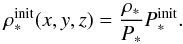16)In a similar vein, we get for the planet ${\mathit{P}}_{\mathrm{◦}}^{\mathrm{init}}\mathrm{\left(}\mathit{x,y,z}\mathrm{\right)}\mathrm{=}{\mathit{P}}_{\mathrm{◦}}\exp \left[{\mathit{\lambda }}_{\mathrm{◦}}\left(\frac{{\mathit{R}}_{\mathrm{◦}}}{{\mathit{R}}^{\mathrm{\prime }}}\mathrm{-}\mathrm{1}\right)\mathrm{-}\frac{\mathrm{1}}{\mathrm{2}}{\left(\frac{{\mathit{v}}_{\mathrm{w}\hspace{0.17em}\mathrm{◦}}^{\mathrm{init}}\mathrm{\left(}{\mathit{R}}^{\mathrm{\prime }}\mathrm{\right)}}{{\mathit{c}}_{\mathrm{s}\hspace{0.17em}\mathrm{◦}}}\right)}^{\mathrm{2}}\right]$(17)and ${\mathit{\rho }}_{\mathrm{◦}}^{\mathrm{init}}\mathrm{\left(}\mathit{x,y,z}\mathrm{\right)}\mathrm{=}\frac{{\mathit{\rho }}_{\mathrm{◦}}}{{\mathit{P}}_{\mathrm{◦}}}{\mathit{P}}_{\mathrm{◦}}^{\mathrm{init}}\mathit{.}$(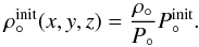18)We set up the stellar wind everywhere in the computational box, apart from a sphere of radius 10R_°, centered on the planet. Within this volume we initialize the planetary wind. Both outflows are initially supersonic and super-Alfvénic (with the Alfvén speed given by v_A = (B²/ 4πρ)^{1 / 2}) at the interface that separates them².

It is worth noting that the Parker wind (Eq. (7)) is nondimensional (with the radial distance expressed in units of the radius of the object and the velocity in units of the sound speed at the base) and that its solution depends only on the parameter λ, which can be written in the form 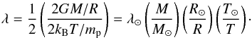$\mathit{\lambda }\mathrm{=}\frac{\mathrm{1}}{\mathrm{2}}\left(\frac{\mathrm{2}\mathit{GM}\mathit{/}\mathit{R}}{\mathrm{2}{\mathit{k}}_{\mathrm{B}}\mathit{T}\mathit{/}{\mathit{m}}_{\mathrm{p}}}\right)\mathrm{=}{\mathit{\lambda }}_{\mathrm{\odot }}\left(\frac{\mathit{M}}{{\mathit{M}}_{\mathrm{\odot }}}\right)\left(\frac{{\mathit{R}}_{\mathrm{\odot }}}{\mathit{R}}\right)\left(\frac{{\mathit{T}}_{\mathrm{\odot }}}{\mathit{T}}\right)\mathrm{·}$(19)Interestingly, for a solar analog (R_∗ = 1 R_⊙, M_∗ = 1 M_⊙, T_∗ = 10⁶ K) and a hot Jupiter (R_° = 1 R_J ≃ 10^-1R_⊙, M_° = 1 M_J ≃ 10^-3M_⊙, T_° = 10⁴ K) we obtain λ_∗ ≈ λ_°. As a result, the two outflows reach their corresponding sonic speeds at the same scaled distance. For the adopted fiducial parameters, λ = 11.5, which implies that the stellar and planetary outflows become supersonic at a radius that is slightly smaller than 6R_∗ and 6R_°, respectively.

In a real system, the stellar flux that heats the planetary surface varies with longitude (in particular, there is no direct irradiation of the planet’s night side) as well as latitude (in particular, the planetary poles also receive no direct heating). This implies that even an unmagnetized outflow would be anisotropic, although the quantitative effect of the uneven irradiation on the evaporative mass outflow rate need not be large (e.g., Murray-Clay et al. 2009). In this work we simplify the treatment by assuming that the base temperature and density are uniform over the entire planetary surface.

The initial magnetic field configuration in the computational domain is taken to be a sum of two magnetic dipoles, ${{B}}_{\mathrm{\ast }}^{\mathrm{init}}\mathrm{+}{{B}}_{\mathrm{◦}}^{\mathrm{init}}$, which are given by ${{B}}_{\mathrm{\ast }}^{\mathrm{init}}\mathrm{\left(}\mathit{x,y,z}\mathrm{\right)}\mathrm{=}\frac{{\mathit{B}}_{\mathrm{\ast }}{\mathit{R}}_{\mathrm{\ast }}^{\mathrm{3}}}{{\mathit{R}}^{\mathrm{5}}}\mathrm{[}\mathrm{3}\mathit{xz}\hspace{0.17em}\mathit{x̂}\mathrm{+}\mathrm{3}\mathit{yz}\hspace{0.17em}\mathit{ŷ}\mathrm{+}\mathrm{(}\mathrm{3}{\mathit{z}}^{\mathrm{2}}\mathrm{-}{\mathit{R}}^{\mathrm{2}}\mathrm{)}\hspace{0.17em}\mathit{ẑ}\mathrm{]}$(20)and ${{B}}_{\mathrm{◦}}^{\mathrm{init}}\mathrm{\left(}\mathit{x,y,z}\mathrm{\right)}\mathrm{=}\frac{{\mathit{B}}_{\mathrm{◦}}{\mathit{R}}_{\mathrm{◦}}^{\mathrm{3}}}{{\mathit{R}}^{\mathrm{\prime }\mathrm{5}}}\mathrm{[}\mathrm{3}{\mathit{x}}^{\mathrm{\prime }}{\mathit{z}}^{\mathrm{\prime }}\hspace{0.17em}\mathit{x̂}\mathrm{+}\mathrm{3}{\mathit{y}}^{\mathrm{\prime }}{\mathit{z}}^{\mathrm{\prime }}\hspace{0.17em}\mathit{ŷ}\mathrm{+}\mathrm{(}\mathrm{3}{\mathit{z}}^{\mathrm{\prime }\mathrm{2}}\mathrm{-}{\mathit{R}}^{\mathrm{\prime }\mathrm{2}}\mathrm{)}\hspace{0.17em}\mathit{ẑ}\mathrm{]}$(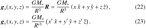21)for the star and planet, respectively. Both dipoles are oriented along the z axis and are aligned with each other. We also include the components of the total gravitational field g outside the two bodies in the form

$\begin{array}{ccc}& & {{g}}_{\mathrm{\ast }}\mathrm{\left(}\mathit{x,y,z}\mathrm{\right)}\mathrm{=}\frac{\mathit{G}{\mathit{M}}_{\mathrm{\ast }}}{{\mathit{R}}^{\mathrm{3}}}{R}\mathrm{=}\frac{\mathit{G}{\mathit{M}}_{\mathrm{\ast }}}{{\mathit{R}}^{\mathrm{3}}}\left(\mathit{x}\hspace{0.17em}\mathit{x̂}\mathrm{+}\mathit{y}\hspace{0.17em}\mathit{ŷ}\mathrm{+}\mathit{z}\hspace{0.17em}\mathit{ẑ}\right)\mathit{,}\\ & & {{g}}_{\mathrm{◦}}\mathrm{\left(}\mathit{x,y,z}\mathrm{\right)}\mathrm{=}\frac{\mathit{G}{\mathit{M}}_{\mathrm{◦}}}{{\mathit{R}}^{\mathrm{\prime }\mathrm{3}}}\left({\mathit{x}}^{\mathrm{\prime }}\hspace{0.17em}\mathit{x̂}\mathrm{+}{\mathit{y}}^{\mathrm{\prime }}\hspace{0.17em}\mathit{ŷ}\mathrm{+}{\mathit{z}}^{\mathrm{\prime }}\hspace{0.17em}\mathit{ẑ}\right)\mathit{.}\end{array}$

2.4. Wind boundary conditions

In order to continuously accelerate the outflows and guarantee a constant supply of mass, we keep fixed the density, pressure, and velocity at their bases. Specifically, during the temporal evolution, we impose the initial values of these quantities at the regions defined by R_∗<R< 1.5 R_∗ and R_°<R′< 1.5 R_° for the stellar and planetary winds, respectively. However, the magnetic field is free to evolve within these shells, readjusting self-consistently from its initial dipolar topology. This is a simplified treatment as compared with the formulation of Matt & Pudritz (2008), who modeled 2.5D axisymmetric stellar winds using a thinner, four-layer shell above the surface of the star³. Within that region, they progressively relaxed the time-dependency constraint on the physical quantities. Here we employ a less detailed setup on account of the lower resolution imposed by our 3D modeling. Nevertheless, the steady-state winds that we obtain compare well with the more refined 2.5D simulations (see Sect. 2.8).

The above implementation of stellar winds differs from the approach adopted by Cohen et al. (2011a,b, 2014) and Vidotto et al. (2014, and references therein), which includes nonaxisymmetric and/or temporal variabilities. We neglect such effects in this work in order to investigate the star–planet interaction in a general manner that does not depend on temporary local fluctuations.

Our wind boundary conditions do not incorporate the effect of tidal forces on the planetary outflow. As discussed by Trammell et al. (2011), these forces could suppress the wind from the polar regions of a tidally locked planet with a dipolar field geometry. In particular, these authors showed that the wind would not undergo a sonic transition in this case if ${\mathit{ϵ}}_{\mathrm{◦}}\mathit{>}\mathrm{4}\mathit{/}{\mathit{\lambda }}_{\mathrm{◦}}^{\mathrm{2}}$ (where the parameters ϵ and λ are defined in Sect. 2.2). Our neglect of this suppression in the adopted boundary conditions is not a serious omission because our simulations incorporate the effect of these forces for R′ ≥ 1.5 R_° and because the sonic surface typically lies at a distance of a few R_° from the planet’s center⁴. Furthermore, for the star–planet configurations considered in this paper, which are characterized by parallel orbital and spin axes, the bulk of the interaction between the stellar and the planetary plasmas occurs in the equatorial plane, with the details of the planetary outflow from the polar regions having little effect on the results.

2.5. Stellar and planetary interiors

The interiors of both the star and the planet are treated as an internal boundary. In particular, the values of all physical quantities are kept fixed by having them overwritten at each time step. To avoid spurious effects at the surfaces of the objects, or extreme dynamics that could affect the global time step of the simulation, we prescribe an approximate equilibrium within their volumes.

Since the physical conditions in the interior of the star or the planet are not important for the simulation, the simplest approach is to consider them as uniform-density spheres. The interior gravitational accelerations are then given by ${{g}}_{\mathrm{\ast }}\mathrm{\left(}\mathit{x,y,z}\mathrm{\right)}\mathrm{=}\frac{\mathrm{4}}{\mathrm{3}}\mathit{\pi G}{\mathit{\rho }}_{\mathrm{\ast }}{R}\mathrm{=}\frac{\mathrm{4}}{\mathrm{3}}\mathit{\pi G}{\mathit{\rho }}_{\mathrm{\ast }}\mathrm{(}\mathit{x}\hspace{0.17em}\mathit{x̂}\mathrm{+}\mathit{y}\hspace{0.17em}\mathit{ŷ}\mathrm{+}\mathit{z}\hspace{0.17em}\mathit{ẑ}\mathrm{)}$(24)and ${{g}}_{\mathrm{◦}}\mathrm{\left(}\mathit{x,y,z}\mathrm{\right)}\mathrm{=}\frac{\mathrm{4}}{\mathrm{3}}\mathit{\pi G}{\mathit{\rho }}_{\mathrm{◦}}\mathrm{(}{\mathit{x}}^{\mathrm{\prime }}\mathit{x̂}\mathrm{+}{\mathit{y}}^{\mathrm{\prime }}\mathit{ŷ}\mathrm{+}{\mathit{z}}^{\mathrm{\prime }}\mathit{ẑ}\mathrm{)}\mathit{,}$(25)from which the pressures can be inferred using the hydrostatic equilibrium condition:

$\begin{array}{ccc}{\mathit{P}}_{\mathrm{\ast }}^{\mathrm{init}}\mathrm{\left(}\mathit{x,y,z}\mathrm{\right)}\mathrm{=}{\mathit{P}}_{\mathrm{\ast }}\mathrm{+}\frac{\mathrm{2}}{\mathrm{3}}\mathit{\pi G}{\mathit{\rho }}_{\mathrm{\ast }}^{\mathrm{2}}\mathrm{(}{\mathit{R}}_{\mathrm{\ast }}^{\mathrm{2}}\mathrm{-}{\mathit{R}}^{\mathrm{2}}\mathrm{)}\mathit{,}& & \\ {\mathit{P}}_{\mathrm{◦}}^{\mathrm{init}}\mathrm{\left(}\mathit{x,y,z}\mathrm{\right)}\mathrm{=}{\mathit{P}}_{\mathrm{◦}}\mathrm{+}\frac{\mathrm{2}}{\mathrm{3}}\mathit{\pi G}{\mathit{\rho }}_{\mathrm{◦}}^{\mathrm{2}}\mathrm{(}{\mathit{R}}_{\mathrm{◦}}^{\mathrm{2}}\mathrm{-}{\mathit{R}}^{\mathrm{\prime }\mathrm{2}}\mathrm{)}\mathit{.}& & \end{array}$We keep the dipolar expression for the magnetic field, but we smooth it out at the center where it becomes singular. Specifically, we assume that the central regions of the star and the planet, R<R_∗/ 2 and R′<R_°/ 2, are uniformly magnetized spheres, with magnetic fields ${{B}}_{\mathrm{\ast }}^{\mathrm{init}}\mathrm{=}\mathrm{16}{\mathit{B}}_{\mathrm{\ast }}\hspace{0.17em}\mathit{ẑ}$ and ${{B}}_{\mathrm{◦}}^{\mathrm{init}}\mathrm{=}\mathrm{16}{\mathit{B}}_{\mathrm{◦}}\hspace{0.17em}\mathit{ẑ}$ that connect smoothly with the dipolar configurations at larger radii. Finally, we approximate the star and the planet as rotating rigid bodies and specify their angular velocities by Ω_∗ = Ω_∗ẑ and Ω_° = Ω_°ẑ, respectively.

2.6. The models

Table 2 lists the models that we study numerically. We aim to explore the observationally relevant regions of parameter space and attempt to deduce, based on the behaviors exhibited by the simulated systems, a general – and largely model-independent – classification scheme for magnetized star–planet interactions. We usually adopt two representative values for each of the physical variables that need to be specified in the model. Thus, we consider two combinations of planetary parameters, the first having Jupiter’s mass and radius and the other corresponding to a less massive (0.5 M_J) and larger-radius (1.5 R_J) planet. These choices are intended to sample the typical range of values for the escape speed v_{esc °} ∝ (M_°/R_°)^{1 / 2} from a hot Jupiter, which is relevant to the mass evaporation process.

We similarly consider two magnitudes for the UV flux, one low (F_UV = 5 × 10² erg cm^-2 s^-1) and one high (F_UV = 5 × 10⁵ erg cm^-2 s^-1), adopting numerical values similar to those given for these two limits in Murray-Clay et al. (2009). These two values correspond to different evaporation regimes. In the high-flux case, the excess photoionization energy is largely lost by radiative cooling (radiation/recombination-limited evaporation), whereas in the low-flux case it is mostly absorbed and drives the outflow (energy-limited evaporation). The outflow from a strongly irradiated planet is denser, hotter, and faster than that from a weakly irradiated one (e.g., Murray-Clay et al. 2009). Since in this paper we do not explicitly model the radiative processes in the planetary atmosphere, we specify the wind properties through the values of the base temperature and density, which are adjusted to match the results of more detailed calculations (see Sect. 2.8).

We also vary the distance of the hot Jupiter from the host star. Smaller orbital radii imply a stronger tidal force as well as a locally weaker, and possibly not fully developed, stellar wind⁵. The value of the orbital radius also determines whether the planet lies within the critical surface of the stellar wind or whether it is impacted by a super-critical flow.

The two values that we adopt for the magnetic field amplitude at the planet’s surface differ by an order of magnitude and are intended to represent a strong and a weak field. Stronger fields correspond to higher magnetic pressure and tension and exhibit greater effective rigidity. In this case the field resists being opened up by the stellar outflow over a larger region near the equator, and as a result the planetary magnetosphere presents a larger obstacle in its interaction with the stellar wind.

Although we vary the stellar UV flux, our simulations employ only a single set of stellar wind parameters. Our coverage of the relevant parameter phase space is, however, sufficiently broad to yield general results, which in principle apply also to systems with either a weaker or a stronger stellar wind.

2.7. Numerical setup

The simulations are performed with PLUTO (version 4.0.1), a code for computational astrophysics (Mignone et al. 2007, 2012)⁶. The computational domain consists of a cube, with x,y,z ∈ [−15, 15] R_∗, which is resolved by a static, multiply refined grid of 224 × 192 × 192. We have also carried out one simulation (model FvRb) in higher resolution, 424 × 320 × 320, in order to validate our results. The region around the star, x,y,z ∈ [−5, 5] R_∗, is resolved with Δx, Δy, Δz ≃ 0.16 R_∗ (64³ cells) in most cases, and with Δx, Δy, Δz ≃ 0.08 R_∗ (128³ cells) in the high-resolution simulation. However, for the hot Jupiter and its surroundings, x′,y′,z′ ∈ [−5, 5] R_°, we use a resolution that is higher by one order of magnitude, i.e., Δx, Δy, Δz ≃ 0.016 R_∗ (64³ cells) and Δx, Δy, Δz ≃ 0.008 R_∗ (128³ cells) for the standard and highly resolved cases, respectively. In the region between the star and the planet we apply the resolution Δx,Δy,Δz ≃ 0.16 R_∗.

The total time of the simulation is typically ~4 days, only a fraction of which is required for the system to attain a quasi-steady state. For comparison, a stellar wind propagating at 300 km s^-1 travels ~10 times the distance from the star to the outer boundary over this time interval. We adopt highly accurate numerical schemes to compensate for the resolution limits imposed by the 3D character of the simulations. In particular, we use the HLLD Riemann solver and apply third-order accuracy in space (piecewise parabolic interpolation) and time (3rd order Runge-Kutta). The condition ∇·B = 0 is implemented using the divergence-cleaning method, an approach based on the generalized Lagrange multiplier (GLM) formulation (see Mignone et al. 2012 and references therein).

2.8. Verification and calibration of 3D wind models

The acceleration and final steady-state properties of a simulated wind depend on the included physics as well as on the resolution of the grid. 3D simulations are computationally expensive and therefore cannot incorporate the same level of detail that is possible in 1D and 2D models. In this work we have implemented a simplified procedure for treating the stellar and planetary outflows, and we now check on the validity of the adopted approximations. We first compare our 3D stellar-wind model with a more detailed (and higher-resolution) 2.5D model and verify its consistency. We then demonstrate our method of ensuring the consistency of 3D planetary wind models with 1D hydrodynamic calculations that incorporate the relevant physics of evaporative outflows.

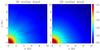Fig. 1 Logarithmic density contours, field lines (solid lines), and poloidal Alfvén surface (dashed line) in the final steady state of the 3D stellar wind model employed in this paper (left panel) and of a 2.5D high-resolution simulation (right panel).

Figure 1 compares the 3D stellar wind model adopted in this work (left panel) with a 2.5D simulation that employs the same parameters (right panel) but has a 10 times higher resolution along each direction (modeled as in Matt & Pudritz 2008). The density, velocity, and magnetic field have very similar profiles in spite of the fact that every cell on the left would be resolved by a thousand cells on the right if it were a 3D setup. Any discrepancies can be neglected since the outflow serves its purpose of providing a generic stellar wind.

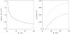Fig. 2 Logarithmic density (left) and radial velocity (right) in the final steady state of the 3D stellar wind model as a function of the distance R from the center of the star along the equatorial (x) and axial (z) directions (solid and dashed lines, respectively).

Figure 2 shows the profiles of the density (left panel) and radial velocity (right panel) for the steady state reached by our stellar wind model. The radial velocity is zero along the equator up to ~4R_∗, corresponding to the extent of the stellar dead zone (see Fig. 1). More generally, the finding that the wind speed remains lower along x than along z for any given value of R can be attributed to the fact that a smaller fraction of the field lines open up near the equator than near the poles. This behavior is also exhibited by more detailed models of winds from solar-type stars (e.g., Cohen & Drake 2014). In the case of faster rotators, in which magnetocentrifugal effects play a more prominent role in the acceleration of the wind, the outflow speed along the equator can become higher than along the spin axis (e.g., Matt & Pudritz 2008). This regime is pertinent to our models of tidally locked planets.

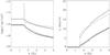Fig. 3 Logarithmic density (left) and radial velocity (right) as a function of distance from the planet’s center for the isotropic outflow model used to initialize the 3D wind simulation for a “light” hot Jupiter (M° = 0.5 MJ, R° = 1.5 RJ). The symbols “+” and “×” denote, respectively, the high- and low-flux cases (modeled with T° = 104 K and T° = 6 × 103 K, respectively). The solid and dashed lines are from the corresponding 1D simulations that take into account the relevant heating and cooling processes (see text for details).

To ensure that the planetary winds are properly initialized, we specify the boundary conditions so that the resulting profiles match the results of a more elaborate (and highly resolved) 1D model that incorporates relevant additional physics. Specifically, we simulate the outflow along the line joining the centers of the planet and the star, incorporating explicit energy and ionization balance equations following the formulation of Murray-Clay et al. (2009). The energy equation includes advective and PdV-work terms as well as source terms in the form of photoionization heating (assuming a single ionizing photon energy of 20 eV and perfect efficiency) and Lyα cooling (under the assumption of collisional excitation by free electrons). This equation is integrated using a modified version of the Simplified Non-Equilibrium Cooling (SNEq) module of PLUTO (Teşileanu et al. 2008). The hydrogen ionization balance equation accounts for photoionization, Case B radiative recombination, and ion advection. Using the results of these calculations, we fine-tuned the boundary conditions of the simplified 3D models until the latter were found to effectively capture the general features of the 1D models for our representative planets in both the high- and low-flux limits. The steady-state planetary wind profiles obtained in this way are shown in Figs. 3 and 4 together with the corresponding 1D results.

As can be seen from Figs. 3 and 4, the 1D outflow models predict a very steep density drop near the surface of the planet. This implies that, if one were to choose the value of the surface density ρ_° for the 3D simulation simply on the basis of the location of the nominal base of the flow (where τ ~ 1), this would likely not lead to a good match with the 1D density profile. On the other hand, if one were to choose even a slightly different reference radius for fixing the surface density, this might result in a significant under- or over-estimate of the mass outflow rate. These considerations strongly suggest that the correct procedure for modeling the underlying planetary outflow is to choose the boundary values of density and temperature on the surface of the planet so that they lead to a good match with the reference profiles. The small discrepancy seen in the velocity profile of the low-flux case in Fig. 4 can be ignored because, as we show below, the interaction with the stellar plasma chokes the outflow from a Jupiter-like planet for this value of the flux.

Fig. 4 Same as Fig. 3, but for a Jupiter-like planet (M° = MJ, R° = RJ).

3. Numerical results

3.1. Unmagnetized star–planet interactions

Before turning to the MHD simulations, we make a few qualitative remarks on the expected behavior in the absence of magnetic fields. Assuming that there is no planetary outflow, the stellar wind will impact the planet directly. For a supersonic stellar flow, the height above the planet’s surface where the plasma will get shocked is determined by the location where the atmospheric thermal pressure, P_{th °}, is equal to the local value of the wind ram pressure, ${\mathit{\rho }}_{\mathrm{w}\hspace{0.17em}\mathrm{\ast }}{\mathit{v}}_{\mathrm{w}\hspace{0.17em}\mathrm{\ast }}^{\mathrm{2}}$. For a subsonic flow, there will be no shock, but rather a smooth transition of the physical quantities between the two bodies: the density and pressure will have high values at the surface of each object and will be lower in between. The converse will hold for the velocity: zero values at the surfaces, and a smooth acceleration – and subsequent deceleration – on moving from the host to the hot Jupiter.

If a planetary outflow is present, its strength will determine whether it will be suppressed by the stellar wind (weak outflow) or else become supersonic and then collide with the stellar plasma well away from the planet’s surface (strong outflow). When both flows are supersonic, they interact at the location where the ram pressure of the planetary wind, ${\mathit{\rho }}_{\mathrm{w}\hspace{0.17em}\mathrm{\ast }}{\mathit{v}}_{\mathrm{w}\hspace{0.17em}\mathrm{\ast }}^{\mathrm{2}}$, is equal to that of the stellar gas (as measured in the corotating frame).

3.2. General behavior

We start our presentation of the MHD simulations by describing the general structure of the interacting outflows; in the ensuing subsections we present the results for each of the simulated models in greater detail.

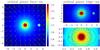Fig. 5 Initial conditions in the lab frame for model FVRB. The axes are in units of 0.01 AU. Logarithmic density contours (in units of g cm-3) are shown in the x-y plane (z = 0; left panel) and in the x-z plane (y = 0; right panels). The top right panel is focused on the star and the bottom right on the planet. Solid lines represent the magnetic field, arrows show the velocity field (with the longest one corresponding to ~290 km s-1), dashed lines the poloidal Alfvén surface (${\mathit{v}}_{\mathit{x}}^{\mathrm{2}}\mathrm{+}{\mathit{v}}_{\mathit{z}}^{\mathrm{2}}\mathrm{=}\mathrm{(}{\mathit{B}}_{\mathit{x}}^{\mathrm{2}}\mathrm{+}{\mathit{B}}_{\mathit{z}}^{\mathrm{2}}\mathrm{)}\mathit{/}\mathrm{4}\mathit{\pi \rho }$), and dotted lines the poloidal sonic surface (${\mathit{v}}_{\mathit{x}}^{\mathrm{2}}\mathrm{+}{\mathit{v}}_{\mathit{z}}^{\mathrm{2}}\mathrm{=}\mathit{\gamma P}\mathit{/}\mathit{\rho }$). The cross in the bottom right panel denotes the location of the L1 point.

We use model FVRB for this illustration, and show its initial configuration in Fig. 5; the initial structure of the other models is similar except for the planetary wind profiles, which depend on the choice of surface parameters (see Figs. 3 and 4). The star is located at the center of the left panel and of the top right panel, which respectively provide face-on and edge-on views of the orbital plane. The stellar wind is depicted with arrows, and its initially dipolar magnetic field with solid lines. Next to the star, at x ~ 4.5 (in units of 0.01 AU), is the spherical volume within which the hot Jupiter and its outflow are located (left and top right panels). A close-up of the region near the planet is shown in the bottom right panel. We note that both the stellar and the planetary winds are super-Alfvénic and supersonic at the initial interface between them (a sphere of radius 10R_°, centered on the planet).

At the beginning of the simulation, the plasma escaping from the surface of each object forces the magnetosphere to open. In general, depending on the strength of the magnetic field and the physical conditions at the base of the wind, this might happen over the entire surface (for a weaker field and/or a stronger outflow) or just at the polar regions (for a stronger field and/or a weaker outflow). For the adopted value of the stellar surface magnetic field (B_∗ = 2 G), the star forms a dead zone for π/ 4 ≲ θ ≲ 3π/ 4. In this region, the hot plasma cannot overcome the opposing forces of stellar gravity and magnetic tension, both of which are almost perpendicular to the flow. The behavior of the planetary magnetosphere will be discussed on a case by case basis: its structure depends both on B_° and the planetary wind properties and on its environment.

3.3. Models exhibiting a planetary tail

Figure 6 shows the final steady state of model fvRb. This case corresponds to a low UV flux, and the planetary outflow is weak and cannot overcome the ram pressure of the stellar wind (projected along the orbit). The stellar wind is stopped by the magnetic pressure of the planet’s closed field lines (which exceeds the thermal pressure above the planet’s surface), terminating in a bow shock that stands off a few planetary radii from the planet’s surface. The magnetosphere is dragged backward by the stellar wind, forming a cometary-type tail. This process is akin to the formation of the geomagnetic tail in the interaction of the solar wind with Earth’s magnetosphere (e.g., Ness 1965). The tail does not follow the trajectory of the planet since it is continuously pushed away radially by the stellar wind, resulting in a tilted structure.

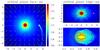Fig. 6 Logarthimic density (color contours in units of g cm-3), velocity (arrows), magnetic field (solid lines), critical surfaces (dotted line: sonic, dashed line: Alfvén), and the L1 point (cross) for the final steady state of model fvRb. Distances are measured in units of 0.01 AU. The panels are arranged as in Fig. 5, with the left and top right panels centered on the star, and the bottom right one on the planet.

Fig. 7 Same as the left panel of Fig. 6, but for models fvRB (left) and FVRb (right).

Figure 7 illustrates how the structure of the tail is modified when the model parameters are changed. The left panel shows the results for model fvRB, which has the same parameters as model fvRb (Fig. 6) except that the planetary magnetic field is a factor of 10 stronger, corresponding to an increase by a factor of 100 in the magnetic pressure at a given distance from the planet. As expected, this results in the bow shock being located farther away from the planetary surface, which, in turn, gives rise to a wider tail. The right panel presents the final state for model FVRb, which corresponds to a higher UV flux (which promotes an outflow) but also a larger escape speed (which hinders a wind). Overall, its behavior is very similar to that of model fvRb, although the tail in this case is noticeably denser. This can be understood from the fact that, in the high-flux limit, the base density scales roughly as ${\mathit{F}}_{\mathrm{UV}}^{\mathrm{1}\mathit{/}\mathrm{2}}{\mathit{v}}_{\mathrm{esc}\hspace{0.17em}\mathrm{◦}}$ (Murray-Clay et al. 2009).

The snapshot shown in the right panel of Fig. 7 highlights a few interesting dynamical features of cometary-type tails. The plasma that trails the planet has a velocity comparable to the orbital speed, whereas the component of the stellar wind along the orbit is negligible at that location. This results in the development of strong shear, which may trigger a Kelvin-Helmholtz instability. Furthermore, the stellar plasma that pushes the tail outward is of lower density than the trailing stream, which can induce a Rayleigh-Taylor instability. In this particular simulation, their effect on the tail structure remains comparatively mild, likely on account of the relatively high density of the trailing stream. We have, however, found that the induced distortions can be more persistent in other cases.

Fig. 8 Same as Fig. 6, but for model fVRb.

When the UV flux remains low but the escape speed is high, the planetary outflow weakens and the density in the tail becomes measurably lower than in the models considered so far. This result follows directly from the inferred scaling of the mass evaporation rate in the low-flux limit, $\mathit{Ṁ}{}_{\mathrm{ev}}\mathrm{\propto }{\mathit{F}}_{\mathrm{UV}}\mathit{/}{\mathit{v}}_{\mathrm{esc}}^{\mathrm{2}}$ (Eq. (9) in Murray-Clay et al. 2009). In this case the tail becomes thin and barely noticeable, as demonstrated in Fig. 8 for model fVRb. The outflow is even weaker when the magnetic field amplitude is increased (model fVRB, not plotted).

3.4. Models exhibiting both a tail and an accretion stream

Fig. 9 Same as Fig. 6, but for model FvRb.

Figures 9 and 10 show the final quasi-steady state of model FvRb. This model differs from the reference case of Sect. 3.3 (model fvRb, shown in Fig. 6) in having a high (rather than low) incident UV flux. This results in the formation of a strong outflow, which opens up the magnetosphere and becomes supersonic (bottom right panel)⁷.

The planetary outflow propagates unperturbed over a few planetary radii, giving rise to the eye-shaped region around the planet at 4.0 ≲ x ≲ 5.5 (left and top right panels of Fig. 9). Beyond that region, the planetary outflow collides with the stellar wind and forms a shock. This happens on both the day and night sides of the hot Jupiter on account of the high orbital speed (which shifts the apex of the bow shock away from the substellar point) and the axisymmetry assumption for the planetary wind.

A noteworthy feature of the interaction in this case is the accretion of part of the shocked planetary outflow onto the host star. The infalling material spirals for a quarter of an orbit and then impacts the stellar surface. The fact that this gas falls in, rather than forming a torus-like structure, can be attributed to the action of the shock and of the stellar wind, which slow down and disrupt the flow, and to the increase in the gravitational pull of the star as the gas spirals in. The rest of the outflowing planetary gas is, however, pushed back and forms a tail, as in the cases considered in the preceding subsection. Both the inspiraling and the trailing streams are affected by the velocity shear with the low-density stellar gas and by the outward acceleration that this component induces, which trigger Kelvin-Helmholtz and Rayleigh-Taylor instabilities. These effects lead to the destruction of the tail in this case, with its fragments being pushed outward by the ram pressure of the stellar wind (left panel of Fig. 9). A very similar outcome is produced for model FvRB (not plotted), in which, however, the stronger planetary magnetic field results in the Alfvén surface lying farther away from the planet than the sonic one.

Accretion streams onto the stellar surface can form also in cases where the planetary outflow remains weak and the stellar wind is stopped by the planetary magnetic field. This is illustrated in Fig. 11, which shows the final configuration of model FVRB. This case is similar to model FVRb, shown in the right panel of Fig. 7, in that a combination of high UV flux and large escape speed generate a dense discharge from the planetary surface but only a weak outflow. In this case, however, the stronger magnetic field causes the interface between the planetary magnetosphere and the shocked stellar wind to lie at a larger distance from the planet’s surface; in particular, it now lies beyond the L₁ point. At that location, the gravitational pull from the star and the thermal pressure of the dead zone combine to deform the planetary magnetic field lines in such a way that accretion streams are formed. In general, accretion streams do not flow smoothly: as is seen in the left panels of Figs. 9 and 11, their interaction with the stellar wind and the magnetic field of the star causes their trajectories to split several times before they reach the stellar surface.

A similar situation characterizes our high-flux “near” models, as illustrated in Fig. 12 with model FvrB. In this case, the planetary outflow is massive enough and the L₁ point is located close enough to the planet’s surface that both a planetary tail and an accretion stream are formed, resembling the behavior of model FVRB. However, the different position of the planet relative to the star modifies the evolution in this case. First, the fragmented tail is not pushed away by the stellar outflow, which is still weak at this location. Instead, the stellar outflow mixes with these fragments and slows them down, leading to their accretion by the star. Second, the denser ambient stellar gas in this model also enhances the mixing with the accretion stream, slowing the latter down and causing it to hit the stellar surface close to the orbital location of the planet. Finally, as the orbital motion of the planet is now faster than the stellar field-line rotation, the stream does not attain a steady-state configuration. Instead, the magnetic field topology undergoes a continuous readjustment, with new magnetic accretion channels forming periodically. Model FVrB (not plotted) exhibits a similar morphology to that of model FvrB, with accretion flows onto the star originating from both the upstream and downstream regions of the planet, although the larger escape speed results in less mass leaving the planet in this case. We however find that there is no transfer of mass to the star when the UV flux is low, irrespective of whether the escape speed is large or small (models fVrB and fvrB, respectively; these are also not plotted).

4. Classification of star–planet interactions

Our simulations of the dynamical interaction between a magnetized, wind-driving host star and a magnetized hot Jupiter that loses mass to photoevaporation were described in Sect. 3 in terms of the resulting morphological structures. We now attempt to distill from this phenomenology a general classification scheme that is based on the underlying dynamical processes operating in such systems. We quantify the relative influence of these processes with the help of characteristic length scales, and use the latter to identify four basic types of interaction. We then apply this scheme to the categorization of the models listed in Table 2.

4.1. Characteristic length scales

The formation of a quasi-stationary morphological structure in the interaction between a star and a close-in planet entails the establishment of pressure equilibrium between the stellar and planetary plasmas at the interface separating these two media⁸. The relevant frame of reference for considering this equilibrium is that of the planet, and we label the pressure on the stellar side of the boundary in this frame by P_amb. The characteristic distance of this surface from the center of the planet, measured along (or close to) the line to the stellar center, is determined by whether it is the magnetic pressure, outflow ram pressure, or thermal pressure that dominates on the planet’s side of the boundary.

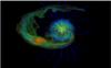Fig. 10 3D representation of the density structure and of the magnetic field lines (blue: stellar; red: planetary) for model FvRb. The logarithmic density scale is chosen for visualization purposes and does not correspond to that of Fig. 9.

Fig. 11 Same as Fig. 6, but for model FVRB.

Fig. 12 Same as Fig. 6, but for model FvrB.

If the pressure of a closed planetary magnetosphere dominates, we can estimate the relevant scale (R_m) by assuming a dipolar field, B_°(R′) = B_°(R_°/R′)³, and equating its pressure ${\mathit{P}}_{\mathrm{mag}\hspace{0.17em}\mathrm{◦}}\mathrm{=}{\mathit{B}}_{\mathrm{◦}}^{\mathrm{2}}\mathrm{\left(}{\mathit{R}}^{\mathrm{\prime }}\mathrm{\right)}\mathit{/}\mathrm{8}\mathit{\pi }$ to P_amb. This gives ${\mathit{R}}_{\mathrm{m}}\mathrm{=}{\left(\frac{{\mathit{B}}_{\mathrm{◦}}^{\mathrm{2}}{\mathit{R}}_{\mathrm{◦}}^{\mathrm{6}}}{\mathrm{8}\mathit{\pi }{\mathit{P}}_{\mathrm{amb}}}\right)}^{\mathrm{1}\mathit{/}\mathrm{6}}\mathrm{·}$(28)If, however, the planetary outflow is strong enough to become supercritical by the time it is stopped (in a shock) by colliding with the stellar gas, the relevant scale (R_w) is given, instead, by equating P_amb to the ram pressure ${\mathit{P}}_{\mathrm{ram}\hspace{0.17em}\mathrm{◦}}\mathrm{=}{\mathit{\rho }}_{\mathrm{w}\mathrm{◦}}{\mathit{v}}_{\mathrm{w}\mathrm{◦}}^{\mathrm{2}}$. Expressing the density in terms of the planetary mass loss rate Ṁ_° = 4πR^′2ρ_w°v_w°, we get 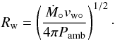${\mathit{R}}_{\mathrm{w}}\mathrm{=}{\left(\frac{\mathit{Ṁ}\mathrm{◦}{\mathit{v}}_{\mathrm{w}\mathrm{◦}}}{\mathrm{4}\mathit{\pi }{\mathit{P}}_{\mathrm{amb}}}\right)}^{\mathrm{1}\mathit{/}\mathrm{2}}\mathrm{·}$(29)Which of these pressure components (magnetic or ram) dominates the interaction with the stellar plasma is reflected in the relative magnitudes of the associated characteristic radii.

One could in principle also consider the contribution of the thermal pressure P = 2ρk_BT/m_p of the planetary atmosphere, but in practice its role is negligible because of its expected rapid decline with radius. In particular, under the isothermal approximation, P_°(R′) ∝ exp(λ_°R_°/R′) (see Eq. (17)), which represents a much faster drop than that of the magnetic pressure (P_mag ∝ (R_°/R′)⁶). In fact, the magnetic pressure likely already dominates the thermal pressure at the (subsonic) base of the planetary outflow, where, using Jupiter’s mass, radius, and magnetic field (B_° ≃ 4 G), and the base density (ρ_° ≃ 10^-14 g cm^-3) and temperature (T_° ≃ 10⁴ K) inferred from our high–UV-flux model (see Fig. 4), we estimate 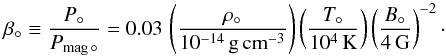${\mathit{\beta }}_{\mathrm{◦}}\mathrm{\equiv }\frac{{\mathit{P}}_{\mathrm{◦}}}{{\mathit{P}}_{\mathrm{mag}\hspace{0.17em}\mathrm{◦}}}\mathrm{=}\mathrm{0.03}\hspace{0.17em}\left(\frac{{\mathit{\rho }}_{\mathrm{◦}}}{{\mathrm{10}}^{-14}\hspace{0.17em}{\mathrm{g}\hspace{0.17em}\mathrm{cm}}^{-3}}\right)\left(\frac{{\mathit{T}}_{\mathrm{◦}}}{{\mathrm{10}}^{\mathrm{4}}\hspace{0.17em}\mathrm{K}}\right){\left(\frac{{\mathit{B}}_{\mathrm{◦}}}{\mathrm{4}\hspace{0.17em}\mathrm{G}}\right)}^{-2}\mathrm{·}$(30)We note, however, that when the stellar wind is stopped by a supercritical planetary wind, the plasma on the planet’s side of the contact discontinuity is dominated by its thermal pressure (having passed through a shock).

The ambient pressure can be approximated by the sum of four contributions, ${\mathit{P}}_{\mathrm{amb}}\mathrm{=}{\mathit{P}}_{\mathrm{w}\mathrm{\ast }}\mathrm{+}{\mathit{P}}_{\mathrm{mag}\hspace{0.17em}\mathrm{\ast }}\mathrm{+}{\mathit{P}}_{\mathrm{ram}\hspace{0.17em}\mathrm{\ast }}\mathrm{+}{\mathit{P}}_{\mathrm{ram}\hspace{0.17em}\mathrm{orb}}\mathit{,}$(31)which represent, respectively, the stellar plasma’s thermal, magnetic, and intrinsic ram pressure components, and the ram pressure associated with the relative motion between the planet and the ambient (stellar) gas. In this approximation, we take the direction of the stellar wind to be purely radial and the direction of the orbital motion to be purely azimuthal in the lab frame. If the stellar wind is supercritical, a bow shock will form at the interaction site. In the limit v_orb ≪ v_{w ∗}, the apex of this shock will lie along the line connecting the centers of the star and the planet, and the shock surface will be symmetric about this line. However, given that the orbital speeds of hot Jupiters are typically ≳100 km s^-1 and are thus highly supersonic with respect to the ambient gas, such a shock will form even when the stellar wind is still subcritical when it is stopped. In this case, however, the shock will be oriented at a finite angle to the aforementioned line (see Eq. (37) below), and its apex will be displaced away from this line (in the direction of the planet’s motion)⁹. For typical parameters, we expect that the last two terms in Eq. (31) constitute the dominant contributions to P_amb.

One other characteristic length scale for this problem is the tidal (or Hill) radius, 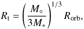${\mathit{R}}_{\mathrm{t}}\mathrm{=}{\left(\frac{{\mathit{M}}_{\mathrm{◦}}}{\mathrm{3}{\mathit{M}}_{\mathrm{\ast }}}\right)}^{\mathrm{1}\mathit{/}\mathrm{3}}{\mathit{R}}_{\mathrm{orb}}\mathit{,}$(32)which gives the distance of the L₁ Lagrange point from the planet’s center. This distance is relevant to the question of whether the morphology of the planetary gas that interacts with the stellar plasma will be shaped only by the relative motion between these two media (through the effect of the ram pressure terms in Eq. (31)) or whether the stellar gravitational field will also play a role. It can be expected that at least some of the planet’s plasma will be accreted onto the stellar surface if R_t< max(R_m,R_w), but that essentially all of the planet’s gas will remain confined to the vicinity of its orbital radius if this inequality is not satisfied.

Before concluding this subsection, we note that the components of P_amb can be expressed in terms of the stellar parameters just as was done above for the planet’s pressure components. In particular, assuming R_orb ≫ max(R_m,R_w) and using Ṁ_∗ = 4πR²ρ_{w ∗}v_{w ∗}, B_∗(R) = B_∗(R_∗/R)³, and the isothermal-gas approximation, we can express the terms appearing on the right-hand side of Eq. (31) in the form

$\begin{array}{ccc}& & {\mathit{P}}_{\mathrm{w}\mathrm{\ast }}\mathrm{=}\frac{\mathrm{2}{\mathit{\rho }}_{\mathrm{w}\mathrm{\ast }}{\mathit{k}}_{\mathrm{B}}{\mathit{T}}_{\mathrm{w}\mathrm{\ast }}}{{\mathit{m}}_{\mathrm{p}}}\mathrm{=}\frac{\mathit{Ṁ}\mathrm{\ast }{\mathit{k}}_{\mathrm{B}}{\mathit{T}}_{\mathrm{w}\mathrm{\ast }}}{\mathrm{2}\mathit{\pi }{\mathit{m}}_{\mathrm{p}}{\mathit{R}}_{\mathrm{orb}}^{\mathrm{2}}{\mathit{v}}_{\mathrm{w}\mathrm{\ast }}}\mathit{,}\\ & & {\mathit{P}}_{\mathrm{mag}\hspace{0.17em}\mathrm{\ast }}\mathrm{=}\frac{{\mathit{B}}_{\mathrm{\ast }}^{\mathrm{2}}}{\mathrm{8}\mathit{\pi }}{\left(\frac{{\mathit{R}}_{\mathrm{\ast }}}{{\mathit{R}}_{\mathrm{orb}}}\right)}^{\mathrm{6}}\mathit{,}\\ & & {\mathit{P}}_{\mathrm{ram}\hspace{0.17em}\mathrm{w}\mathrm{\ast }}\mathrm{=}{\mathit{\rho }}_{\mathrm{w}\mathrm{\ast }}{\mathit{v}}_{\mathrm{w}\mathrm{\ast }}^{\mathrm{2}}\mathrm{=}\frac{\mathit{Ṁ}\mathrm{\ast }{\mathit{v}}_{\mathrm{w}\mathrm{\ast }}}{\mathrm{4}\mathit{\pi }{\mathit{R}}_{\mathrm{orb}}^{\mathrm{2}}}\mathit{,}\\ & & {\mathit{P}}_{\mathrm{ram}\hspace{0.17em}\mathrm{orb}}\mathrm{=}{\mathit{\rho }}_{\mathrm{w}\mathrm{\ast }}{\mathit{v}}_{\mathrm{orb}}^{\mathrm{2}}\mathrm{=}\frac{\mathit{Ṁ}\mathrm{\ast }{\mathit{v}}_{\mathrm{orb}}^{\mathrm{2}}}{\mathrm{4}\mathit{\pi }{\mathit{R}}_{\mathrm{orb}}^{\mathrm{2}}{\mathit{v}}_{\mathrm{w}\mathrm{\ast }}}\mathrm{·}\end{array}$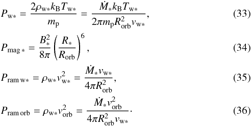Thus, the values of the three characteristic length scales (R_m, R_w, and R_t) can be estimated from a given set of planetary (R_°, M_°, Ṁ_°, v_w°, B_°), orbital (R_orb, v_orb), and stellar (R_∗, M_∗, Ṁ_∗, v_{w ∗}, T_{w ∗}, B_∗) parameters.

4.2. Types of interaction

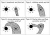Fig. 13 Schematic of the different possible star–planet interactions, showing face-on views in the orbital plane of the four distinct morphological structures (denoted by the Latin numerals I, II, III, and IV) as they appear in the planet’s frame. The large and small solid disks (on the left and right sides of each panel) represent the star and the hot Jupiter, respectively, the shaded areas highlight material that flowed out of the planet, the arrows indicate gas motions, and the closed loops sketch the planetary magnetosphere. The solid circular arcs in panels I and IV have a radius Rm, the distance where the magnetospheric pressure equals the total ambient pressure, whereas the dashed circular arcs in panels II and III mark the distance Rw where the ambient pressure equals the ram pressure of the planetary wind. The dotted line indicates the contour of the effective (gravity plus centrifugal) potential that passes through the Lagrange point L1 (at a distance Rt from the planet). The proposed classification scheme is based on the relative ordering of Rm, Rw, and Rt.

We base our classification of the flow structures that arise from the hydromagnetic interaction between a close-in giant planet and its host star on the relative magnitudes of the three characteristic length scales considered in Sect. 4.1: R_m, R_w, and R_t. The four basic types of interaction that we identify in this way are sketched in Fig. 13 and discussed below. We note, however, that any given system may not fall exclusively under a single category. This could be due to the planet having an eccentric orbit, to the stellar wind being nonaxisymmetric, or to the presence of multipolar components in the stellar magnetic field, each of which could lead to variations in the values of R_m and R_w on a timescale of ~days. A stellar magnetic cycle would be likely to induce variations on timescales of ~years in the properties of the stellar magnetic field, the stellar wind, and the stellar UV flux. Changes on even longer timescales could result from the effects of stellar evolution.

Type I: R _t > R _m > R _w

Type I interactions occur when the planetary outflow is weak (corresponding to either a low irradiating flux or a large escape speed), so that the stellar plasma is intercepted by the planetary magnetic field (i.e., R_m>R_w). As we noted in Sect. 4.1, the relative motion between the planet and the ambient gas is typically large enough to lead to the formation of a bow shock upstream of the planet. The shocked stellar flow sweeps back the planetary magnetic field and diverts the planetary outflow in the downstream direction, leading to the formation of a thin planetary tail. The stronger the planetary field, the larger its pressure – hence the farther away from the planetary surface does the shock appear (R_m is larger) and the wider the tail that is produced. The tail gas remains confined to the vicinity of the planet’s orbit because R_t>R_m.

The orientation of the tail is determined by the direction of the incident stellar wind as seen in the corotating frame at the apex of the bow shock. Approximating the wind velocity as being nearly radial in the lab frame and of magnitude v_w (see Fig. 5), the angle that the tail makes with respect to the tangent to the planet’s orbit (indicated on the top left drawing in Fig. 13) can be approximated by 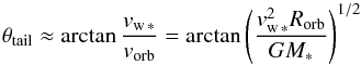${\mathit{\theta }}_{\mathrm{tail}}\mathrm{\approx }\arctan \frac{{\mathit{v}}_{\mathrm{w}\hspace{0.17em}\mathrm{\ast }}}{{\mathit{v}}_{\mathrm{orb}}}\mathrm{=}\arctan {\left(\frac{{\mathit{v}}_{\mathrm{w}\hspace{0.17em}\mathrm{\ast }}^{\mathrm{2}}{\mathit{R}}_{\mathrm{orb}}}{\mathit{G}{\mathit{M}}_{\mathrm{\ast }}}\right)}^{\mathrm{1}\mathit{/}\mathrm{2}}$(37)(see also Vidotto et al. 2010). In the limit of an extended and static stellar corona (v_{w ∗} = 0), the tail will trail the trajectory, forming a torus around the star. In the other limit, when a strong wind hits a comparatively distant planet, the tail will be almost perpendicular to the orbit, and so will lie nearly along the line of sight during transits. We note that we did not include the effect of radiation pressure, which is the dominant force in the formation of comet-type tails in close-in rocky planets (e.g., Rappaport et al. 2012, 2014). In the case of the gaseous giant planets considered in this paper, radiation pressure on Lyα lines could potentially play a role, but its contribution would be negligible if (as we suggest below) the gas in the tail is highly ionized. Furthermore, even in regions where the gas may still be only partially ionized (for example, near the base of the planetary outflow), the amount of gas affected by this process would be strongly limited by opacity effects (e.g., Tremblin & Chiang 2013). It is, however, conceivable that radiation pressure on resonance lines such as those of H I and Mg I could contribute to the blueshifted spectral features observed in the measured absorption profiles of these lines (e.g., Bourrier & Lecavelier des Etangs 2013; Bourrier et al. 2014, and references therein).

Our simulations indicate that the gas that dominates the column density between the hot Jupiter and the bow shock is of planetary origin, rather than the shocked stellar plasma. We obtain a representative value for the hydrogen column density of this component of N_{H °} ≈ 8 × 10¹⁵ cm^-2 (using a typical hydrogen number density of n_{H °} ≈ 6 × 10⁵ cm^-3 and a path length of ~2 R_° based on the simulation results for model fVRb; see Fig. 8). This column can be compared with the equilibrium column of an ionized slab with this density, 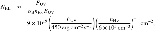$\begin{array}{ccc}{\mathit{N}}_{\mathrm{HII}}& \mathrm{\approx }& \frac{{\mathit{F}}_{\mathrm{UV}}}{{\mathit{\alpha }}_{\mathrm{B}}{\mathit{n}}_{\mathrm{H}\hspace{0.17em}\mathrm{◦}}{\mathit{E}}_{\mathrm{UV}}}\\ & \mathrm{=}& \mathrm{9}\mathrm{\times }{\mathrm{10}}^{\mathrm{19}}\left(\frac{{\mathit{F}}_{\mathrm{UV}}}{\mathrm{450}\hspace{0.17em}\mathrm{erg}\hspace{0.17em}\mathrm{c}{\mathrm{m}}^{-2}\hspace{0.17em}{\mathrm{s}}^{-1}}\right){\left(\frac{{\mathit{n}}_{\mathrm{H}\hspace{0.17em}\mathrm{◦}}}{\mathrm{6}\mathrm{\times }{\mathrm{10}}^{\mathrm{5}}\hspace{0.17em}{\mathrm{cm}}^{-3}}\right)}^{-1}\hspace{0.17em}{\mathrm{cm}}^{-2}\mathit{,}\end{array}$(38)where α_B ≃ 2.6 × 10^-13 cm³ s^-1 is the Case B recombination coefficient, and where (following Murray-Clay et al. 2009) we adopted a characteristic ionizing photon energy of E_UV = 20 eV. This estimate indicates that, even for a comparatively low ionizing flux, the entire planetary gas in the interaction region would be fully ionized, implying that this component would not be detectable in Lyα. A possible caveat to this conclusion may arise when the configuration is not in quasi-static equilibrium, and in particular if the ionization time, 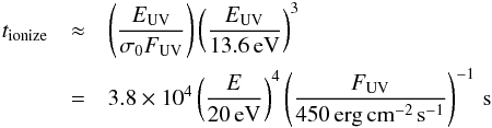$\begin{array}{ccc}{\mathit{t}}_{\mathrm{ionize}}& \mathrm{\approx }& \left(\frac{{\mathit{E}}_{\mathrm{UV}}}{{\mathit{\sigma }}_{\mathrm{0}}{\mathit{F}}_{\mathrm{UV}}}\right){\left(\frac{{\mathit{E}}_{\mathrm{UV}}}{\mathrm{13.6}\hspace{0.17em}\mathrm{eV}}\right)}^{\mathrm{3}}\\ & \mathrm{=}& \mathrm{3.8}\mathrm{\times }{\mathrm{10}}^{\mathrm{4}}{\left(\frac{\mathit{E}}{\mathrm{20}\hspace{0.17em}\mathrm{eV}}\right)}^{\mathrm{4}}{\left(\frac{{\mathit{F}}_{\mathrm{UV}}}{\mathrm{450}\hspace{0.17em}\mathrm{erg}\hspace{0.17em}\mathrm{c}{\mathrm{m}}^{-2}\hspace{0.17em}{\mathrm{s}}^{-1}}\right)}^{-1}\hspace{0.17em}\mathrm{s}\end{array}$(39)(where σ₀ ≃ 6 × 10^-18 cm² is the hydrogen photoionization cross section at the Lyman edge), is longer than the travel time of the planetary gas to the interaction region. However, this is probably not relevant to Type I configurations on account of the low velocity of the outflowing gas. The planetary gas in Type I systems might nevertheless be detectable in other absorption lines, such as the UV h and k resonance lines of Mg II.

Type II: R _t > R _w > R _m

Type II interactions occur when the planetary outflow is comparatively strong (corresponding to either a high irradiating flux or a small escape speed), so that the stellar plasma is intercepted by the planetary outflow (i.e., R_w>R_m). We again expect this plasma (which moves with a velocity of a few hundred km s^-1 with respect to the planet) to pass through a bow shock, and, after being shocked, to sweep back the planetary outflow into a tail. Because of the larger momentum flux in the planetary outflow in comparison with the Type I case, Type II tails are wider than their Type I counterparts for a given value of B_°. However, just as in the case of Type I interactions, the tail gas remains confined to the vicinity of the planet’s orbit, in this case because R_t>R_w. Its tilt angle (θ_tail) with respect to the orbit can be similarly estimated using Eq. (37).

Since in this case the planetary outflow is supercritical by the time it collides with the stellar plasma on the day side of the planet (at which point its speed v _w° is ≲30 km s^-1, on the order of v_{esc °}), it is also decelerated in a shock. The two shocks are separated by a contact discontinuity, across which the total (thermal + magnetic) pressure is the same. This, in turn, implies that the normal components (with respect to the contact discontinuity surface) of the ram pressures of the two flows are approximately equal in the frame of the contact discontinuity (which, in a steady state, is the same as that of the planet). As a rough estimate, we write 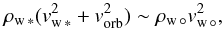${\mathit{\rho }}_{\mathrm{w}\hspace{0.17em}\mathrm{\ast }}\mathrm{(}{\mathit{v}}_{\mathrm{w}\hspace{0.17em}\mathrm{\ast }}^{\mathrm{2}}\mathrm{+}{\mathit{v}}_{\mathrm{orb}}^{\mathrm{2}}\mathrm{)}\mathrm{~}{\mathit{\rho }}_{\mathrm{w}\hspace{0.17em}\mathrm{◦}}{\mathit{v}}_{\mathrm{w}\hspace{0.17em}\mathrm{◦}}^{\mathrm{2}}\mathit{,}$(40)where, as we already noted, v_{w ∗} is typically on the order of v_orb for a hot Jupiter. The estimate (40) implies that the ratio of the preshock densities in the interaction region is ${\mathit{\rho }}_{\mathrm{w}\hspace{0.17em}\mathrm{\ast }}\mathit{/}{\mathit{\rho }}_{\mathrm{w}\hspace{0.17em}\mathrm{◦}}\mathrm{~}{\mathit{v}}_{\mathrm{w}\hspace{0.17em}\mathrm{◦}}^{\mathrm{2}}\mathit{/}\mathrm{(}{\mathit{v}}_{\mathrm{w}\hspace{0.17em}\mathrm{\ast }}^{\mathrm{2}}\mathrm{+}{\mathit{v}}_{\mathrm{orb}}^{\mathrm{2}}\mathrm{)}$, which for v_{w °} ~ 0.1 v_{w ∗} is ~0.01. The ratio of the corresponding postshock densities need not be the same on account of differences in the shock strength and the postshock cooling efficiency between the two winds, but it would likely still be ≪1. It also follows from Eq. (40) that the ratio of the mass inflow rates into the interaction zone, $\mathrm{~}{\mathit{\rho }}_{\mathrm{w}\hspace{0.17em}\mathrm{\ast }}\mathrm{(}{\mathit{v}}_{\mathrm{w}\hspace{0.17em}\mathrm{\ast }}^{\mathrm{2}}\mathrm{+}{\mathit{v}}_{\mathrm{orb}}^{\mathrm{2}}{\mathrm{)}}^{\mathrm{1}\mathit{/}\mathrm{2}}\mathit{/}\mathrm{(}{\mathit{\rho }}_{\mathrm{w}\hspace{0.17em}\mathrm{◦}}{\mathit{v}}_{\mathrm{w}\hspace{0.17em}\mathrm{◦}}\mathrm{)}$, is $\mathrm{~}{\mathit{v}}_{\mathrm{w}\hspace{0.17em}\mathrm{◦}}\mathit{/}\mathrm{(}{\mathit{v}}_{\mathrm{w}\hspace{0.17em}\mathrm{\ast }}^{\mathrm{2}}\mathrm{+}{\mathit{v}}_{\mathrm{orb}}^{\mathrm{2}}{\mathrm{)}}^{\mathrm{1}\mathit{/}\mathrm{2}}$ (~0.1 for our adopted values). This suggests that, as in the Type I case, the postshock density and column density in the interaction region is dominated by the planetary material. Although our simulations have not produced examples of a Type II interaction, we can use the simulation results for model FvRb (Fig. 9), which represents an example of a Type III interaction that involves a comparatively massive planetary outflow (see Table 2 and Sect. 4.3), to infer an upper bound of ~10^-16 g cm^-3 on the typical postshock planetary density in this case. We note in this connection that a supercritical planetary outflow is also shocked on the night side of the planet when it hits the gas that had been shocked farther upstream and subsequently dragged backward around the planet¹⁰. Moving farther out from the star in that direction, one again encounters unshocked stellar-wind gas that expands nearly radially, so the density there rapidly becomes very low.

Our estimate of the density of the planetary gas in the interaction region is two orders of magnitude larger in this case than the typical value we adopted for the Type I interaction (~10^-16 g cm^-3, associated with a high flux value, vs. ~10^-18 g cm^-3, which was obtained for a low UV flux). Using Eq. (38), we deduce a nominal ionized column of N_HII ≈ 10²¹ cm^-2 for these parameters, as compared with a total column of N_{H °} ≲ 8 × 10¹⁷, indicating that, in this case too, the interacting gas can be expected to be fully ionized if in equilibrium. The equilibrium assumption could be questioned since the gas is clearly in motion for Type II configurations; however, for the high flux value that characterizes the flow in model FvRb, the nominal ionization time inferred from Eq. (39) (a few tens of seconds) is much shorter than any relevant flow time. In addition, the shock heating of the planetary outflow can also contribute to the ionization of this gas¹¹. It is therefore likely that much of the gas that participates in a Type II interaction is ionized, although this conclusion needs to be checked explicitly for each given set of parameters.

Type III: R_w>R_m and R_w>R_t

Type III interactions are similar to those of Type II in that they involve a strong planetary wind (R_w>R_m). However, in this case the planetary outflow, after being stopped in a shock, is only partly swept back into a tail, with another part responding to the gravitational pull of the star (which is felt because R_w>R_t) and penetrating the stellar plasma ahead of the planet, forming a stream that spirals in and accretes onto the star¹².

The accretion stream exhibits a complex, fragmented morphology that arises from Kelvin-Helmholtz and Rayleigh-Taylor instabilities − triggered, respectively, by the tangential velocity shear and by the radial acceleration exerted by the stellar wind gas on the denser planetary material. The stellar gravity further contributes to the development of the latter instability on account of the “heavy on top of light” density stratification. These processes, and possibly also the magnetic stresses acting on the inflowing plasma, fragment the inspiraling stream, resulting in the formation of multiple accretion filaments that hit the stellar surface at different spots. The general location where the accretion stream impacts the stellar surface is determined by the stellar and planetary wind parameters and by the orbital distance of the planet, but it is typically well ahead of the instantaneous sub-planetary point (the phase difference being ~90° in the example shown in Fig. 9). We do not observe the formation of a circumstellar disk in our simulations, evidently because the drag exerted by the stellar outflow and the mixing between the two plasmas result in efficient removal of angular momentum from the inspiraling gas.

There have been several claims in the literature for enhanced activity on the host star – manifested in optical chromospheric emission lines (particularly Ca II), transition-region far-UV (FUV) emission lines (such as Si IV), and coronal X-ray emission – that might be attributable to an interaction with a close-in planet (e.g., Shkolnik et al. 2003, 2004, 2005, 2008; Walker et al. 2008; Pillitteri et al. 2010, 2011, 2014, 2015). The accretion streams produced in Type III interactions could potentially trigger such events. In particular, they may be associated with active regions that are inferred to lie significantly ahead of the sub-planetary point – as in HD 179949 and τ Boo, where a phase difference of ~70° was inferred from measurements of the Ca II K line (Shkolnik et al. 2008; Walker et al. 2008), and in HD 189733, where a lead phase of ~70°–90° was deduced from X-ray and FUV observations (Pillitteri et al. 2014, 2015). An alternative interpretation of these phenomena that has been discussed in the literature involves a direct magnetic interaction of the type observed in planetary moons (such as Io) in the solar system. We note, however, that in their simplest form, such interactions are unlikely to exhibit a significant phase shift. Furthermore, the energy flux generated in such an interaction in a source like HD 179499 is calculated (Saur et al. 2013) to be over two orders of magnitude lower than the observationally inferred value (Shkolnik et al. 2005). More generally, the star–planet interactions in the case of hot Jupiters involve higher orbital speeds and denser plasmas, which are not conducive to the establishment of a direct magnetic linkage between the two bodies as in the Io–Jupiter system.

Type IV: R_m>R_w and R_m>R_t

This case is analogous to the Type III one in that the interaction region lies outside the planet’s Hill radius, resulting in the accretion of planetary gas onto the stellar surface. However, just as a Type III interaction could be regarded as a special case of a Type II one, with both involving a strong planetary outflow, a Type IV interaction also bears similarity to a Type-I interaction in having a comparatively weak planetary wind (R_m>R_w). In this case the planetary magnetosphere, which is loaded by the subsonic gas evaporated by the stellar radiation field, intercepts the stellar plasma beyond the L₁ point, where the stellar gravity is the dominant force acting on the planetary gas. This situation resembles the classic Roche-lobe overflow picture, although both the planetary magnetic field and the outflowing, magnetized stellar plasma also play a role in shaping the accretion flow morphology. In particular, when the orbital radius is small enough, the relative motion between the stellar gas and the planet may be supercritical and therefore lead to the formation of a bow shock ahead of the planet, as in the Type I case, even as mass transfer from the planet to the star takes place in the vicinity of the substellar region. However, no bow shock forms on the star-facing side in our “near” models because the stellar magnetic field (and hence the Alfvén speed) at R_m is large enough in these cases to keep the relative motion between the stellar gas and the planet subcritical (see Fig. 12).

The structure of the accretion flow and its dynamical implications are similar in this case to the situation in Type III interactions. In particular, the flow can fragment into separate accretion filaments, especially when the orbital separation is large. However, because of the absence of a strong planetary outflow in the Type IV case, the accretion stream does not exhibit the spiral structure observed in Type III interactions and instead maintains an approximately linear shape. In this case the flow typically hits the stellar surface near the sub-planetary point, the more so the closer the planet is to the star. This type of interaction may thus be relevant to the interpretation of enhanced stellar chromospheric/X-ray activity that is inferred to occur near the sub-planetary point (and could provide an alternative to the “direct magnetic interaction” scenario also in this case).

A Roche-lobe overflow model was previously proposed for the interpretation of early ingress indications in UV absorption-line observations of the short-period (R_orb = 0.023 AU) hot Jupiter WASP-12b (Fossati et al. 2010). In particular, Lai et al. (2010), considered the possible contributions of an accretion stream and of an inner accretion disk, and also speculated on absorption in the interaction region between a stellar wind and the planetary magnetosphere. They did not, however, include the effect of the stellar radiation heating of the planet and the influence of the stellar plasma on the accretion stream. Bisikalo et al. (2013) carried out a hydrodynamical simulation and drew attention to the interaction between the accretion stream and the stellar outflow, but they did not consider the effect of a stellar and/or a planetary magnetic field. The results presented in this paper provide a more general framework for modeling systems like WASP-12, and may also aid in modeling other types of close-in planets where Roche-lobe overflow could play a role (e.g., Valsecchi et al. 2014).

4.3. Classification of the simulations

The application of our proposed classification scheme to the models that we have simulated is presented in Table 3. We note that Type II interactions are not represented in this table. This interaction is intermediate between the Type I and Type III cases – for which we do have examples – in that the planetary outflow must be strong enough to cause R_w to exceed R_m but not so strong that it will also exceed R_t. Computational constraints prevented us from exploring a wider parameter space that would have encompassed this interaction.

5. Summary and conclusions

In this paper we study the different types of star-planet interactions that can occur in systems harboring hot Jupiters. We perform a series of parametrized 3D MHD numerical simulations, incorporating the star, the planet, and consistent stellar and planetary winds. Based on the results of a grid of models, we propose a classification of the interactions into four general categories (which we label I–IV; see Fig. 13). We describe in detail the dynamical features exhibited in each case, and provide expressions for the three characteristic length scales that underlie our classification scheme in terms of the system’s physical parameters. We also briefly discuss general characteristics of these interactions that could have a bearing on their observational properties.

The main conclusions of our analysis can be summarized as follows:

• 1.

  Except very close to the star, where the stellar magnetic field(and the associated Alfvén speed) might be large enough to renderthe flow subcritical, the stellar outflow intercepted by the planet isstopped in a bow shock. The shock forms even when the stellarwind is not yet fully accelerated because of the high (≳100 km s^-1) azimuthal velocity component of the stellar gas in the planet’s frame.

• 2.

  In Type I interactions, the stellar plasma is intercepted by the planetary magnetosphere, which, in turn, is swept back into a plasma tail that is blown away by the stellar wind.

• 3.

  In interactions of Type II and III, the stellar plasma is intercepted by a strong planetary outflow that opens up the magnetosphere. The shocked planetary plasma is dragged backward by the stellar outflow, forming a wide tail that is fragmented by dynamical instabilities. In the Type II case, the shocked planetary plasma lies inside the Roche lobe and remains confined to the vicinity of the orbital radius. In contrast, in the Type III case the interaction occurs outside the Roche surface, resulting in part of the shocked planetary plasma forming an accretion stream that spirals toward the star until it impacts the stellar surface. The dynamical interaction of this stream with the magnetized stellar wind enables this gas to lose energy and angular momentum and fall in, instead of forming a plasma torus. The stream is also subject to dynamical instabilities, which cause it to split into multiple accretion filaments that hit the stellar surface at different spots.

• 4.

  In Type IV interactions the stellar outflow is intercepted by the planetary magnetic field outside the Roche radius. This situation resembles a classic Roche-lobe overflow, although it differs in detail on account of the presence of the planetary magnetic field and of the magnetized stellar outflow. In contrast with the Type III accretion stream, which reaches the stellar surface well ahead of the sub-planetary point, in this case the planetary gas falls in nearly radially.

• 5.

  In general, the density and column density in the interaction region are dominated by the planetary gas. Typically, this gas can be expected to be fully ionized, implying that detection through absorption features of neutral species such as H I and Mg I is unlikely.

Acknowledgments

We thank Sean Matt for his helpful guidance in the implementation of the stellar wind models. T.M. is grateful for the hospitality and support of the Harvard-Smithsonian Center for Astrophysics, and for the very useful input from I. Pillitteri and S. Wolk. We also acknowledge the constructive comments of the anonymous referee. This work was completed with resources provided by the University of Chicago Research Computing Center and was supported in part by NASA ATP grant NNX13AH56G and NSF grant AST-0908184.

References

All Tables

All Figures

	Fig. 1 Logarithmic density contours, field lines (solid lines), and poloidal Alfvén surface (dashed line) in the final steady state of the 3D stellar wind model employed in this paper (left panel) and of a 2.5D high-resolution simulation (right panel).
In the text

	Fig. 2 Logarithmic density (left) and radial velocity (right) in the final steady state of the 3D stellar wind model as a function of the distance R from the center of the star along the equatorial (x) and axial (z) directions (solid and dashed lines, respectively).
In the text

Fig. 3 Logarithmic density (left) and radial velocity (right) as a function of distance from the planet’s center for the isotropic outflow model used to initialize the 3D wind simulation for a “light” hot Jupiter (M° = 0.5 MJ, R° = 1.5 RJ). The symbols “+” and “×” denote, respectively, the high- and low-flux cases (modeled with T° = 104 K and T° = 6 × 103 K, respectively). The solid and dashed lines are from the corresponding 1D simulations that take into account the relevant heating and cooling processes (see text for details).

In the text

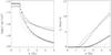	Fig. 4 Same as Fig. 3, but for a Jupiter-like planet (M° = MJ, R° = RJ).
In the text

Fig. 5 Initial conditions in the lab frame for model FVRB. The axes are in units of 0.01 AU. Logarithmic density contours (in units of g cm-3) are shown in the x-y plane (z = 0; left panel) and in the x-z plane (y = 0; right panels). The top right panel is focused on the star and the bottom right on the planet. Solid lines represent the magnetic field, arrows show the velocity field (with the longest one corresponding to ~290 km s-1), dashed lines the poloidal Alfvén surface (${\mathit{v}}_{\mathit{x}}^{\mathrm{2}}\mathrm{+}{\mathit{v}}_{\mathit{z}}^{\mathrm{2}}\mathrm{=}\mathrm{(}{\mathit{B}}_{\mathit{x}}^{\mathrm{2}}\mathrm{+}{\mathit{B}}_{\mathit{z}}^{\mathrm{2}}\mathrm{)}\mathit{/}\mathrm{4}\mathit{\pi \rho }$), and dotted lines the poloidal sonic surface (${\mathit{v}}_{\mathit{x}}^{\mathrm{2}}\mathrm{+}{\mathit{v}}_{\mathit{z}}^{\mathrm{2}}\mathrm{=}\mathit{\gamma P}\mathit{/}\mathit{\rho }$). The cross in the bottom right panel denotes the location of the L1 point.

In the text

Fig. 6 Logarthimic density (color contours in units of g cm-3), velocity (arrows), magnetic field (solid lines), critical surfaces (dotted line: sonic, dashed line: Alfvén), and the L1 point (cross) for the final steady state of model fvRb. Distances are measured in units of 0.01 AU. The panels are arranged as in Fig. 5, with the left and top right panels centered on the star, and the bottom right one on the planet.

In the text

	Fig. 7 Same as the left panel of Fig. 6, but for models fvRB (left) and FVRb (right).
In the text

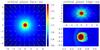	Fig. 8 Same as Fig. 6, but for model fVRb.
In the text

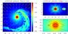	Fig. 9 Same as Fig. 6, but for model FvRb.
In the text

	Fig. 10 3D representation of the density structure and of the magnetic field lines (blue: stellar; red: planetary) for model FvRb. The logarithmic density scale is chosen for visualization purposes and does not correspond to that of Fig. 9.
In the text

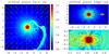	Fig. 11 Same as Fig. 6, but for model FVRB.
In the text

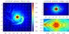	Fig. 12 Same as Fig. 6, but for model FvrB.
In the text

Fig. 13 Schematic of the different possible star–planet interactions, showing face-on views in the orbital plane of the four distinct morphological structures (denoted by the Latin numerals I, II, III, and IV) as they appear in the planet’s frame. The large and small solid disks (on the left and right sides of each panel) represent the star and the hot Jupiter, respectively, the shaded areas highlight material that flowed out of the planet, the arrows indicate gas motions, and the closed loops sketch the planetary magnetosphere. The solid circular arcs in panels I and IV have a radius Rm, the distance where the magnetospheric pressure equals the total ambient pressure, whereas the dashed circular arcs in panels II and III mark the distance Rw where the ambient pressure equals the ram pressure of the planetary wind. The dotted line indicates the contour of the effective (gravity plus centrifugal) potential that passes through the Lagrange point L1 (at a distance Rt from the planet). The proposed classification scheme is based on the relative ordering of Rm, Rw, and Rt.

In the text

References

- Adams, F. C. 2011, ApJ, 730, 27 [NASA ADS] [CrossRef] [Google Scholar]
- Bean, J. L., Désert, J.-M., Seifahrt, A., et al. 2013, ApJ, 771, 108 [NASA ADS] [CrossRef] [Google Scholar]
- Ben-Jaffel, L. 2007, ApJ, 671, L61 [NASA ADS] [CrossRef] [Google Scholar]
- Ben-Jaffel, L. 2008, ApJ, 688, 1352 [NASA ADS] [CrossRef] [Google Scholar]
- Ben-Jaffel, L., & Ballester, G. E. 2013, A&A, 553, A52 [NASA ADS] [CrossRef] [EDP Sciences] [Google Scholar]
- Bisikalo, D., Kaygorodov, P., Ionov, D., et al. 2013, ApJ, 764, 19 [NASA ADS] [CrossRef] [Google Scholar]
- Bourrier, V., & Lecavelier des Etangs, A. 2013, A&A, 557, A124 [NASA ADS] [CrossRef] [EDP Sciences] [Google Scholar]
- Bourrier, V., Lecavelier des Etangs, A., Dupuy, H., et al. 2013, A&A, 551, A63 [NASA ADS] [CrossRef] [EDP Sciences] [Google Scholar]
- Bourrier, V., Lecavelier des Etangs, A., & Vidal-Madjar, A. 2014, A&A, 565, A105 [NASA ADS] [CrossRef] [EDP Sciences] [Google Scholar]
- Burrows, A., Guillot, T., Hubbard, W. B., et al. 2000, ApJ, 534, L97 [NASA ADS] [CrossRef] [PubMed] [Google Scholar]
- Buzasi, D. 2013, ApJ, 765, L25 [NASA ADS] [CrossRef] [Google Scholar]
- Cohen, O., & Drake, J. J. 2014, ApJ, 783, 55 [NASA ADS] [CrossRef] [Google Scholar]
- Cohen, O., Drake, J. J., Kashyap, V. L., et al. 2009, ApJ, 704, L85 [NASA ADS] [CrossRef] [Google Scholar]
- Cohen, O., Drake, J. J., Kashyap, V. L., Sokolov, I. V., & Gombosi, T. I. 2010, ApJ, 723, L64 [NASA ADS] [CrossRef] [Google Scholar]
- Cohen, O., Kashyap, V. L., Drake, J. J., et al. 2011a, ApJ, 733, 67 [NASA ADS] [CrossRef] [Google Scholar]
- Cohen, O., Kashyap, V. L., Drake, J. J., Sokolov, I. V., & Gombosi, T. I. 2011b, ApJ, 738, 166 [NASA ADS] [CrossRef] [Google Scholar]
- Cohen, O., Drake, J. J., Glocer, A., et al. 2014, ApJ, 790, 57 [NASA ADS] [CrossRef] [Google Scholar]
- Cranmer, S. R., van Ballegooijen, A. A., & Edgar, R. J. 2007, ApJS, 171, 520 [Google Scholar]
- Ehrenreich, D., Lecavelier Des Etangs, A., Hébrard, G., et al. 2008, A&A, 483, 933 [NASA ADS] [CrossRef] [EDP Sciences] [Google Scholar]
- Fabrycky, D. C., & Winn, J. N. 2009, ApJ, 696, 1230 [NASA ADS] [CrossRef] [Google Scholar]
- Fossati, L., Haswell, C. A., Froning, C. S., et al. 2010, ApJ, 714, L222 [NASA ADS] [CrossRef] [Google Scholar]
- García Muñoz, A. 2007, Planet. Space Sci., 55, 1426 [NASA ADS] [CrossRef] [Google Scholar]
- Koskinen, T. T., Harris, M. J., Yelle, R. V., & Lavvas, P. 2013, Icarus, 226, 1678 [Google Scholar]
- Kulow, J. R., France, K., Linsky, J., & Loyd, R. O. P. 2014, ApJ, 786, 132 [NASA ADS] [CrossRef] [Google Scholar]
- Lai, D., Helling, C., & van den Heuvel, E. P. J. 2010, ApJ, 721, 923 [NASA ADS] [CrossRef] [Google Scholar]
- Laine, R. O., Lin, D. N. C., & Dong, S. 2008, ApJ, 685, 521 [NASA ADS] [CrossRef] [Google Scholar]
- Lanza, A. F. 2008, A&A, 487, 1163 [NASA ADS] [CrossRef] [EDP Sciences] [Google Scholar]
- Lanza, A. F. 2009, A&A, 505, 339 [NASA ADS] [CrossRef] [EDP Sciences] [Google Scholar]
- Lanza, A. F. 2013, A&A, 557, A31 [NASA ADS] [CrossRef] [EDP Sciences] [Google Scholar]
- Lecavelier des Etangs, A., Vidal-Madjar, A., McConnell, J. C., & Hébrard, G. 2004, A&A, 418, L1 [NASA ADS] [CrossRef] [EDP Sciences] [Google Scholar]
- Lecavelier des Etangs, A., Ehrenreich, D., Vidal-Madjar, A., et al. 2010, A&A, 514, A72 [NASA ADS] [CrossRef] [EDP Sciences] [Google Scholar]
- Lecavelier des Etangs, A., Bourrier, V., Wheatley, P. J., et al. 2012, A&A, 543, L4 [NASA ADS] [CrossRef] [EDP Sciences] [Google Scholar]
- Llama, J., Wood, K., Jardine, M., et al. 2011, MNRAS, 416, L41 [NASA ADS] [CrossRef] [Google Scholar]
- Llama, J., Vidotto, A. A., Jardine, M., et al. 2013, MNRAS, 436, 2179 [NASA ADS] [CrossRef] [Google Scholar]
- Matsumura, S., Peale, S. J., & Rasio, F. A. 2010, ApJ, 725, 1995 [NASA ADS] [CrossRef] [Google Scholar]
- Matt, S., & Balick, B. 2004, ApJ, 615, 921 [NASA ADS] [CrossRef] [Google Scholar]
- Matt, S., & Pudritz, R. E. 2008, ApJ, 678, 1109 [Google Scholar]
- Matt, S. P., MacGregor, K. B., Pinsonneault, M. H., & Greene, T. P. 2012a, ApJ, 754, L26 [NASA ADS] [CrossRef] [Google Scholar]
- Matt, S. P., Pinzón, G., Greene, T. P., & Pudritz, R. E. 2012b, ApJ, 745, 101 [NASA ADS] [CrossRef] [Google Scholar]
- Mignone, A., Bodo, G., Massaglia, S., et al. 2007, ApJS, 170, 228 [Google Scholar]
- Mignone, A., Zanni, C., Tzeferacos, P., et al. 2012, ApJS, 198, 7 [Google Scholar]
- Mura, A., Wurz, P., Schneider, J., et al. 2011, Icarus, 211, 1 [NASA ADS] [CrossRef] [Google Scholar]
- Murray-Clay, R. A., Chiang, E. I., & Murray, N. 2009, ApJ, 693, 23 [Google Scholar]
- Ness, N. F. 1965, J. Geophys. Res., 70, 2989 [NASA ADS] [CrossRef] [Google Scholar]
- Owen, J. E., & Adams, F. C. 2014, MNRAS, 444, 3761 [NASA ADS] [CrossRef] [Google Scholar]
- Owen, J. E., & Jackson, A. P. 2012, MNRAS, 425, 2931 [NASA ADS] [CrossRef] [Google Scholar]
- Parker, E. N. 1958, ApJ, 128, 664 [Google Scholar]
- Parker, E. N. 1960, ApJ, 132, 821 [NASA ADS] [CrossRef] [Google Scholar]
- Pillitteri, I., Wolk, S. J., Cohen, O., et al. 2010, ApJ, 722, 1216 [NASA ADS] [CrossRef] [Google Scholar]
- Pillitteri, I., Günther, H. M., Wolk, S. J., Kashyap, V. L., & Cohen, O. 2011, ApJ, 741, L18 [NASA ADS] [CrossRef] [Google Scholar]
- Pillitteri, I., Wolk, S. J., Lopez-Santiago, J., et al. 2014, ApJ, 785, 145 [NASA ADS] [CrossRef] [Google Scholar]
- Pillitteri, I., Maggio, A., Micela, G., et al. 2015, ApJ, in press [arXiv:1503.05590] [Google Scholar]
- Rappaport, S., Levine, A., Chiang, E., et al. 2012, ApJ, 752, 1 [NASA ADS] [CrossRef] [Google Scholar]
- Rappaport, S., Barclay, T., DeVore, J., et al. 2014, ApJ, 784, 40 [NASA ADS] [CrossRef] [Google Scholar]
- Ribas, I., Guinan, E. F., Güdel, M., & Audard, M. 2005, ApJ, 622, 680 [NASA ADS] [CrossRef] [Google Scholar]
- Saur, J., Grambusch, T., Duling, S., Neubauer, F. M., & Simon, S. 2013, A&A, 552, A119 [NASA ADS] [CrossRef] [EDP Sciences] [Google Scholar]
- Schneider, J., Rauer, H., Lasota, J. P., Bonazzola, S., & Chassefiere, E. 1998, in Brown Dwarfs and Extrasolar Planets, eds. R. Rebolo, E. L. Martin, & M. R. Zapatero Osorio, ASP Conf. Ser., 134, 241 [Google Scholar]
- Seager, S. 2011, Exoplanets atmospheres: A theoretical outlook, IAU Symp., 276, 198 [NASA ADS] [Google Scholar]
- Shkolnik, E., Walker, G. A. H., & Bohlender, D. A. 2003, ApJ, 597, 1092 [NASA ADS] [CrossRef] [Google Scholar]
- Shkolnik, E., Walker, G. A. H., & Bohlender, D. A. 2004, ApJ, 609, 1197 [NASA ADS] [CrossRef] [Google Scholar]
- Shkolnik, E., Walker, G. A. H., Bohlender, D. A., Gu, P.-G., & Kürster, M. 2005, ApJ, 622, 1075 [NASA ADS] [CrossRef] [Google Scholar]
- Shkolnik, E., Bohlender, D. A., Walker, G. A. H., & Collier Cameron, A. 2008, ApJ, 676, 628 [NASA ADS] [CrossRef] [Google Scholar]
- Spitzer, L. 1978, J. Roy. Astron. Soc. Can., 72, 349 [Google Scholar]
- Strugarek, A., Brun, A. S., Matt, S. P., & Réville, V. 2014, ApJ, 795, 86 [NASA ADS] [CrossRef] [Google Scholar]
- Teşileanu, O., Mignone, A., & Massaglia, S. 2008, A&A, 488, 429 [NASA ADS] [CrossRef] [EDP Sciences] [Google Scholar]
- Tian, F., Toon, O. B., Pavlov, A. A., & De Sterck, H. 2005, ApJ, 621, 1049 [NASA ADS] [CrossRef] [Google Scholar]
- Trammell, G. B., Arras, P., & Li, Z.-Y. 2011, ApJ, 728, 152 [NASA ADS] [CrossRef] [Google Scholar]
- Trammell, G. B., Li, Z.-Y., & Arras, P. 2014, ApJ, 788, 161 [NASA ADS] [CrossRef] [Google Scholar]
- Tremblin, P., & Chiang, E. 2013, MNRAS, 428, 2565 [NASA ADS] [CrossRef] [Google Scholar]
- Valsecchi, F., Rasio, F. A., & Steffen, J. H. 2014, ApJ, 793, L3 [NASA ADS] [CrossRef] [Google Scholar]
- Vidal-Madjar, A., Désert, J.-M., Lecavelier des Etangs, A., et al. 2004, ApJ, 604, L69 [NASA ADS] [CrossRef] [Google Scholar]
- Vidotto, A. A., Jardine, M., & Helling, C. 2010, ApJ, 722, L168 [NASA ADS] [CrossRef] [Google Scholar]
- Vidotto, A. A., Jardine, M., & Helling, C. 2011a, MNRAS, 411, L46 [NASA ADS] [CrossRef] [Google Scholar]
- Vidotto, A. A., Jardine, M., & Helling, C. 2011b, MNRAS, 414, 1573 [NASA ADS] [CrossRef] [Google Scholar]
- Vidotto, A. A., Jardine, M., Morin, J., et al. 2014, MNRAS, 438, 1162 [NASA ADS] [CrossRef] [Google Scholar]
- Walker, G. A. H., Croll, B., Matthews, J. M., et al. 2008, A&A, 482, 691 [NASA ADS] [CrossRef] [EDP Sciences] [Google Scholar]
- Yelle, R. V. 2004, Icarus, 170, 167 [NASA ADS] [CrossRef] [Google Scholar]
- Yelle, R. V. 2006, Icarus, 183, 508 [NASA ADS] [CrossRef] [Google Scholar]