| Issue |
A&A
Volume 578, June 2015
|
|
|---|---|---|
| Article Number | A60 | |
| Number of page(s) | 14 | |
| Section | The Sun | |
| DOI | https://doi.org/10.1051/0004-6361/201425468 | |
| Published online | 04 June 2015 | |
Energy and energy flux in axisymmetric slow and fast waves⋆
1 Centre for mathematical Plasma Astrophysics, Mathematics Department, KU Leuven, Celestijnenlaan 200B bus 2400, 3001 Leuven, Belgium
e-mail: This email address is being protected from spambots. You need JavaScript enabled to view it.
; This email address is being protected from spambots. You need JavaScript enabled to view it.
2 Astrophysics Research Centre, School of Mathematics and Physics, Queens University Belfast, Belfast BT7 1NN, UK
Received: 5 December 2014
Accepted: 9 April 2015
Abstract
Aims. We aim to calculate the kinetic, magnetic, thermal, and total energy densities and the flux of energy in axisymmetric sausage modes. The resulting equations should contain as few parameters as possible to facilitate applicability for different observations.
Methods. The background equilibrium is a one-dimensional cylindrical flux tube model with a piecewise constant radial density profile. This enables us to use linearised magnetohydrodynamic equations to calculate the energy densities and the flux of energy for axisymmetric sausage modes.
Results. The equations used to calculate the energy densities and the flux of energy in axisymmetric sausage modes depend on the radius of the flux tube, the equilibrium sound and Alfvén speeds, the density of the plasma, the period and phase speed of the wave, and the radial or longitudinal components of the Lagrangian displacement at the flux tube boundary. Approximate relations for limiting cases of propagating slow and fast sausage modes are also obtained. We also obtained the dispersive first-order correction term to the phase speed for both the fundamental slow body mode under coronal conditions and the slow surface mode under photospheric conditions.
Key words: magnetohydrodynamics (MHD) / methods: analytical / Sun: atmosphere / Sun: oscillations
Appendix A is available in electronic form at http://www.aanda.org
© ESO, 2015
1. Introduction
The solar atmosphere is a dynamic, magnetised plasma containing numerous distinct structures from active regions to coronal loops. These structures have been observed to support different oscillatory magnetohydrodynamic (MHD) modes (for recent reviews see Banerjee et al. 2007; De Moortel 2009; De Moortel & Nakariakov 2012). Magnetohydrodynamic waves are important for several reasons. First, they can be used to calculate the important background plasma parameters using MHD seismology of the solar atmosphere (e.g. Andries et al. 2005, 2009; Banerjee et al. 2007; De Moortel & Nakariakov 2012). Second, because MHD waves can carry energy over large distances, it has historically been thought that they can play a major role in the heating of the corona. Extensive discussions on coronal heating can be found in Walsh & Ireland (2003), Erdélyi (2004), Ofman (2005), and numerous others. To quantify the contribution of MHD waves to coronal heating we need both observations of MHD waves and methods to estimate the energy of those waves.
There have been many observations of MHD waves in different layers of the solar atmosphere with different instruments. In coronal loops MHD waves were observed with the Extreme ultraviolet Imaging Telescope (EIT) aboard the Solar and Heliospheric Observatory (SOHO; e.g. Thompson et al. 1999), with the Coronal Multi-Channel Polarimeter (CoMP; e.g. Tomczyk et al. 2007), with the extreme ultraviolet imaging spectrometer (EIS) aboard Hinode (e.g. Van Doorsselaere et al. 2008; Banerjee et al. 2009), and with the Solar Dynamics Observatory Atmospheric Imaging Assembly (SDO/AIA; e.g. Aschwanden & Schrijver 2011; Morton et al. 2012b) to give but a few examples. In the chromosphere, MHD waves have been detected using the Solar Optical Telescope (SOT) aboard Hinode (De Pontieu et al. 2007), using the Swedish Solar Telescope (SST, e.g. Jess et al. 2009), and using the Rapid Oscillations in the Solar Atmosphere (ROSA, Jess et al. 2010) instrument (e.g. Morton et al. 2011). In sunspots MHD waves have been observed for quite a long time (e.g. Bhatnagar 1971; Beckers & Schultz 1972; Jess et al. 2013). More recently, MHD waves have also been observed in smaller magnetic pores in the photosphere (e.g. Dorotovič et al. 2008, 2014; Yuan et al. 2014; Moreels et al. 2015). This non-exhaustive list of observations shows that there is a need for energy quantification methods in order to understand the energy supply of compressive MHD waves to the higher layers of the solar atmosphere. In these layers the wave energy is crucial to understanding the coronal heating problem.
There have been several papers that have estimated the energy in transverse kink oscillations. Morton et al. (2014) have used the ubiquity of propagating kink mode observations in the chromosphere to estimate the energy content of the observed kink waves. Thurgood et al. (2014) have detected transverse motions in solar plumes and used the displacement to estimate the energy in these transverse motions. Determining the energy of transverse kink motions has also received theoretical attention. Goossens et al. (2013a) used MHD theory to derive formulas that determine the energy of kink waves in the solar corona. Van Doorsselaere et al. (2014) have expanded on this idea and used MHD theory to write an expression for energy flux in terms of density filling factors.
In this paper we focus on axisymmetric slow and fast sausage modes, which have recently been discovered in numerous structures, but have not been adequately modelled to estimate their energy content. They have been detected in coronal loops (De Moortel et al. 2000; Wang et al. 2002, 2003; Krishna Prasad et al. 2012), in photospheric pores (Dorotovič et al. 2008, 2014; Morton et al. 2011; Moreels et al. 2015), in network bright points (McAteer et al. 2003; Bharti et al. 2006; Martínez González et al. 2011), in flares (Nakariakov et al. 2003; Melnikov et al. 2005; Van Doorsselaere et al. 2011), and in the chromosphere (Morton et al. 2012a). Some authors have attempted to estimate the amount of energy present in these observations. Morton et al. (2012a) have observed both sausage and kink modes in the chromosphere and used MHD theory to estimate the energy in the waves. They found that the energy of compressive (sausage) waves was higher than the energy in transverse waves. We believe that the approach used in Morton et al. (2012a) can be improved in several ways. First, the integration of the wave energy should be performed over the entire cylinder since the eigenfunctions change with radial position. Second, the energy outside the flux tube should also be calculated since this can be of the same order of magnitude as the internal energy.
In this work we calculate the wave energy in sausage modes using a similar approach to that presented by Goossens et al. (2013a). The aim is to calculate the energy using only the background plasma equilibrium parameters and the phase speed of the wave. In this way the formulas can easily be applied to different observations to estimate the energy of sausage modes. This is a very important aspect since it means that energetics can be determined at height-localised regions of the solar atmosphere. In combination with the data analysis method described in Moreels et al. (2015) we do not need multiwavelength imaging approaches to determine the phase speed of the wave. Therefore, we are able to determine the energy in sausage oscillations for single filter measurements.
The paper is organised as follows: Sect. 2 gives the mathematical framework; Sect. 3 describes some limiting cases for the energy calculation which are of physical interest, i.e. slow sausage modes in coronal loops (Sect. 3.1 and Appendix A) and fast sausage modes in coronal loops (Sect. 3.2); Sect. 4 lists the conclusions of this paper.
2. Mathematical framework
The mathematical framework in which the energy for sausage waves is calculated is split into three sections. Section 2.1 derives general energy equations which can be used for different waves modes in different atmospheres. In Sect. 2.2 we calculate the energy inside the flux tube for surface modes. Section 2.3 lists the energy equations for both the energy inside the flux tube for body modes and the energy outside the flux tube.
2.1. General energy equations
Our equilibrium model is a straight cylinder with a constant radius R where the plasma is uniform both inside and outside the cylinder with a possible jump at the boundary (see Edwin & Roberts 1983). The magnetic field is directed along the axis of the flux tube and is given by B0,i inside the flux tube and B0,e outside the flux tube. The plasma pressure and density are p0,i and ρ0,i inside the flux tube and p0,e and ρ0,e outside the flux tube. We assume that the plasma has no background flow, i.e. the equilibrium velocity is v0 = 0 both inside and outside the flux tube (see Fig. 1).
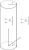 |
Fig. 1 Equilibrium configuration of the flux tube. |
Before starting the energy calculations it is instructive to first consider the limitations of this equilibrium model. The straight uniform flux tube model neglects several physical effects, e.g. density stratification, flux tube expansion, and flux tube curvature. These effects can be important depending on the solar structure under consideration. The density stratification combined with the flux tube expansion is very important in the photosphere/chromosphere region. However, while the uniform flux tube model neglects these effects it is still valid when used as a first-order approximation. Andries & Cally (2011) have shown that for a slowly expanding flux tube the perpendicular eigenfunctions of MHD waves remain very similar and are still in terms of Bessel functions. In the corona the density stratification and flux tube expansion are minimal, but the curvature of the flux tubes can be a significant effect. Although Van Doorsselaere et al. (2004b) have shown that the curvature has no effect on eigenfrequencies of kink modes for a particular density profile, Verwichte et al. (2006) have shown that curvature could result in leaky wave modes, especially for thick flux tubes. While the leaky nature of the MHD waves will drastically change the energy outside the flux tube it will have a minimal impact on the energy inside the flux tube assuming that the internal remaining energy only decreases slowly over one period of the wave. Therefore, the uniform flux tube model results for the energy inside the flux tube are still very useful for estimating the energy content inside the flux tube of slowly leaking MHD waves.
Zaitsev & Stepanov (1975), Edwin & Roberts (1983), Sakurai et al. (1991), and many others have solved the ideal MHD equations for this equilibrium configuration. The solution method uses the following steps. First, the ideal MHD equations are linearised around the equilibrium state, e.g.  where ρ0 is the background and
  is the small perturbation. From now on we drop the ϕ dependence since we are studying axisymmetric wave modes. Second, the resulting equations are solved analytically by performing a Fourier analysis in the ignorable coordinates, e.g. the density perturbation inside the flux tube can be written as
 ![Mathematical equation: \hbox{$\widetilde{\rho}(r,z,t) = \rho'(r)\exp\left[{\rm i}(kz-\omega t)\right]$}](/articles/aa/full_html/2015/06/aa25468-14/aa25468-14-eq13.png) . In this way all perturbed quantities can be related with the radial component of the Lagrangian displacement ξr and the total Eulerian pressure perturbation P′. Before listing the most important equations we would like to make the distinction between Eulerian and Lagrangian variables. This distinction can be easily explained from an observational point of view. We assume that we have a series of intensity images of the sun. When looking at a fixed set of pixels for all images we are using the Eulerian intensity. On the other hand, a magnetic structure can be used to define a set of pixels for each image that describe the structure, i.e. the set of pixels can change at each image. Defining the intensity based on this set of pixels means using the Lagrangian intensity. More information on the difference between Eulerian and Lagrangian variables can be found in Moreels et al. (2013).
. In this way all perturbed quantities can be related with the radial component of the Lagrangian displacement ξr and the total Eulerian pressure perturbation P′. Before listing the most important equations we would like to make the distinction between Eulerian and Lagrangian variables. This distinction can be easily explained from an observational point of view. We assume that we have a series of intensity images of the sun. When looking at a fixed set of pixels for all images we are using the Eulerian intensity. On the other hand, a magnetic structure can be used to define a set of pixels for each image that describe the structure, i.e. the set of pixels can change at each image. Defining the intensity based on this set of pixels means using the Lagrangian intensity. More information on the difference between Eulerian and Lagrangian variables can be found in Moreels et al. (2013).
Summarizing the most important equations, we have 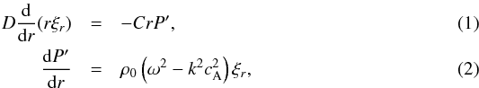 where C and D are given by
  In the above equations we have used the Alfvén speed cA, the sound speed cs, and the tube speed
  . The above equations are valid both inside and outside the flux tube. Equations (1)and (2)can be combined to form an ordinary differential equation for the total Eulerian pressure perturbation P′, which is solvable in terms of Bessel functions. Other useful equations are
 ![Mathematical equation: \begin{eqnarray} \xi_z&=&\frac{{\rm i}kc_{\mathrm{s}}^2}{\rho_0\left(c_{\mathrm{s}}^2+c_{\mathrm{A}}^2\right)\left(\omega^2-k^2c_{\mathrm{T}}^2\right)}P', \nonumber\\[1mm] \xi_\varphi &=& 0, \nonumber\\[1mm] \vec{B}'&=&{\rm i}kB_0\vec{\xi}-B_0\left(\nabla\cdot\vec{\xi}\right){\vec1_{\it z}}, \nonumber\\[1mm] p'&=&-\rho_0 c_{\mathrm{s}}^2\nabla\cdot\vec{\xi}, \nonumber\\[1mm] \nabla\cdot\vec{\xi}&=&\frac{-\omega^2}{\rho_0\left(c_{\mathrm{s}}^2+c_{\mathrm{A}}^2\right)\left(\omega^2-k^2c_{\mathrm{T}}^2\right)}P', \nonumber\\[1mm] \vec{E'}&=&{\rm i}\omega B_0\xi_r\vec{1_\varphi}\label{eq:MHD_pert}. \end{eqnarray}](/articles/aa/full_html/2015/06/aa25468-14/aa25468-14-eq23.png) (3)Equations (3)provide algebraic expressions for the perturbed quantities ξz, ξϕ, B′, p′, ∇·ξ, and E′ in terms of ξr and P′. Using the continuity of ξr and P′ at the flux tube boundary, the dispersion relations can be readily derived (see Edwin & Roberts 1983). As an example, Fig. 2 shows the dispersion diagram under photospheric conditions. For more information on the different wave modes and their eigenfunctions, see Moreels & Van Doorsselaere (2013).
(3)Equations (3)provide algebraic expressions for the perturbed quantities ξz, ξϕ, B′, p′, ∇·ξ, and E′ in terms of ξr and P′. Using the continuity of ξr and P′ at the flux tube boundary, the dispersion relations can be readily derived (see Edwin & Roberts 1983). As an example, Fig. 2 shows the dispersion diagram under photospheric conditions. For more information on the different wave modes and their eigenfunctions, see Moreels & Van Doorsselaere (2013).
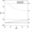 |
Fig. 2 Phase speed diagram of wave modes under photospheric conditions. We have taken cA,i = 2cs,i, cA,e = 0.5cs,i, and cs,e = 1.5cs,i. The Alfvén speeds are not indicated in the graph because no modes with real frequencies appear in that vicinity. The modes with phase speeds between cT,i and cs,i are body modes and the other modes are surface modes. We note that we only plotted two body modes, while there are infinitely many radial overtones. |
To calculate the energy in sausage modes we follow the method by Goossens et al. (2013a; see also the correction for the typographic error in Goossens et al. 2013b). This method is based on the method described in Sect. 9.3 of the book by Walker (2005). The analysis by Goossens et al. (2013a) is valid for MHD waves in a pressureless plasma. In the present paper plasma pressure is taken into account. This introduces additional terms related to the thermal energy. To calculate the energy we use quantities that are averaged over a complete cycle of the wave. The averaged kinetic energy ⟨ KE ⟩, the averaged magnetic energy ⟨ ME ⟩, the averaged thermal energy ⟨ IE ⟩, the averaged total energy ⟨ TE ⟩, the averaged Poynting flux ⟨ S ⟩, the averaged flux of thermal energy ⟨ T ⟩, and the averaged flux of energy ⟨ F ⟩ are given by ![Mathematical equation: \begin{eqnarray} \brac{KE}& =& \frac{\rho_0}{4}\left(\vec{v}\cdot\vec{v^*}\right), \nonumber\\[1.5mm] \brac{ME}&=&\frac{1}{4\mu_0}\left(\vec{B'}\cdot\vec{B'^*}\right), \nonumber\\[1.5mm] \brac{IE}&=&\frac{1}{4\rho_0c_{\mathrm{s}}^2}\left(p' p'^*\right), \nonumber\\[1.5mm] \brac{TE}&=&\brac{KE}+\brac{ME}+\brac{IE}, \nonumber\\[1.5mm] \brac{\vec{S}}&=&\frac{1}{2}\mathrm{Re}\left\{\frac{\vec{E'}\times\vec{B'^*}}{\mu_0}\right\} \!, \nonumber\\[1.5mm] \brac{\vec{T}}&=&\frac{1}{2}\mathrm{Re}\left\{p' \vec{v^*}\right\}\!, \nonumber\\[1.5mm] \brac{\vec{F}}&=&\brac{\vec{S}}+\brac{\vec{T}} \label{eq:energy_gen}, \end{eqnarray}](/articles/aa/full_html/2015/06/aa25468-14/aa25468-14-eq42.png) (4)where μ0 is the magnetic permittivity and an asterix denotes the complex conjugate of a quantity. We note that the expressions describe energy density since the dimension of energy is J/m3. The energy flux is expressed in W/m2.
(4)where μ0 is the magnetic permittivity and an asterix denotes the complex conjugate of a quantity. We note that the expressions describe energy density since the dimension of energy is J/m3. The energy flux is expressed in W/m2.
When considering the energy equations it can seem strange that the energy equations are quadratic in nature for linear wave modes. However, the method described in Walker (2005) uses only first-order reduced MHD equations. The energy equations also contain no linear terms because these integrate to zero over a period/wavelength. On the other hand, it is true that when the observed waves are non-linear in nature, the linear energy equations might no longer be valid. Therefore, we have calculated the largest radial component of the Lagrangian displacement in order to still be a linear MHD wave. It is straightforward to obtain a link between ξr/R and ρ′/ρ0 and this shows that ξr/R can be of the order of a few percent. These small displacements are observable (e.g. Moreels et al. 2015; Grant et al., in prep.), but not all MHD wave mode observations are linear (e.g. Morton et al. 2012a). When applying the linear energy equations to non-linear systems there can be an overestimate of the energy and energy flux owing to non-linear saturation of the system. Using Eqs. (3)we can rewrite Eqs. (4)to find ![Mathematical equation: \begin{eqnarray} \brac{KE} &=& \frac{\rho_0\omega^2}{4}\left(\vec{\xi}\cdot\vec{\xi^*}\right), \nonumber\\[2mm] \brac{ME}&=&\frac{\rho_0k^2c_{\mathrm{A}}^2}{4}(\xi_r \xi_r^*)+\frac{\rho_0c_{\mathrm{A}}^2}{4}\left[\left(\nabla_\perp\cdot\vec{\xi}\right)\left(\nabla_\perp\cdot\vec{\xi^*}\right)\right] \nonumber\\[2mm] &=&\frac{\rho_0k^2c_{\mathrm{A}}^2}{4}(\xi_r \xi_r^*)+\frac{\rho_0c_{\mathrm{A}}^2}{4}\left(\frac{\partial\xi_r}{\partial r}\frac{\partial\xi_r^*}{\partial r}\right) , \nonumber\\[2mm] \brac{IE}&=&\frac{\rho_0c_{\mathrm{s}}^2}{4}\left[\left(\nabla\cdot\vec{\xi}\right)\left(\nabla\cdot\vec{\xi}^*\right)\right], \nonumber\\[2mm] \brac{TE}&=&\brac{KE}+\brac{ME}+\brac{IE}, \nonumber\\[2mm] \brac{\vec{S}}&=&\frac{-1}{2}\mathrm{Re}\left\{\left({\rm i}\rho_0\omega c_{\mathrm{A}}^2 \left(\nabla_\perp\cdot\vec{\xi^*}\right)\xi_r\right)\vec{1_r}+\left(\rho_0 k\omega c_{\mathrm{A}}^2 \xi_r \xi_r^*\right)\vec{1_{\textit{z}}}\right\}, \nonumber\\[2mm] \brac{\vec{T}}&=&\frac{-1}{2}\mathrm{Re}\left\{{\rm i}\omega\rho_0c_{\mathrm{S}}^2\left(\nabla\cdot\vec{\xi}\right)\vec{\xi^*}\right\}, \nonumber\\[2mm] \brac{\vec{E}}&=&\brac{\vec{S}}+\brac{\vec{T}} \label{eq:energy_appl}. \end{eqnarray}](/articles/aa/full_html/2015/06/aa25468-14/aa25468-14-eq48.png) (5)Equations (5)allow us to calculate the energy for any wave mode in a cylindrical plasma structure.
(5)Equations (5)allow us to calculate the energy for any wave mode in a cylindrical plasma structure.
2.2. Energy inside the flux tube for surface modes
We now have three cases (see Fig. 2) in which to calculate the energy and energy flux. First, the energy inside the flux tube for a surface mode. Second, the energy inside the flux tube for a body mode. Third, the energy outside the flux tube. All three calculations are very similar and we only give the details of the calculation for the energy inside the flux tube for a surface mode. The Eulerian total pressure perturbation for a sausage surface mode is given by  (6)where A is a constant amplitude with dimension J/m3, I0(.) indicates the modified Bessel function of the first kind of order zero, and κi is given by
 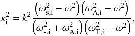 (7)where
  is positive. We have introduced the internal sound frequency ωs,i, the internal Alfvén frequency ωA,i, and the internal tube frequency ωT,i, which are given by ω∗ ,i = kc∗ ,i. We also need expressions for the radial and longitudinal components of the Lagrangian displacement. Using Eqs. (2)and 3 results in
 ![Mathematical equation: \begin{eqnarray} \xi_r(r,z,t)&=&\Xi_r I_1(\kappa_{\mathrm{i}} r) \exp\{{\rm i}(kz-\omega t)\} \label{eq:xi_r},\\[1.5mm] \xi_z(r,z,t)&=&\Xi_z I_0(\kappa_{\mathrm{i}} r) \exp\{{\rm i}(kz-\omega t)\} \label{eq:xi_z}, \end{eqnarray}](/articles/aa/full_html/2015/06/aa25468-14/aa25468-14-eq59.png) where Ξr and Ξz are given by
where Ξr and Ξz are given by 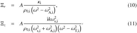 The constants Ξr and Ξz are related to the radial and the longitudinal components of the Lagrangian displacement at the flux tube boundary and have dimension m. Also clear is that Ξr and Ξz are related to each other by the amplitude A; therefore, quantifying the radial component of the Lagrangian displacement results in a measure for the longitudinal component of the Lagrangian displacement and the other way around as well. Later on we use the notation
  and
and  , which are the radial and the longitudinal components of the Lagrangian displacement at the flux tube boundary, respectively, and are given by
 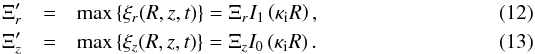 Calculating the magnetic energy also requires the divergence of the Lagrangian displacement, which is given in Eqs. (3)and results in
 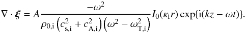 (14)Using Eqs. (6)–(14)we can now calculate the averaged energy and the averaged energy flux inside the flux tube (Eqs. (5)), and we find
 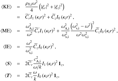 where
where  and
and  are constants and are given by
 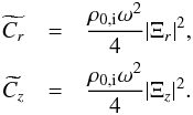 We point out that the constants and have dimension J/m3 as expected. The total energy flux is in the z direction as it should be for trapped wave modes. However, when looking at leaky wave modes there should be energy flux components in the radial direction as well. The total Eulerian pressure perturbation for leaky wave modes is represented by a Hankel function (e.g. Cally 1986; Vasheghani Farahani et al. 2014), i.e. P′(r,z,t) = AH0(κir)exp { i(kz − ωt) }, where H0(κir) = J0(κir) + iY0(κir). When substituting this type of function in Eqs. (5)we find radial components in the energy flux. These radial components are due to the phase shift between the magnetic and the electric field.
At this point the quantities ⟨ KE ⟩, ⟨ ME ⟩, ⟨ IE ⟩, ⟨ S ⟩, and ⟨ T ⟩ depend on the radial position. We now define integrated quantities as 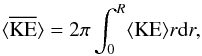 and similarly for
  ,
,  ,
,  , and
, and  . We thus integrate the energy over the tube cross-section, and thus discuss the energy per unit length along the magnetic field. To calculate the total energy we should also integrate over the z-direction from a height zero to a height L, where L is the length of the flux tube (see Van Doorsselaere et al. 2014). Since the wave mode properties do not change with height this results in a simple multiplication with a factor L. Closed analytic expressions for
  , , , , and
  can be found when using Eqs. (9.6.26) and (9.6.28) in Abramowitz & Stegun (1972), i.e. when using
 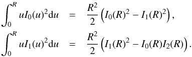 We find that the integrated energy inside a flux tube for a surface mode is given by
 ![Mathematical equation: \begin{eqnarray} \bracs{KE}&=&C_{r}\left(\kappa_{\mathrm{i}} R\right)^2\left(I_1\left(\kappa_{\mathrm{i}}R\right)^2-I_0\left(\kappa_{\mathrm{i}}R\right)I_2\left(\kappa_{\mathrm{i}}R\right)\right)\nonumber\\[1mm] &&\quad +C_{z}(kR)^2\left(I_0\left(\kappa_{\mathrm{i}}R\right)^2-I_1\left(\kappa_{\mathrm{i}}R\right)^2\right),\nonumber\\[1mm] \bracs{ME}&=&\frac{\omega_{\mathrm{A,i}}^2}{\omega^2}C_{r} \left(\kappa_{\mathrm{i}} R\right)^2\left(I_1\left(\kappa_{\mathrm{i}}R\right)^2- I_0\left(\kappa_{\mathrm{i}}R\right)I_2\left(\kappa_{\mathrm{i}}R\right)\right)\nonumber\\[1mm] & &\quad +\frac{\omega_{\mathrm{A,i}}^2}{\omega_{\mathrm{s,i}}^2}\frac{\left(\omega_{\mathrm{s,i}}^2-\omega^2\right)^2}{\omega^2\omega_{\mathrm{s,i}}^2}C_{z}(kR)^2\left(I_0\left(\kappa_{\mathrm{i}}R\right)^2-I_1\left(\kappa_{\mathrm{i}}R\right)^2\right),\nonumber\\[1mm] \bracs{IE}&=&\frac{\omega^2}{\omega_{\mathrm{s,i}}^2}C_{z}(kR)^2\left(I_0 \left(\kappa_{\mathrm{i}}R\right)^2-I_1\left(\kappa_{\mathrm{i}}R\right)^2\right),\nonumber\\[1mm] \bracs{TE}&=&\bracs{KE}+\bracs{ME}+\bracs{IE}, \nonumber\\[1mm] \bracs{\vec{S}}&=&2 \frac{c_{\mathrm{A,i}}^2}{\omega/k} C_{r}\left(\kappa_{\mathrm{i}} R\right)^2\left(I_1(\kappa_{\mathrm{i}}R)^2-I_0\left(\kappa_{\mathrm{i}}R\right)I_2\left(\kappa_{\mathrm{i}}R\right)\right) \vec{1_{\textit{z}}}, \nonumber\\[1mm] \bracs{\vec{T}}&=&2 \frac{\omega}{k} C_{z}(kR)^2\left(I_0\left(\kappa_{\mathrm{i}}R\right)^2-I_1\left(\kappa_{\mathrm{i}}R\right)^2\right) \vec{1_{\textit{z}}}, \nonumber\\[1mm] \bracs{\vec{F}}&=&\bracs{\vec{S}}+\bracs{\vec{T}}, \label{eq:energy} \end{eqnarray}](/articles/aa/full_html/2015/06/aa25468-14/aa25468-14-eq84.png) (15)where Cr and Cz are given by
(15)where Cr and Cz are given by ![Mathematical equation: \begin{eqnarray} C_{r}&=&\pi \frac{\widetilde{C_{r}}}{\kappa_{\mathrm{i}}^2} = \pi\frac{\rho_{0,\mathrm{i}}\omega^2}{4}\frac{|\Xi_r|^2}{\kappa_{\mathrm{i}}^2}=\frac{\pi|A|^2}{4\rho_{0,\mathrm{i}}}\frac{\omega^2}{\left(\omega^2-\omega_{\mathrm{A,i}}^2\right)^2}, \nonumber\\[1mm] C_{z}&=&\pi \frac{\widetilde{C_{z}}}{k^2} = \pi\frac{\rho_{0,\mathrm{i}}\omega^2}{4}\frac{|\Xi_z|^2}{k^2}=\frac{\pi|A|^2}{4\rho_{0,\mathrm{i}}}\frac{\omega^2 \omega_{\mathrm{s,i}}^4}{\left(\omega_{\mathrm{s,i}}^2+\omega_{\mathrm{A,i}}^2\right)^2\left(\omega^2-\omega_{\mathrm{T,i}}^2\right)^2}\cdot\label{eq:constants} \end{eqnarray}](/articles/aa/full_html/2015/06/aa25468-14/aa25468-14-eq87.png) (16)It can easily be checked that the energy is now expressed in J/m and the energy flux is expressed in W. As can be seen from Eqs. (15)the thermal energy and thermal energy flux depend on the plasma motions along the magnetic field, i.e. they are proportional to | Ξz | 2. On the other hand, the Poynting flux depends on the motions perpendicular to the magnetic field, i.e. it is proportional to | Ξr | 2.
(16)It can easily be checked that the energy is now expressed in J/m and the energy flux is expressed in W. As can be seen from Eqs. (15)the thermal energy and thermal energy flux depend on the plasma motions along the magnetic field, i.e. they are proportional to | Ξz | 2. On the other hand, the Poynting flux depends on the motions perpendicular to the magnetic field, i.e. it is proportional to | Ξr | 2.
2.3. Energy inside the flux tube for body modes and external energy
We can do a similar calculation for the energy inside the flux tube for body modes. The only change is the integration of the Bessel functions. For a body mode the pressure perturbation is given by P′(r,z,t) = AJ0(nir)exp { i(kz − ωt) }, where A is a constant amplitude, J0(.) indicates the Bessel function of the first kind of order zero, and  and is positive. As before, closed analytic expressions for the energy and flux of energy can be found when using the following integrals:
 ![Mathematical equation: \begin{eqnarray*} \int_0^R uJ_0(u)^2 {\rm d}u &=& \frac{R^2}{2}\left(J_0(R)^2+J_1(R)^2\right), \\[1.5mm] \int_0^R uJ_1(u)^2 {\rm d}u &=& \frac{R^2}{2}\left(J_1(R)^2-J_0(R)J_2(R)\right). \end{eqnarray*}](/articles/aa/full_html/2015/06/aa25468-14/aa25468-14-eq95.png) These integrals can be checked with Eqs. (9.1.27) and (9.1.28) in Abramowitz & Stegun (1972). The result for the averaged energy and averaged energy flux for body modes is
These integrals can be checked with Eqs. (9.1.27) and (9.1.28) in Abramowitz & Stegun (1972). The result for the averaged energy and averaged energy flux for body modes is ![Mathematical equation: \begin{eqnarray} \bracs{KE}&=&C_{r}(n_{\mathrm{i}} R)^2\left(J_1(n_{\mathrm{i}}R)^2-J_0(n_{\mathrm{i}}R)J_2(n_{\mathrm{i}}R)\right)\nonumber\\[2mm] &&\quad +C_{z}(kR)^2\left(J_0(n_{\mathrm{i}}R)^2+J_1(n_{\mathrm{i}}R)^2\right),\nonumber\\[2mm] \bracs{ME}&=&\frac{\omega_{\mathrm{A,i}}^2}{\omega^2}C_{r}(n_{\mathrm{i}} R)^2\left(J_1(n_{\mathrm{i}}R)^2-J_0(n_{\mathrm{i}}R)J_2(n_{\mathrm{i}}R)\right)\nonumber\\[2mm] &&\quad +\frac{\omega_{\mathrm{A,i}}^2}{\omega_{\mathrm{s,i}}^2}\frac{\left(\omega_{\mathrm{s,i}}^2-\omega^2\right)^2}{\omega^2\omega_{\mathrm{s,i}}^2}C_{z}(kR)^2\left(J_0(n_{\mathrm{i}}R)^2+J_1(n_{\mathrm{i}}R)^2\right),\nonumber\\[2mm] \bracs{IE}&=&\frac{\omega^2}{\omega_{\mathrm{s,i}}^2}C_{z}(kR)^2\left(J_0(n_{\mathrm{i}}R)^2+J_1(n_{\mathrm{i}}R)^2\right),\nonumber\\[2mm] \bracs{TE}&=&\bracs{KE}+\bracs{ME}+\bracs{IE}, \nonumber\\[2mm] \bracs{\vec{S}}&=&2 \frac{c_{\mathrm{A,i}}^2}{\omega/k} C_{r}(n_{\mathrm{i}} R)^2\left(J_1(n_{\mathrm{i}}R)^2-J_0(n_{\mathrm{i}}R)J_2(n_{\mathrm{i}}R)\right) \vec{1_{\textit{z}}}, \nonumber\\[2mm] \bracs{\vec{T}}&=&2 \frac{\omega}{k} C_{z}(kR)^2\left(J_0(n_{\mathrm{i}}R)^2+J_1(n_{\mathrm{i}}R)^2\right) \vec{1_{\textit{z}}}, \nonumber\\[2mm] \bracs{\vec{F}}&=&\bracs{\vec{S}}+\bracs{\vec{T}}, \label{eq:energy_body} \end{eqnarray}](/articles/aa/full_html/2015/06/aa25468-14/aa25468-14-eq96.png) (17)where Cr and Cz are given by Eqs. (16).
(17)where Cr and Cz are given by Eqs. (16).
In the same manner we can calculate the energy outside the flux tube. There are several changes in the derivation. First, the integration of the Bessel function changes, since externally the wave is written by P′(r,z,t) = AK0(κer)exp { i(kz − ωt) }, where A is a constant amplitude, K0(.) indicates the modified Bessel function of the second kind of order zero, and  is the same as but with equilibrium parameters outside the flux tube. Second, the integrated quantities are now defined as
 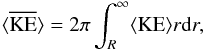 (18)i.e. integrating over the entire domain outside the flux tube. To obtain closed analytic expressions for the energy and flux of energy we use Eqs. (9.6.26) and (9.6.28) in Abramowitz & Stegun (1972), i.e. we use
 ![Mathematical equation: \begin{eqnarray*} \int_R^{\infty} uK_0(u)^2 {\rm d}u &= &\frac{1}{2}\left[u^2K_0(u)^2-u^2K_1(u)^2\right]_R^{\infty}, \\[1.5mm] \int_R^{\infty} uK_1(u)^2 {\rm d}u &= &\frac{1}{2}\left[u^2K_1(u)^2-u^2K_0(u)K_2(u)\right]_R^{\infty}. \end{eqnarray*}](/articles/aa/full_html/2015/06/aa25468-14/aa25468-14-eq101.png) One can easily see that all terms at infinity are zero, e.g. limu → + ∞u2K0(u)2 = 0. The result for the averaged energy and averaged energy flux for the energy outside the flux tube is
One can easily see that all terms at infinity are zero, e.g. limu → + ∞u2K0(u)2 = 0. The result for the averaged energy and averaged energy flux for the energy outside the flux tube is ![Mathematical equation: \begin{eqnarray} \bracs{KE}&=&C_{r}(\kappa_{\mathrm{e}} R)^2\left(K_0(\kappa_{\mathrm{e}}R)K_2(\kappa_{\mathrm{e}}R)-K_1(\kappa_{\mathrm{e}}R)^2\right)\nonumber\\[1.8mm] &&\quad +C_{z}(kR)^2\left(K_1(\kappa_{\mathrm{e}}R)^2-K_0(\kappa_{\mathrm{e}}R)^2\right),\nonumber\\[1.8mm] \bracs{ME}&=&\frac{\omega_{\mathrm{A,e}}^2}{\omega^2}C_{r}(\kappa_{\mathrm{e}} R)^2\left(K_0(\kappa_{\mathrm{e}}R)K_2(\kappa_{\mathrm{e}}R)-K_1(\kappa_{\mathrm{e}}R)^2\right)\nonumber\\[1.8mm] &&\quad +\frac{\omega_{\mathrm{A,e}}^2}{\omega_{\mathrm{s,e}}^2}\frac{\left(\omega_{\mathrm{s,e}}^2-\omega^2\right)^2}{\omega^2\omega_{\mathrm{s,e}}^2}C_{z}(kR)^2\left(K_1(\kappa_{\mathrm{e}}R)^2-K_0(\kappa_{\mathrm{e}}R)^2\right),\nonumber\\[1.8mm] \bracs{IE}&=&\frac{\omega^2}{\omega_{\mathrm{s,e}}^2}C_{z}(kR)^2\left(K_1(\kappa_{\mathrm{e}}R)^2-K_0(\kappa_{\mathrm{e}}R)^2\right),\nonumber\\[1.8mm] \bracs{TE}&=&\bracs{KE}+\bracs{ME}+\bracs{IE}, \nonumber\\[1.8mm] \bracs{\vec{S}}&=&2 \frac{c_{\mathrm{A,e}}^2}{\omega/k} C_{r}(\kappa_{\mathrm{e}} R)^2\left(K_0(\kappa_{\mathrm{e}}R)K_2(\kappa_{\mathrm{e}}R)-K_1(\kappa_{\mathrm{e}}R)^2\right) \vec{1_{\textit{z}}}, \nonumber\\[1.8mm] \bracs{\vec{T}}&=&2 \frac{\omega}{k} C_{z}(kR)^2\left(K_1(\kappa_{\mathrm{e}}R)^2-K_0(\kappa_{\mathrm{e}}R)^2\right) \vec{1_{\textit{z}}}, \nonumber\\[1.8mm] \bracs{\vec{F}}&=&\bracs{\vec{S}}+\bracs{\vec{T}}, \label{eq:energy_ext} \end{eqnarray}](/articles/aa/full_html/2015/06/aa25468-14/aa25468-14-eq103.png) (19)where Cr and Cz are given by Eqs. (16)but with all equilibrium parameters taken outside the flux tube.
(19)where Cr and Cz are given by Eqs. (16)but with all equilibrium parameters taken outside the flux tube.
Equations (15)–(19)allow us to calculate the energy in sausage mode in a general cylindrical plasma structure, i.e. we have not restricted ourselves to coronal flux tubes. As input we need the radius of the flux tube, the sound and Alfvén speeds, the plasma density, the period and phase speed of the wave, and the radial or longitudinal component of the Lagrangian displacement at the flux tube boundary. We stress that only the radial or the longitudinal component of the Lagrangian displacement is needed since both are linked through the amplitude A as mentioned earlier. All of these are available with modern ground- or space-based observations combined with empirical solar atmospheric models (e.g. recent work by Morton et al. 2011; Dorotovič et al. 2014; Moreels et al. 2015). Our equations are generally valid and can be used to calculate the energy and energy flux in the observed axisymmetric waves.
The group speed vg is defined as  (20)where
  is the sum of both the internal and external flux of energy and
  also includes both internal and external energy. In this way the group speed expresses the propagation speed of energy.
3. Limiting cases
In this section we study some cases of physical interest, i.e. sausage modes in thin flux tubes. Figure 3 shows the dispersion diagram under coronal conditions. We have two types of wave modes, i.e. fast and slow sausage body modes. We only plotted one slow body mode and five fast body modes, while there are actually many radial overtones. We begin by studying slow sausage modes (Sect. 3.1) in thin (coronal) flux tubes and afterwards we look at fast sausage modes (Sect. 3.2) in coronal flux tubes at the cut-off wavenumber. The extra assumptions that are made in the section are usually valid in the solar corona, but care needs to be taken with the thin tube limit. Aschwanden et al. (2004) explained that coronal loops may oscillate with higher harmonics, which would result in the thin tube limit not being applicable, and that the use of the full energy equations from Sect. 2.2 should be applied. We stress that this section of limiting cases uses extra assumptions that are not necessarily valid in different layers of the solar atmosphere. Therefore, care needs to be taken when utilizing the results from limiting cases and in some cases it may be that the full set of energy Eqs. (15)provide a more accurate result.
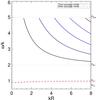 |
Fig. 3 Phase speed diagram of wave modes under coronal conditions. We have taken cA,i = 2cs,i, cA,e = 5cs,i, and cs,e = 0.5cs,i. All modes are body modes. For the slow modes we only plotted one mode, for the fast modes we plotted five modes, while for both there are an infinite number of radial overtones. |
3.1. Slow waves
In this section we look at the limiting case of slow waves in thin flux tubes. In the literature there has been extensive study on slow magnetoaccoustic waves (see De Moortel 2009, for an overview). From these studies we know that the energy of the wave should propagate along the magnetic field at the local tube speed. We begin by giving the dispersion relation for slow sausage body modes (see Edwin & Roberts 1983), 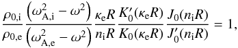 (21)where the dash denotes the derivative of a Bessel function (e.g.
 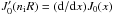 evaluated at x = niR) and where
  is given by Eq. (7). We also study slow sausage surface modes, which do not occur under coronal conditions but do occur under photospheric conditions (see Fig. 2). The dispersion relation is slightly different, i.e.
 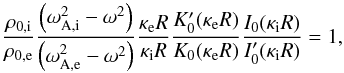 (22)but the calculations will not be very different. We study slow waves in thin flux tubes, meaning that kR goes to zero. When looking at the phase diagram (Fig. 2 or Fig. 3) we notice that the phase speed of slow waves approaches the internal tube speed as kR becomes smaller. After studying the dispersion relation (Eq. (21)) we found that as kR → 0 the frequency of body modes is given by ω = ωT,i + (kR)2ln(kR)ω1. For surface modes the + sign is replaced with a − sign. Expanding the Bessel functions that appear in the dispersion relation (Eq. (21)) results in a non-zero ω1 given by
 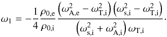 (23)We want to make several remarks on this dispersive correction term ω1(kR)2ln(kR). First, the expression for ω1 is not needed in the long wavelength limit (i.e. kR = 0). Second, the expression for ω1 has the correct dimension, i.e. it is a frequency. Third, under coronal conditions the sign is negative as we would expect since slow body waves have higher phase speed than the internal tube speed. Fourth, this formula is only valid for the fundamental body mode, not for radial overtones because of the expansions of the Bessel functions we have used, i.e. we assumed that niR ≪ 1, while for radial overtones this is not the case. Fifth, the formula for ω1 is not valid under photospheric conditions. Figure 3 in Moreels & Van Doorsselaere (2013) shows that the fundamental slow sausage body mode under photospheric conditions has one node inside the flux tube in the eigenfunctions, meaning that niR is not small and our expansions of the Bessel functions are not valid. Because of these restrictions, this formula is only valid for the fundamental body mode under coronal conditions.
In expanding the Bessel functions we used 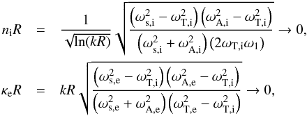 where we retained terms up to (kR)2ln(kR). The constants Cr and Cz are written in several forms; one of which uses unknown amplitude A. We can find the amplitude A by looking at the Lagrangian displacement and the pressure perturbation (Eqs. (6), (8), and (9)). We know that all these must remain finite, also at the flux tube boundary. We have defined to indicate the maximum longitudinal component of the Lagrangian displacement at the flux tube boundary. This is related to the variable Ξz by
  , meaning that for thin flux tubes we have
  . Assuming that is finite, combined with the continuity of the pressure perturbation allows us to find an expression for both the internal amplitude Ai and the external amplitude Ae. These are given by
 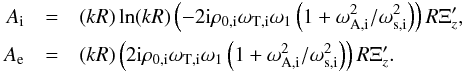 We note that these are just Eqs. (10)and (11)applied to body modes in thin flux tubes. When using these amplitudes we find that both the pressure perturbation and the radial component of the Lagrangian displacement inside the flux tube go to zero as (kR)ln(kR) goes to zero. The longitudinal component of the Lagrangian displacement inside the flux tube is approximately constant and is non-zero. The pressure perturbation, the radial component of the Lagrangian displacement, and the longitudinal component of the Lagrangian displacement outside the flux tube go to zero as kR goes to zero.
We now calculate the energy for slow sausage modes in the long wavelength limit (i.e. kR = 0) and we find ![Mathematical equation: \begin{eqnarray} \bracs{KE}&=&\frac{\rho_{0\mathrm{,i}}}{4}\omega_{\mathrm{T,i}}^2 \pi R^2 \Xi_z'^2, \nonumber\\[1mm] \bracs{ME}&=&\frac{\rho_{0\mathrm{,i}}}{4}\omega_{\mathrm{T,i}}^2 \pi R^2 \Xi_z'^2\frac{\omega_{\mathrm{T,i}}^2}{\omega_{\mathrm{A,i}}^2}, \nonumber\\[1mm] \bracs{IE}&=&\frac{\rho_{0\mathrm{,i}}}{4}\omega_{\mathrm{T,i}}^2 \pi R^2 \Xi_z'^2\frac{\omega_{\mathrm{T,i}}^2}{\omega_{\mathrm{s,i}}^2},\nonumber\\[1mm] \bracs{TE}&=&\frac{\rho_{0\mathrm{,i}}}{2}\omega_{\mathrm{T,i}}^2 \pi R^2 \Xi_z'^2,\nonumber\\[1mm] \bracs{\vec{S}}&=&\vec{0}, \nonumber\\[1mm] \bracs{\vec{T}}&=&\frac{\rho_{0\mathrm{,i}}}{2}\omega_{\mathrm{T,i}}^2 \pi R^2 \Xi_z'^2 c_{\mathrm{T,i}} \vec{1_{\textit{z}}}, \nonumber\\[1mm] \vec{v}_\mathrm{g}&=&c_{\mathrm{T,i}}\vec{1_{\textit{z}}} \label{eq:slow_mode}. \end{eqnarray}](/articles/aa/full_html/2015/06/aa25468-14/aa25468-14-eq134.png) (24)As before, the energy is expressed in J/m and the energy flux is expressed in W. The energy is contained entirely inside the flux tube, i.e. the energy outside the flux tube is zero. This was to be expected since we already found that the perturbations outside the flux tube go to zero as kR goes to zero. We also retrieve the expected equipartition of energy between the potential energy (i.e. the sum of both magnetic and thermal energy) and the kinetic energy. The group speed is exactly equal to the tube speed and is directed along the magnetic field. We remark that these formulas are applicable in different regions of the solar atmosphere, both in the corona and in the photosphere. Previously, we stressed that the dispersive correction ω1(kR)2ln(kR) was only valid for fundamental body modes under coronal conditions. However, as mentioned before, in deriving Eqs. (24)we did not need Eq. (23), which describes ω1. The constant ω1 cancelled out in the long wavelength limit, showing that Eqs. (24)are also valid under photospheric conditions. In Appendix A we list the complete expressions for slow wave modes in thin flux tubes, i.e. with a small but non-zero value of kR. The expressions in Appendix A are valid for the fundamental slow body mode under coronal conditions and for the surface mode under photospheric conditions.
(24)As before, the energy is expressed in J/m and the energy flux is expressed in W. The energy is contained entirely inside the flux tube, i.e. the energy outside the flux tube is zero. This was to be expected since we already found that the perturbations outside the flux tube go to zero as kR goes to zero. We also retrieve the expected equipartition of energy between the potential energy (i.e. the sum of both magnetic and thermal energy) and the kinetic energy. The group speed is exactly equal to the tube speed and is directed along the magnetic field. We remark that these formulas are applicable in different regions of the solar atmosphere, both in the corona and in the photosphere. Previously, we stressed that the dispersive correction ω1(kR)2ln(kR) was only valid for fundamental body modes under coronal conditions. However, as mentioned before, in deriving Eqs. (24)we did not need Eq. (23), which describes ω1. The constant ω1 cancelled out in the long wavelength limit, showing that Eqs. (24)are also valid under photospheric conditions. In Appendix A we list the complete expressions for slow wave modes in thin flux tubes, i.e. with a small but non-zero value of kR. The expressions in Appendix A are valid for the fundamental slow body mode under coronal conditions and for the surface mode under photospheric conditions.
We averaged the flux of energy across a surface perpendicular to the magnetic field resulting in  . The surface over which we averaged is a circular disk with radius df. The idea behind this averaging over an area is linked to the paper by Van Doorsselaere et al. (2014). In that paper MHD theory is used to write an expression for energy flux in multistrand coronal loops in terms of density filling factors. As explained in Van Doorsselaere et al. (2014) the radius of a flux tube strand R can be linked with the influence radius of that flux tube strand df using the density filling factor f, i.e.
  (25)The averaging results in
 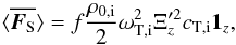 (26)where the averaged flux is now dependent on the density filling factor f. We note that the dimension of is W/m2.
For slow waves in the footpoints of thin coronal flux tubes we can make the extra assumption that the plasma beta is low (i.e. β ≪ 1). We find that  , where γ is the ratio of specific heats. For the energy we find
 ![Mathematical equation: \begin{eqnarray} \bracs{KE}&=&\frac{\rho_{0\mathrm{,i}}}{4}\omega_{\mathrm{T,i}}^2 \pi R^2 \Xi_z'^2, \nonumber\\[1mm] \bracs{ME}&=&\frac{\rho_{0\mathrm{,i}}}{4}\omega_{\mathrm{T,i}}^2 \pi R^2 \Xi_z'^2 \frac{\gamma}{2}\beta, \nonumber\\[1mm] \bracs{IE}&=&\frac{\rho_{0\mathrm{,i}}}{4}\omega_{\mathrm{T,i}}^2 \pi R^2 \Xi_z'^2 \left(1-\frac{\gamma}{2}\beta\right), \nonumber\\[1mm] \bracs{\vec{S}}&=&\vec{0}, \nonumber\\[1mm] \bracs{\vec{T}}&=&2 \frac{\rho_{0\mathrm{,i}}}{4}\omega_{\mathrm{T,i}}^2 \pi R^2 \Xi_z'^2 c_{\mathrm{T,i}} \vec{1_{\textit{z}}}, \nonumber\\[1mm] \vec{v}_\mathrm{g}&=&c_{\mathrm{s,i}}\left(1+\frac{\gamma}{2}\beta\right) \vec{1_{\textit{z}}} \label{eq:slow_mode_low_beta}. \end{eqnarray}](/articles/aa/full_html/2015/06/aa25468-14/aa25468-14-eq143.png) (27)When the plasma beta is equal to zero we still have equipartition between kinetic and potential energy, but the potential energy is only thermal energy with no contribution of magnetic energy. We also find that energy is transported along the field lines at the internal tube speed, which is equal to the internal sound speed. Therefore, these waves are very like sound waves in a non-magnetised atmosphere, except these waves travel along the magnetic field.
(27)When the plasma beta is equal to zero we still have equipartition between kinetic and potential energy, but the potential energy is only thermal energy with no contribution of magnetic energy. We also find that energy is transported along the field lines at the internal tube speed, which is equal to the internal sound speed. Therefore, these waves are very like sound waves in a non-magnetised atmosphere, except these waves travel along the magnetic field.
3.2. Fast waves
In this section we study fast sausage modes under coronal conditions. The fast sausage modes can be seen in the coronal dispersion diagram (Fig. 3) and their dispersion curves are shown with full lines. In particular we study the fundamental fast sausage mode, but radial overtones are also discussed. We immediately put plasma beta equal to zero since this eliminates only the slow modes from the dispersion diagram, not the fast modes. We split the discussion into two parts, one dealing with the energy inside the flux tube and the other outside the flux tube.
3.2.1. Energy inside the flux tube
The dispersion relation for body modes has already been given in Eq. (21). Following the same calculation as Vasheghani Farahani et al. (2014) we find that the solution of the dispersion relation at the cut-off wavenumber kc is given by ω = ωA,e, niR = j0,1, and  where j0,1 is the first zero of the Bessel function J0(niR). This is the solution for the fundamental sausage mode; for the lth radial overtone we need to replace j0,1 with j0,l, where j0,l is the lth zero of the Bessel function J0(niR).
Unlike the study of slow sausage waves, here we do not need a better approximation of the phase speed around the cut-off wavenumber since no indeterminate forms occur in the energy calculations. We know that  We can now expand the Bessel functions that occur in the energy equations (Eqs. (17)). As was the case for slow modes, here too we need an expression for the unknown amplitude A that appears in the constants Cr and Cz. Again, we determine the amplitude A from Eqs. (10)and (11)applied to body modes. Since we are working in the cold plasma approximation we already know that ξz = 0 everywhere, therefore Eq. (11)cannot be used. As before, we define as the maximum value of the radial component of the Lagrangian displacement at the flux tube boundary, which is linked to Ξr by
  . We know that ξr and P′ must be finite everywhere and non-zero at some point inside the flux tube, otherwise there would be no wave energy inside the flux tube. This happened in the previous limiting case (see Sect. 3.1), where in the long wavelength limit the external wave perturbations were exactly zero and therefore we found no external energy. A possible solution is
 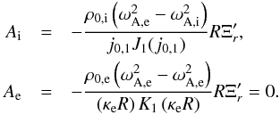 After some straightforward calculations we find that the energy inside the flux tube for fast sausage modes at the cut-off wavenumber in the zero plasma beta approximation is given by
 ![Mathematical equation: \begin{eqnarray} \bracs{KE}_{\mathrm{i}}&=&\frac{\rho_{0\mathrm{,i}}}{4}\omega_{\mathrm{A,e}}^2 \pi R^2 \Xi_r'^2, \nonumber\\[1mm] \bracs{ME}_{\mathrm{i}}&=&\frac{\rho_{0\mathrm{,i}}}{4}\omega_{\mathrm{A,i}}^2 \pi R^2 \Xi_r'^2, \nonumber\\[1mm] \bracs{IE}_{\mathrm{i}}&=&0, \nonumber\\[1mm] \bracs{\vec{S}}_{\mathrm{i}}&=&2\frac{\rho_{0\mathrm{,i}}}{4}\omega_{\mathrm{A,i}}^2 c_{\mathrm{A,e}}\pi R^2 \Xi_r'^2 \vec{1_{\textit{z}}}, \nonumber\\[1mm] \bracs{\vec{T}}_{\mathrm{i}}&=&\vec{0} \label{eq:fast_mode_internal}. \end{eqnarray}](/articles/aa/full_html/2015/06/aa25468-14/aa25468-14-eq156.png) (28)Because we are working in the cold plasma approximation we expect no thermal energy and this is confirmed here. We note that there is no equipartition of energy between magnetic and kinetic energy. This is not a problem since we have not included the external energy at the moment. We have not mentioned the group speed since we have not yet calculated the external energy.
(28)Because we are working in the cold plasma approximation we expect no thermal energy and this is confirmed here. We note that there is no equipartition of energy between magnetic and kinetic energy. This is not a problem since we have not included the external energy at the moment. We have not mentioned the group speed since we have not yet calculated the external energy.
3.2.2. Energy outside the flux tube
We now calculate the external energy for fast sausage modes at the cut-off wavenumber. From Sect. 3.2.1 we already know the complete solution to the dispersion relation and the amplitude Ae. Therefore, we can just use Eqs. (19). We know that the kinetic energy is given by ![Mathematical equation: \begin{eqnarray*} \bracs{KE}_{\mathrm{e}} &=& C_{r}\left(\kappa_{\mathrm{e}} R\right)^2\left(K_0\left(\kappa_{\mathrm{e}}R\right)K_2\left(\kappa_{\mathrm{e}}R\right)-K_1\left(\kappa_{\mathrm{e}}R\right)^2\right)\nonumber\\[1.5mm] & &\quad +C_{z}(kR)^2\left(K_1\left(\kappa_{\mathrm{e}}R\right)^2-K_0\left(\kappa_{\mathrm{e}}R\right)^2\right) \\[1.5mm] &= &\frac{\rho_{0\mathrm{,e}}}{4}\omega_{\mathrm{A,e}}^2 \pi R^2 \Xi_r'^2 \left(-\ln\left(\kappa_{\mathrm{e}}R\right)-1\right). \end{eqnarray*}](/articles/aa/full_html/2015/06/aa25468-14/aa25468-14-eq157.png) In the calculation we have used the small argument expansions for the Bessel functions since κeR = 0. The external kinetic energy resembles the internal kinetic energy, except that the density is taken outside and there is the added (− ln(κeR) − 1) term. It is this last term that is problematic: we know that κeR = 0, and so this term becomes infinitely large.
In the calculation we have used the small argument expansions for the Bessel functions since κeR = 0. The external kinetic energy resembles the internal kinetic energy, except that the density is taken outside and there is the added (− ln(κeR) − 1) term. It is this last term that is problematic: we know that κeR = 0, and so this term becomes infinitely large.
To expand on this case of infinite energy, we first looked at trapped wave modes very close to the cut-off wavenumber numerically, i.e. we numerically integrated Eq. (18)for trapped wave modes. We are dealing with trapped wave modes, therefore we would expect a finite, but possibly large, external energy. We indeed found that for all trapped wave modes the energy is finite, but for kR → kcR the external energy becomes much larger than the energy inside the flux tube. This confirms the mathematical result that at the cut-off wavenumber the external kinetic energy becomes infinite.
An infinitely large kinetic energy is not physically acceptable. The reason that the energy is infinite is quite simple from a mathematical point of view. Sausage waves at the cut-off wavenumber have been represented by Bessel functions. Of course, at the cut-off wavenumber the wave mode becomes leaky and it should be represented by Hankel functions (e.g. Cally 1986; Vasheghani Farahani et al. 2014). Going back to Eq. (18)and substituting ⟨ KE ⟩ by the correct expression with Hankel functions leads to the integral 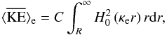 where C is a non-zero constant. The Hankel function squared can be written as
 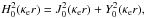 where J0(.) and Y0(.) are Bessel functions of the first and second kind of order zero. This function is not square-integrable, i.e. the function is non-zero at infinity and therefore the integral results in an infinite kinetic energy.
Naturally, there is also a physical reason why the kinetic energy is infinite. Assume that at a certain time t a flux tube in equilibrium is suddenly perturbed such that the excited wave mode is a fast sausage wave at the cut-off wavenumber. Because the wave mode is leaky, the energy will be transported outward from the flux tube at a certain speed V. When we observe this wave mode at time t + Δt and we want to calculate the energy, we need both the energy inside and outside the flux tube. For the energy inside the flux tube we have derived formulas in Sect. 3.2.1. To calculate the external energy we need to realise that the wave energy has only propagated to a distance d = VΔt, because the energy propagates at a velocity V. Therefore the integral we need to compute is not Eq. (18), but we should compute 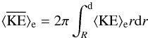 (29)since the energy is zero when going further from the flux tube than a distance d. This formula would give us a finite kinetic energy as we would expect. The shortcoming in the modelling of the wave modes is assuming that these waves exist over the entire infinite domain, while in reality they only exist up to a certain distance d outside the flux tube. We can summarise this particular wave mode as a case where no normal mode solution is found that is physically acceptable, but there is actually a wave mode solution to the initial value problem (Roberts & Boardman 1962).
The physical distance d is almost impossible to quantify directly since the transport of energy is difficult to identify, even using the highest-resolution solar observations. However, there are ways to infer this distance d. We turn to the paper by Van Doorsselaere et al. (2014) and use the influence radius of a flux tube strand  to quantify the distance d. Using this influence radius df in combination with Eq. (29)should result in finite values for the energy of the wave mode. The general calculation, when not using a specific wave mode and when integrating to a distance df, results in equations similar to Eqs. (19)with some adaptations, e.g.
 ![Mathematical equation: \begin{eqnarray} \bracs{KE}_{\mathrm{e}}&=&C_{r} \left(\kappa_{\mathrm{e}} R\right)^2\left[\frac{K_1\left(\kappa_{\mathrm{e}}R/\!\!\sqrt{f}\right)^2- K_0\left(\kappa_{\mathrm{e}}R/\!\!\sqrt{f}\right)K_2\left(\kappa_{\mathrm{e}}R/\!\!\sqrt{f}\right)}{f}\right] \nonumber\\[1.5mm] & &\quad +C_{r}\left(\kappa_{\mathrm{e}} R\right)^2\left[K_0\left(\kappa_{\mathrm{e}}R\right)K_2\left(\kappa_{\mathrm{e}}R\right)-K_1\left(\kappa_{\mathrm{e}}R\right)^2\right] \nonumber\\[1.5mm] & &\quad +C_{z}(kR)^2\left[\frac{K_0\left(\kappa_{\mathrm{e}}R/\!\!\sqrt{f}\right)^2-K_1\left(\kappa_{\mathrm{e}}R/\!\!\sqrt{f}\right)^2}{f}\right] \nonumber\\[1.5mm] &&\quad +C_{z}(kR)^2\left[K_1\left(\kappa_{\mathrm{e}}R\right)^2-K_0\left(\kappa_{\mathrm{e}}R\right)^2\right], \label{eq:KE_external} \end{eqnarray}](/articles/aa/full_html/2015/06/aa25468-14/aa25468-14-eq172.png) (30)where Cr and Cz are given by Eq. (16)taken with values outside the flux tube. We have similar equations for the magnetic energy, the thermal energy, the total energy, the Poynting flux, the flux of thermal energy, and the flux of energy.
(30)where Cr and Cz are given by Eq. (16)taken with values outside the flux tube. We have similar equations for the magnetic energy, the thermal energy, the total energy, the Poynting flux, the flux of thermal energy, and the flux of energy.
We can now proceed as in the case of the energy inside the flux tube for fast waves. We already know the complete solution to the dispersion relation and the amplitude Ae (see Sect. 3.2.1). Therefore we can expand the Bessel functions for small arguments and using Eq. (30)we find that ![Mathematical equation: \begin{eqnarray} \bracs{KE}_{\mathrm{e}}&=&\frac{\rho_{0\mathrm{,e}}}{4}\omega_{\mathrm{A,e}}^2 \pi R^2 \Xi_r'^2 \ln(1/f), \nonumber\\[1.5mm] \bracs{ME}_{\mathrm{e}}&=&\frac{\rho_{0\mathrm{,e}}}{4}\omega_{\mathrm{A,i}}^2 \pi R^2 \Xi_r'^2 \ln(1/f), \nonumber\\[1.5mm] \bracs{IE}_{\mathrm{e}}&=&0, \nonumber\\[1.5mm] \bracs{\vec{S}}_{\mathrm{e}}&=&2\frac{\rho_{0\mathrm{,e}}}{4}c_{\mathrm{A,e}}\omega_{\mathrm{A,e}}^2\pi R^2 \Xi_r'^2 \ln(1/f) \vec{1_{\textit{z}}}, \nonumber\\[1.5mm] \bracs{\vec{T}}_{\mathrm{e}}&=&\vec{0} \label{eq:fast_mode_external}. \end{eqnarray}](/articles/aa/full_html/2015/06/aa25468-14/aa25468-14-eq173.png) (31)These expressions are very similar when compared to the energy equations inside the flux tube (Eqs. (28)), the densities are taken outside the flux tube and there is the extra logarithmic factor. We first check what this logarithmic term implies. We know that the filling factor f is a value between zero and one, meaning that the energy is indeed positive. When the filling factor is one, we find that the energy is zero, which is to be expected. When the filling factor is one, we have df = R and the integral is then calculated on a zero interval. When the filling factor is zero, we find that the energy is infinite. This is also as it should be since for a filling factor of zero we have a single isolated flux tube with df = ∞ and we arrive at the same problem as we had at the start of this section.
(31)These expressions are very similar when compared to the energy equations inside the flux tube (Eqs. (28)), the densities are taken outside the flux tube and there is the extra logarithmic factor. We first check what this logarithmic term implies. We know that the filling factor f is a value between zero and one, meaning that the energy is indeed positive. When the filling factor is one, we find that the energy is zero, which is to be expected. When the filling factor is one, we have df = R and the integral is then calculated on a zero interval. When the filling factor is zero, we find that the energy is infinite. This is also as it should be since for a filling factor of zero we have a single isolated flux tube with df = ∞ and we arrive at the same problem as we had at the start of this section.
3.2.3. Total energy
Finally we now consider the energy for fast sausage waves both inside and outside the flux tube. We easily find that the energy and flux of energy are given by ![Mathematical equation: \begin{eqnarray} \bracs{KE}&=&\frac{\rho_{0\mathrm{,i}}+\rho_{0\mathrm{,e}}\ln(1/f)}{4}\omega_{\mathrm{A,e}}^2 \pi R^2 \Xi_r'^2, \nonumber\\[2mm] \bracs{ME}&=&\frac{\rho_{0\mathrm{,i}}+\rho_{0\mathrm{,e}}\ln(1/f)}{4}\omega_{\mathrm{A,i}}^2 \pi R^2 \Xi_r'^2, \nonumber\\[2mm] \bracs{IE}&=&0, \nonumber\\[2mm] \bracs{TE}&=&\frac{\rho_{0\mathrm{,i}}+\rho_{0\mathrm{,e}}\ln(1/f)}{4}\left(\omega_{\mathrm{A,i}}^2+\omega_{\mathrm{A,e}}^2\right)\pi R^2 \Xi_r'^2, \nonumber\\[2mm] \bracs{\vec{S}}&=&\frac{\rho_{0\mathrm{,i}}\omega_{\mathrm{A,i}}^2+\rho_{0\mathrm{,e}}\omega_{\mathrm{A,e}}^2\ln(1/f)}{2}c_{\mathrm{A,e}} \pi R^2 \Xi_r'^2 \vec{1_{\textit{z}}}, \nonumber\\[2mm] \bracs{\vec{T}}&=&\vec{0}, \nonumber\\[2mm] \bracs{\vec{F}}&=&\frac{\rho_{0\mathrm{,i}}\omega_{\mathrm{A,i}}^2+\rho_{0\mathrm{,e}}\omega_{\mathrm{A,e}}^2\ln(1/f)}{2}c_{\mathrm{A,e}} \pi R^2 \Xi_r'^2 \vec{1_{\textit{z}}}. \label{eq:energy_fast} \end{eqnarray}](/articles/aa/full_html/2015/06/aa25468-14/aa25468-14-eq176.png) (32)We note that there is no equipartition of energy between kinetic and magnetic energy. This should not come as a surprise since we have calculated the external energy only to the point df and equipartition should only exist over the entire space. As before, we also calculated the flux of energy averaged over a surface perpendicular to the flux tube , which is given by
(32)We note that there is no equipartition of energy between kinetic and magnetic energy. This should not come as a surprise since we have calculated the external energy only to the point df and equipartition should only exist over the entire space. As before, we also calculated the flux of energy averaged over a surface perpendicular to the flux tube , which is given by ![Mathematical equation: \begin{eqnarray} \bracs{\vec{F_{\textrm{S}}}}&=&f\frac{\rho_{0\mathrm{,i}}\omega_{\mathrm{A,i}}^2+\rho_{0\mathrm{,e}}\omega_{\mathrm{A,e}}^2\ln(1/f)}{2}c_{\mathrm{A,e}} \Xi_r'^2 \vec{1_{\textit{z}}}, \nonumber\\[2mm] \vec{v}_\mathrm{g}&=&2\frac{\rho_{0\mathrm{,i}}\omega_{\mathrm{A,i}}^2+\rho_{0\mathrm{,e}}\omega_{\mathrm{A,e}}^2\ln(1/f)}{\rho_{0\mathrm{,i}}+\rho_{0\mathrm{,e}}\ln(1/f)}\frac{c_{\mathrm{A,e}}}{\omega_{\mathrm{A,i}}^2+\omega_{\mathrm{A,e}}^2}\vec{1_{\textit{z}}}, \nonumber\\[2mm] &=& 2\frac{1+\ln(1/f)}{1+\ln(1/f)+\zeta+\ln(1/f)/\zeta}c_{\mathrm{A,e}}\vec{1_{\textit{z}}}, \end{eqnarray}](/articles/aa/full_html/2015/06/aa25468-14/aa25468-14-eq177.png) (33)where ζ = ρ0,i/ρ0,e is the density contrast as introduced in Van Doorsselaere et al. (2004a). We note that the flux of energy averaged over a disk with radius df is a finite value for any value of the filling factor f. The group speed depends on the density filling factor f, the density contrast ζ, and the phase speed of the wave cA,e.
(33)where ζ = ρ0,i/ρ0,e is the density contrast as introduced in Van Doorsselaere et al. (2004a). We note that the flux of energy averaged over a disk with radius df is a finite value for any value of the filling factor f. The group speed depends on the density filling factor f, the density contrast ζ, and the phase speed of the wave cA,e.
We consider the result from Morton et al. (2012a), where they observed both sausage and kink modes in the chromosphere and found that the energy of compressive (sausage) waves was larger than the energy in transverse waves. We now have formulas for the energy of fast sausage waves and in Goossens et al. (2013a) or Van Doorsselaere et al. (2014) we can find formulas for the energy in fast kink waves. We assume some realistic values for the filling factor and the density contrast, i.e. f = 0.1 and ζ = 5. We calculate the total energy for both wave modes, i.e. ![Mathematical equation: \begin{eqnarray*} \bracs{TE}_\mathrm{sausage}&=&0.37 \rho_{0\mathrm{,i}} \left(\omega_{\mathrm{A,i}}^2+\omega_{\mathrm{A,e}}^2\right)\Xi_{\mathrm{s}}^2, \\[2mm] \bracs{TE}_\mathrm{kink}&=&0.6 \rho_{0\mathrm{,i}} \omega_{\mathrm{K}}^2 \Xi_{\mathrm{k}}^2, \end{eqnarray*}](/articles/aa/full_html/2015/06/aa25468-14/aa25468-14-eq183.png) where we have normalised the energy with the unit of volume over which the energy was calculated and where
where we have normalised the energy with the unit of volume over which the energy was calculated and where  is the kink frequency. When taking the ratio we find
 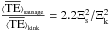 . Hence, the ratio of energy in sausage waves and in kink waves depends on the amplitude of the radial component of the Lagrangian displacement. If these are of the same order we find that
  . This is of the same magnitude as the observations by Morton et al. (2012a) where the authors found a ratio of 2.7 with some uncertainty. Our theory with a realistic filling factor and density ratio thus agrees with the energy ratio found in specific observations between kink and sausage modes.
4. Conclusions
In this paper we have derived formulas to calculate the wave energy in sausage modes. We did this by modelling the flux tube as a straight cylinder with constant radius and constant plasma parameters both inside and outside the flux tube. The formulas can thus be applied to different regions in the solar atmosphere because we did not use the thin tube or low plasma beta approximations. We did, however, neglect density stratification and/or flux tube expansion effects in our equilibrium model, meaning that some care needs to be taken when applying the energy formulas (Eqs. (15), (17), and (19)) to photospheric observations. On the other hand, these effects are less important under coronal conditions, meaning that the limiting cases (see Sect. 3) can be applied readily to coronal or chromospheric observations.
In Sect. 2 we have calculated the energy in wave modes using the complete equilibrium model, i.e. no additional assumptions were made. The resulting equations (Eqs. (15), (17), and (19)) can be applied to both surface and body modes and the energy both inside and outside the flux tube can be calculated. As input for the calculations one needs the sound and Alfvén speeds, the phase speed of the wave, the plasma density, the radius of the flux tube, and the amplitude A that occurs in the mathematical description of the wave. The amplitude A can be linked with either the radial or longitudinal component of the Lagrangian displacement at the flux tube boundary (see Eqs. (16)). All these parameters are available from observations and/or empirical models of the solar atmosphere. The phase speed of the wave is the hardest parameter to determine for observations in the lower solar atmosphere, since observations are only taken at one or a few heights in the magnetic structure. A method for determining the phase speed of waves using only intensity images at one height in the solar atmosphere has been described in Moreels et al. (2015). The key to determining the phase speed is to be able to identify the fractional changes in intensity and area, for which a high resolution is needed. Thus, as we move into the era of the Daniel K. Inouye Solar Telescope (DKIST, formerly known as the Advanced Technology Solar Telescope (ATST), Elmore et al. 2014) and the European Solar Telescope (EST, Collados et al. 2010), this paper combined with Moreels et al. (2015) will provide a way to analyse sausage modes in the lower solar atmosphere as the methods of observation become more advanced. It could also be said that the results of this work will become more accurate over time as the resolution of the data increases, therefore this work will become even more useful in the future.
In Sect. 3 and in Appendix A we have applied the general energy formulas to the case of sausage modes in thin flux tubes (in coronal/chromospheric flux tubes). We have formulas to calculate the energy for slow sausage modes in the long wavelength limit for both general plasma beta (Eqs. (24)) and low plasma beta values (Eqs. (27)). The slow sausage wave is dominated by the longitudinal component of the Lagrangian displacement and therefore the energy is expressed in terms of this displacement. In the long wavelength limit we find the equipartition between kinetic and potential energy. In the cold plasma approximation (i.e. the plasma beta is zero) the potential energy consists only of thermal energy and the magnetic energy is exactly zero. The group speed is equal to the internal tube speed, as expected. In Appendix A we list the energy equations for both the fundamental slow sausage body mode under coronal conditions and the sausage surface mode under photospheric conditions in thin flux tubes (i.e. kR is small but non-zero). In this section we also found the dispersive first-order correction to the phase speed in the thin tube limit for both the fundamental slow sausage body mode under coronal conditions and the sausage surface mode under photospheric conditions. From an observational point of view the most important quantity is the averaged flux of energy through a surface perpendicular to the flux tube , which is given by 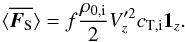 (34)The flux is expressed in W/m2 and can easily be calculated. In the above formula f is the filling factor which is available in most observations. The equilibrium density inside the flux tube ρ0,i can be found from empirical models of the solar atmosphere. We also have
  , which is the longitudinal component of the velocity perturbation at the flux tube boundary, for on-disk observations this is mainly the line-of-sight velocity. Finally, cT,i is the phase speed of the wave.
We applied the general energy equations to fast sausage modes at the cut-off wavenumber with the assumption that the plasma beta is zero. Here the wave mainly has a radial component of the Lagrangian displacement resulting in energy that depends on the radial component of the Lagrangian displacement. The energy inside the flux tube was easily calculated, but the energy outside the flux tube was more involved. We finally combined the concept of flux tube strand influence radii as explained in Van Doorsselaere et al. (2014) to arrive at energy formulas for the fast sausage wave (Eqs. (32)). The energy equations also depend on the filling factor f which is available from modern observations. We compared the energy in fast sausage waves with the energy in transverse kink waves and found that, depending on the amplitude of the radial component of the Lagrangian displacement, either sausage waves or transverse kink waves can contain more energy. As before we discuss the averaged flux of energy in greater detail. We know that 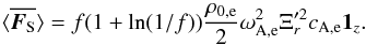 (35)Again, the flux is expressed in W/m2 and can easily be calculated. The filling factor f is available from observations. The equilibrium density outside the flux tube ρ0,e can be found in empirical models of the solar atmosphere. We use to denote the radial component of the Lagrangian displacement at the flux tube boundary, which can be quantified using the radial change of the structure under observation. The speed cA,e is the phase speed of the wave. The frequency ωA,e is the frequency of the wave.
Finally, we stress once more the applicability of these energy equations. The general energy equations are applicable for any axisymmetric magnetoaccoustic wave in a cylindrical plasma structure. In this way the energy equations can be used in all regions of the solar atmosphere, from the photosphere up to the corona.
Online material
Appendix A: Energy in slow wave modes in thin flux tubes
We now focus on the energy expressions for slow waves in thin flux tubes, i.e. with a small but non-zero value of kR. As in Sect. 3.1 we find that as kR → 0 the frequency of slow modes is given by ω = ωT,i ± (kR)2ln(kR)ω1, where the “plus” is the fundamental body mode and the “minus” is the surface mode. We have the same expressions for niR, κeR, and ω1 as in Sect. 3.1 and so we do not list them here. To calculate the amplitudes Ai and Ae we take some extra terms from the Bessel function expansions into account. We know that ![Mathematical equation: \appendix \setcounter{section}{1} \begin{eqnarray*} A_\mathrm{i} &=& (kR)\ln(kR)\left(- 2 {\rm i}\rho_{0\mathrm{,i}}\omega_{\mathrm{T,i}}\omega_1(1+c_{\mathrm{A,i}}^2/c_{\mathrm{s,i}}^2)\right)\left(1\mp\frac{(n_\mathrm{i}R)^2}{2}\right) R\Xi_z', \\[2mm] A_\mathrm{e} &=& A_\mathrm{i}\frac{\rho_{0\mathrm{,e}}}{\rho_{0\mathrm{,i}}}\frac{\left(\omega_{\mathrm{T,i}}^2-\omega_{\mathrm{A,e}}^2\right)}{\left(\omega_{\mathrm{T,i}}^2-\omega_{\mathrm{A,i}}^2\right)}\frac{n_\mathrm{i}R}{\kappa_\mathrm{e}R}\frac{J_1(n_\mathrm{i}R)}{K_1(\kappa_\mathrm{e}R)} \\[2mm] &=& i \frac{\rho_{0\mathrm{,e}}}{2}\frac{\left(\omega_{\mathrm{s,i}}^2-\omega_{\mathrm{T,i}}^2\right)\left(\omega_{\mathrm{T,i}}^2-\omega_{\mathrm{A,e}}^2\right)}{\omega_{\mathrm{s,i}}^2}R\Xi_z' (kR)\left(1-\frac{\left(n_\mathrm{i}R\right)^2}{8}+\frac{\left(\kappa_\mathrm{e}R\right)^2}{8}\right), \end{eqnarray*}](/articles/aa/full_html/2015/06/aa25468-14/aa25468-14-eq196.png) where there are some extra terms from the Bessel function expansions. In the first line the “plus” indicates surface modes, while the “minus” indicates the fundamental body mode. To calculate the energy inside the flux tube (Eqs. (15)and (17)) we also need to approximate some products of Bessel functions, i.e.
where there are some extra terms from the Bessel function expansions. In the first line the “plus” indicates surface modes, while the “minus” indicates the fundamental body mode. To calculate the energy inside the flux tube (Eqs. (15)and (17)) we also need to approximate some products of Bessel functions, i.e. ![Mathematical equation: \appendix \setcounter{section}{1} \begin{eqnarray*} J_0(n_{\mathrm{i}}R)^2+J_1(n_{\mathrm{i}}R)^2 &= &1 \mp \frac{\left(n_\mathrm{i}R\right)^2}{4} \\[2mm] J_1(n_{\mathrm{i}}R)^2-J_0(n_{\mathrm{i}}R)J_2(n_{\mathrm{i}}R) &=& \frac{\left(n_\mathrm{i}R\right)^2}{8} \\[2mm] K_1(\kappa_{\mathrm{e}}R)^2-K_0(\kappa_{\mathrm{e}}R)^2 &=& \frac{1}{\left(\kappa_\mathrm{e}R\right)^2} \\[2mm] K_0(\kappa_{\mathrm{e}}R)K_2(\kappa_{\mathrm{e}}R)-K_1(\kappa_{\mathrm{e}}R)^2 &=& \frac{-\ln\{\left(\kappa_\mathrm{e}R\right)^2/4\}}{\left(\kappa_\mathrm{e}R\right)^2} \approx \frac{-\ln\!\left(kR\right)}{\left(\kappa_\mathrm{e}R\right)^2}\cdot \end{eqnarray*}](/articles/aa/full_html/2015/06/aa25468-14/aa25468-14-eq197.png) In the first line the “minus” indicates the fundamental body mode, while the “plus” indicates surface modes. These expansion can all be checked in Abramowitz & Stegun (1972). We now have all the ingredients needed to calculate the energy in slow sausage wave modes in thin flux tubes. The energy inside the flux tube is given by
In the first line the “minus” indicates the fundamental body mode, while the “plus” indicates surface modes. These expansion can all be checked in Abramowitz & Stegun (1972). We now have all the ingredients needed to calculate the energy in slow sausage wave modes in thin flux tubes. The energy inside the flux tube is given by ![Mathematical equation: \appendix \setcounter{section}{1} \begin{eqnarray} \bracs{KE}_{\mathrm{i}}&=&\frac{\rho_{0\mathrm{,i}}}{4}\omega_{\mathrm{T,i}}^2 \pi R^2 \Xi_z'^2 \left(1\mp3\frac{\rho_{0\mathrm{,i}}}{\rho_{0\mathrm{,e}}}\frac{\left(\omega_{\mathrm{A,i}}^2-\omega_{\mathrm{T,i}}^2\right)}{\left(\omega_{\mathrm{A,e}}^2-\omega_{\mathrm{T,i}}^2\right)}\frac{1}{\ln(kR)}+\frac{\omega_{\mathrm{T,i}}^4}{\omega_{\mathrm{A,i}}^4}(kR)^2\right), \nonumber\\[2mm] \bracs{ME}_{\mathrm{i}}&=&\frac{\rho_{0\mathrm{,i}}}{4}\omega_{\mathrm{T,i}}^2 \pi R^2 \Xi_z'^2\frac{\omega_{\mathrm{T,i}}^2}{\omega_{\mathrm{A,i}}^2}\left(1\mp3\frac{\rho_{0\mathrm{,i}}}{\rho_{0\mathrm{,e}}}\frac{\left(\omega_{\mathrm{A,i}}^2-\omega_{\mathrm{T,i}}^2\right)}{\left(\omega_{\mathrm{A,e}}^2-\omega_{\mathrm{T,i}}^2\right)}\frac{1}{\ln(kR)}+\frac{\omega_{\mathrm{T,i}}^2}{\omega_{\mathrm{A,i}}^2}(kR)^2\right), \nonumber\\[2mm] \bracs{IE}_{\mathrm{i}}&=&\frac{\rho_{0\mathrm{,i}}}{4}\omega_{\mathrm{T,i}}^2 \pi R^2 \Xi_z'^2\frac{\omega_{\mathrm{T,i}}^2}{\omega_{\mathrm{s,i}}^2}\left(1\mp3\frac{\rho_{0\mathrm{,i}}}{\rho_{0\mathrm{,e}}}\frac{\left(\omega_{\mathrm{A,i}}^2-\omega_{\mathrm{T,i}}^2\right)}{\left(\omega_{\mathrm{A,e}}^2-\omega_{\mathrm{T,i}}^2\right)}\frac{1}{\ln(kR)}\right), \nonumber\\[2mm] \bracs{TE}_{\mathrm{i}}&=&\frac{\rho_{0\mathrm{,i}}}{2}\omega_{\mathrm{T,i}}^2 \pi R^2 \Xi_z'^2\left(1\mp3\frac{\rho_{0\mathrm{,i}}}{\rho_{0\mathrm{,e}}}\frac{\left(\omega_{\mathrm{A,i}}^2-\omega_{\mathrm{T,i}}^2\right)}{\left(\omega_{\mathrm{A,e}}^2-\omega_{\mathrm{T,i}}^2\right)}\frac{1}{\ln(kR)}+\frac{\omega_{\mathrm{T,i}}^4}{\omega_{\mathrm{A,i}}^4}(kR)^2\right), \nonumber\\[2mm] \bracs{\vec{S}}_{\mathrm{i}}&=&\frac{\rho_{0\mathrm{,i}}}{2}\omega_{\mathrm{T,i}}^2 \pi R^2 \Xi_z'^2 c_{\mathrm{T,i}}\frac{\omega_{\mathrm{T,i}}^2}{\omega_{\mathrm{A,i}}^2}(kR)^2 \vec{1_{\textit{z}}}, \nonumber\\[2mm] \bracs{\vec{T}}_{\mathrm{i}}&=&\frac{\rho_{0\mathrm{,i}}}{2}\omega_{\mathrm{T,i}}^2 \pi R^2 \Xi_z'^2 c_{\mathrm{T,i}}\left(1\mp3\frac{\rho_{0\mathrm{,i}}}{\rho_{0\mathrm{,e}}}\frac{\left(\omega_{\mathrm{A,i}}^2-\omega_{\mathrm{T,i}}^2\right)}{\left(\omega_{\mathrm{A,e}}^2-\omega_{\mathrm{T,i}}^2\right)}\frac{1}{\ln(kR)}\right) \vec{1_{\textit{z}}}, \nonumber\\[2mm] \bracs{\vec{E}}_{\mathrm{i}}&=&\frac{\rho_{0\mathrm{,i}}}{2}\omega_{\mathrm{T,i}}^2 \pi R^2 \Xi_z'^2 c_{\mathrm{T,i}}\left(1\mp3\frac{\rho_{0\mathrm{,i}}}{\rho_{0\mathrm{,e}}}\frac{\left(\omega_{\mathrm{A,i}}^2-\omega_{\mathrm{T,i}}^2\right)}{\left(\omega_{\mathrm{A,e}}^2-\omega_{\mathrm{T,i}}^2\right)}\frac{1}{\ln(kR)}+\frac{\omega_{\mathrm{T,i}}^2}{\omega_{\mathrm{A,i}}^2}(kR)^2\right) \vec{1_{\textit{z}}} \label{eq:slow_mode_internal}, \end{eqnarray}](/articles/aa/full_html/2015/06/aa25468-14/aa25468-14-eq198.png) (A.1)where we have kept all terms of order (kR)2 or lower. The “minus” indicates the fundamental body mode, while the “plus” indicates surface modes. We notice the equipartition between kinetic and potential (i.e. the sum of both magnetic and thermal energy) energy. The energy outside the flux tube (Eqs. (19)) can also be calculated and we find
(A.1)where we have kept all terms of order (kR)2 or lower. The “minus” indicates the fundamental body mode, while the “plus” indicates surface modes. We notice the equipartition between kinetic and potential (i.e. the sum of both magnetic and thermal energy) energy. The energy outside the flux tube (Eqs. (19)) can also be calculated and we find ![Mathematical equation: \appendix \setcounter{section}{1} \begin{eqnarray} \bracs{KE}_{\mathrm{e}}&=&\frac{\rho_{0\mathrm{,e}}}{4}\omega_{\mathrm{T,i}}^2 \pi R^2 \Xi_z'^2 \frac{1}{4}\frac{\omega_{\mathrm{T,i}}^2}{\omega_{\mathrm{A,i}}^2}\left((kR)^2\left(-\ln(kR)\right)+\left(\frac{1}{2}\frac{\rho_{0\mathrm{,i}}}{\rho_{0\mathrm{,e}}}\frac{\omega_{\mathrm{T,i}}^2}{\left(\omega_{\mathrm{A,e}}^2-\omega_{\mathrm{T,i}}^2\right)}\frac{\omega_{\mathrm{A,i}}^2}{\omega_{\mathrm{s,i}}^2}+\frac{\omega_{\mathrm{T,i}}^2}{\omega_{\mathrm{A,i}}^2}\frac{\omega_{\mathrm{T,e}}^4}{\omega_{\mathrm{A,e}}^4}\frac{\left(\omega_{\mathrm{s,e}}^2+\omega_{\mathrm{A,e}}^2\right)\left(\omega_{\mathrm{A,e}}^2-\omega_{\mathrm{T,i}}^2\right)}{\left(\omega_{\mathrm{s,e}}^2-\omega_{\mathrm{T,i}}^2\right)\left(\omega_{\mathrm{T,e}}^2-\omega_{\mathrm{T,i}}^2\right)}\right)(kR)^2\right), \nonumber\\[2mm] \bracs{ME}_{\mathrm{e}}&=&\frac{\rho_{0\mathrm{,e}}}{4}\omega_{\mathrm{T,i}}^2 \pi R^2 \Xi_z'^2 \frac{1}{4}\frac{\omega_{\mathrm{A,e}}^2}{\omega_{\mathrm{A,i}}^2}\left((kR)^2\left(-\ln(kR)\right)+\left(\frac{1}{2}\frac{\rho_{0\mathrm{,i}}}{\rho_{0\mathrm{,e}}}\frac{\omega_{\mathrm{T,i}}^2}{\left(\omega_{\mathrm{A,e}}^2-\omega_{\mathrm{T,i}}^2\right)}\frac{\omega_{\mathrm{A,i}}^2}{\omega_{\mathrm{s,i}}^2}+\frac{\omega_{\mathrm{T,i}}^2}{\omega_{\mathrm{A,i}}^2}\frac{\left(\omega_{\mathrm{s,e}}^2-\omega_{\mathrm{T,i}}^2\right)\left(\omega_{\mathrm{A,e}}^2-\omega_{\mathrm{T,i}}^2\right)}{\left(\omega_{\mathrm{s,e}}^2+\omega_{\mathrm{A,e}}^2\right)\left(\omega_{\mathrm{T,e}}^2-\omega_{\mathrm{T,i}}^2\right)}\right)(kR)^2\right), \nonumber\\[2mm] \bracs{IE}_{\mathrm{e}}&=&\frac{\rho_{0\mathrm{,e}}}{4}\omega_{\mathrm{T,i}}^2 \pi R^2 \Xi_z'^2 \frac{1}{4}\frac{\omega_{\mathrm{T,i}}^2}{\omega_{\mathrm{s,e}}^2}\frac{\omega_{\mathrm{T,i}}^4}{\omega_{\mathrm{A,i}}^4}\frac{\omega_{\mathrm{T,e}}^4}{\omega_{\mathrm{A,e}}^4}\frac{\left(\omega_{\mathrm{s,e}}^2+\omega_{\mathrm{A,e}}^2\right)\left(\omega_{\mathrm{A,e}}^2-\omega_{\mathrm{T,i}}^2\right)}{\left(\omega_{\mathrm{s,e}}^2-\omega_{\mathrm{T,i}}^2\right)\left(\omega_{\mathrm{T,e}}^2-\omega_{\mathrm{T,i}}^2\right)} (kR)^2, \nonumber\\[2mm] \bracs{TE}_{\mathrm{e}}&=&\bracs{KE}_{\mathrm{e}}+\bracs{ME}_{\mathrm{e}}+\bracs{IE}_{\mathrm{e}}, \nonumber\\[2mm] \bracs{\vec{S}}_{\mathrm{e}}&=&\frac{\rho_{0\mathrm{,e}}}{2}\omega_{\mathrm{T,i}}^2 \pi R^2 \Xi_z'^2 c_{\mathrm{T,i}} \frac{1}{4} \left((kR)^2\left(-\ln(kR)\right)+\left(\frac{1}{2}\frac{\rho_{0\mathrm{,i}}}{\rho_{0\mathrm{,e}}}\frac{\omega_{\mathrm{T,i}}^2}{\left(\omega_{\mathrm{A,e}}^2-\omega_{\mathrm{T,i}}^2\right)}\frac{\omega_{\mathrm{A,i}}^2}{\omega_{\mathrm{s,i}}^2}+\frac{\omega_{\mathrm{T,i}}^2}{\omega_{\mathrm{A,i}}^2}\frac{\omega_{\mathrm{T,e}}^4}{\omega_{\mathrm{A,e}}^4}\frac{\left(\omega_{\mathrm{s,e}}^2+\omega_{\mathrm{A,e}}^2\right)\left(\omega_{\mathrm{A,e}}^2-\omega_{\mathrm{T,i}}^2\right)}{\left(\omega_{\mathrm{s,e}}^2-\omega_{\mathrm{T,i}}^2\right)\left(\omega_{\mathrm{T,e}}^2-\omega_{\mathrm{T,i}}^2\right)}\right)(kR)^2\right) \vec{1_{\textit{z}}}, \nonumber\\[2mm] \bracs{\vec{T}}_{\mathrm{e}}&=&\frac{\rho_{0\mathrm{,e}}}{2}\omega_{\mathrm{T,i}}^2 \pi R^2 \Xi_z'^2 c_{\mathrm{T,i}} \frac{1}{4}\frac{\omega_{\mathrm{T,i}}^4}{\omega_{\mathrm{A,i}}^4}\frac{\omega_{\mathrm{T,e}}^4}{\omega_{\mathrm{A,e}}^4}\frac{\left(\omega_{\mathrm{s,e}}^2+\omega_{\mathrm{A,e}}^2\right)\left(\omega_{\mathrm{A,e}}^2-\omega_{\mathrm{T,i}}^2\right)}{\left(\omega_{\mathrm{s,e}}^2-\omega_{\mathrm{T,i}}^2\right)\left(\omega_{\mathrm{T,e}}^2-\omega_{\mathrm{T,i}}^2\right)} (kR)^2 \vec{1_{\textit{z}}}, \nonumber\\[2mm] \bracs{\vec{E}}_{\mathrm{e}}&=& \bracs{\vec{S}}_{\mathrm{e}}+\bracs{\vec{T}}_{\mathrm{e}}\label{eq:slow_mode_external}, \end{eqnarray}](/articles/aa/full_html/2015/06/aa25468-14/aa25468-14-eq200.png) (A.2)where again we have kept all terms of order (kR)2 or lower. The dominant term in these energy equations is the (kR)2( − ln(kR)) term. This shows that we do not find equipartition in this case since the coefficients in the kinetic and magnetic energy before the (kR)2( − ln(kR)) term are not the same. This puzzling result was further investigated numerically. We used different equilibrium parameters with different small values of kR. We discovered a small error in the equipartition of energy of the order of 10-5 of the total energy. When using the full set of equations to calculate the energy (i.e. Eqs. (17)and (19)) we did find equipartition between kinetic and potential energy. This clearly shows that there is indeed equipartition, but approximating the Bessel functions has introduced a small error.
(A.2)where again we have kept all terms of order (kR)2 or lower. The dominant term in these energy equations is the (kR)2( − ln(kR)) term. This shows that we do not find equipartition in this case since the coefficients in the kinetic and magnetic energy before the (kR)2( − ln(kR)) term are not the same. This puzzling result was further investigated numerically. We used different equilibrium parameters with different small values of kR. We discovered a small error in the equipartition of energy of the order of 10-5 of the total energy. When using the full set of equations to calculate the energy (i.e. Eqs. (17)and (19)) we did find equipartition between kinetic and potential energy. This clearly shows that there is indeed equipartition, but approximating the Bessel functions has introduced a small error.
When taking the long wavelength limit (i.e. kR = 0) we find that Eqs. (A.1)and (A.2)simplify to Eqs. (24)as expected.
Acknowledgments
We have received funding from the Odysseus programme of the FWO-Vlaanderen. The research was conducted in the framework of Belspo’s IAP P7/08 CHARM and the GOA-2015-014 of the Research Council of the KU Leuven. D.B.J. wishes to thank STFC for the award of an Ernest Rutherford Fellowship alongside a dedicated Research Grant. S.D.T.G. thanks the Northern Ireland Department for Employment and Learning for a Ph.D. studentship.
References
- Abramowitz, M., & Stegun, I. A. 1972, Handbook of Mathematical Functions, eds. M. Abramowitz, &, I. A. Stegun [Google Scholar]
- Andries, J., & Cally, P. S. 2011, ApJ, 743, 164 [NASA ADS] [CrossRef] [Google Scholar]
- Andries, J., Arregui, I., & Goossens, M. 2005, ApJ, 624, L57 [NASA ADS] [CrossRef] [Google Scholar]
- Andries, J., Van Doorsselaere, T., Roberts, B., et al. 2009, Space Sci. Rev., 149, 3 [NASA ADS] [CrossRef] [Google Scholar]
- Aschwanden, M. J., & Schrijver, C. J. 2011, ApJ, 736, 102 [NASA ADS] [CrossRef] [Google Scholar]
- Aschwanden, M. J., Nakariakov, V. M., & Melnikov, V. F. 2004, ApJ, 600, 458 [NASA ADS] [CrossRef] [Google Scholar]
- Banerjee, D., Erdélyi, R., Oliver, R., & O’Shea, E. 2007, Sol. Phys., 246, 3 [NASA ADS] [CrossRef] [Google Scholar]
- Banerjee, D., Pérez-Suárez, D., & Doyle, J. G. 2009, A&A, 501, L15 [NASA ADS] [CrossRef] [EDP Sciences] [Google Scholar]
- Beckers, J. M., & Schultz, R. B. 1972, Sol. Phys., 27, 61 [NASA ADS] [CrossRef] [Google Scholar]
- Bharti, L., Jain, R., Joshi, C., & Jaaffrey, S. N. A. 2006, in Solar MHD Theory and Observations: A High Spatial Resolution Perspective, eds. J. Leibacher, R. F. Stein, & H. Uitenbroek, ASP Conf. Ser., 354, 13 [Google Scholar]
- Bhatnagar, A. 1971, Sol. Phys., 18, 40 [NASA ADS] [CrossRef] [Google Scholar]
- Cally, P. S. 1986, Sol. Phys., 103, 277 [NASA ADS] [CrossRef] [Google Scholar]
- Collados, M., Bettonvil, F., Cavaller, L., et al. 2010, in SPIE Conf. Ser., 7733 [Google Scholar]
- De Moortel, I. 2009, Space Sci. Rev., 149, 65 [NASA ADS] [CrossRef] [Google Scholar]
- De Moortel, I., & Nakariakov, V. M. 2012, Roy. Soc. London Philos. Trans. Ser. A, 370, 3193 [Google Scholar]
- De Moortel, I., Ireland, J., & Walsh, R. W. 2000, A&A, 355, L23 [NASA ADS] [Google Scholar]
- De Pontieu, B., McIntosh, S. W., Carlsson, M., et al. 2007, Science, 318, 1574 [NASA ADS] [CrossRef] [PubMed] [Google Scholar]
- Dorotovič, I., Erdélyi, R., & Karlovský, V. 2008, Waves and Oscillations in the Solar Atmosphere: Heating and Magneto-Seismology, eds. R. Erdélyi, & C. A. Mendoza-Briceno, IAU Symp., 247, 351 [Google Scholar]
- Dorotovič, I., Erdélyi, R., Freij, N., Karlovský, V., & Márquez, I. 2014, A&A, 563, A12 [NASA ADS] [CrossRef] [EDP Sciences] [Google Scholar]
- Edwin, P. M., & Roberts, B. 1983, Sol. Phys., 88, 179 [NASA ADS] [CrossRef] [Google Scholar]
- Elmore, D. F., Rimmele, T., Casini, R., et al. 2014, SPIE Conf. Ser., 9147, 7 [Google Scholar]
- Erdélyi, R. 2004, A&G, 45, 34 [Google Scholar]
- Goossens, M., Van Doorsselaere, T., Soler, R., & Verth, G. 2013a, ApJ, 768, 191 [NASA ADS] [CrossRef] [Google Scholar]
- Goossens, M., Van Doorsselaere, T., Soler, R., & Verth, G. 2013b, ApJ, 771, 74 [NASA ADS] [CrossRef] [Google Scholar]
- Jess, D. B., Mathioudakis, M., Erdélyi, R., et al. 2009, Science, 323, 1582 [NASA ADS] [CrossRef] [PubMed] [Google Scholar]
- Jess, D. B., Mathioudakis, M., Christian, D. J., et al. 2010, Sol. Phys., 261, 363 [NASA ADS] [CrossRef] [Google Scholar]
- Jess, D. B., Reznikova, V. E., Van Doorsselaere, T., Keys, P. H., & Mackay, D. H. 2013, ApJ, 779, 168 [NASA ADS] [CrossRef] [Google Scholar]
- Krishna Prasad, S., Banerjee, D., Van Doorsselaere, T., & Singh, J. 2012, A&A, 546, A50 [NASA ADS] [CrossRef] [EDP Sciences] [Google Scholar]
- Martínez González, M. J., Asensio Ramos, A., Manso Sainz, R., et al. 2011, ApJ, 730, L37 [NASA ADS] [CrossRef] [Google Scholar]
- McAteer, R. T. J., Gallagher, P. T., Williams, D. R., et al. 2003, ApJ, 587, 806 [NASA ADS] [CrossRef] [Google Scholar]
- Melnikov, V. F., Reznikova, V. E., Shibasaki, K., & Nakariakov, V. M. 2005, A&A, 439, 727 [NASA ADS] [CrossRef] [EDP Sciences] [Google Scholar]
- Moreels, M. G., & Van Doorsselaere, T. 2013, A&A, 551, A137 [NASA ADS] [CrossRef] [EDP Sciences] [Google Scholar]
- Moreels, M. G., Goossens, M., & Van Doorsselaere, T. 2013, A&A, 555, A75 [NASA ADS] [CrossRef] [EDP Sciences] [Google Scholar]
- Moreels, M. G., Freij, N., Erdélyi, R., Van Doorsselaere, T., & Verth, G. 2015, A&A, submitted [Google Scholar]
- Morton, R. J., Erdélyi, R., Jess, D. B., & Mathioudakis, M. 2011, ApJ, 729, L18 [NASA ADS] [CrossRef] [Google Scholar]
- Morton, R. J., Verth, G., Jess, D. B., et al. 2012a, Nature Comm., 3, 1315 [Google Scholar]
- Morton, R. J., Verth, G., McLaughlin, J. A., & Erdélyi, R. 2012b, ApJ, 744, 5 [NASA ADS] [CrossRef] [Google Scholar]
- Morton, R. J., Verth, G., Hillier, A., & Erdélyi, R. 2014, ApJ, 784, 29 [NASA ADS] [CrossRef] [Google Scholar]
- Nakariakov, V. M., Melnikov, V. F., & Reznikova, V. E. 2003, A&A, 412, L7 [NASA ADS] [CrossRef] [EDP Sciences] [Google Scholar]
- Ofman, L. 2005, Space Sci. Rev., 120, 67 [NASA ADS] [CrossRef] [Google Scholar]
- Roberts, P. H., & Boardman, A. D. 1962, ApJ, 135, 552 [NASA ADS] [CrossRef] [Google Scholar]
- Sakurai, T., Goossens, M., & Hollweg, J. V. 1991, Sol. Phys., 133, 227 [NASA ADS] [CrossRef] [Google Scholar]
- Thompson, B. J., Gurman, J. B., Neupert, W. M., et al. 1999, ApJ, 517, L151 [NASA ADS] [CrossRef] [Google Scholar]
- Thurgood, J. O., Morton, R. J., & McLaughlin, J. A. 2014, ApJ, 790, L2 [NASA ADS] [CrossRef] [Google Scholar]
- Tomczyk, S., McIntosh, S. W., Keil, S. L., et al. 2007, Science, 317, 1192 [NASA ADS] [CrossRef] [PubMed] [Google Scholar]
- Van Doorsselaere, T., Andries, J., Poedts, S., & Goossens, M. 2004a, ApJ, 606, 1223 [NASA ADS] [CrossRef] [Google Scholar]
- Van Doorsselaere, T., Debosscher, A., Andries, J., & Poedts, S. 2004b, A&A, 424, 1065 [NASA ADS] [CrossRef] [EDP Sciences] [Google Scholar]
- Van Doorsselaere, T., Nakariakov, V. M., & Verwichte, E. 2008, ApJ, 676, L73 [NASA ADS] [CrossRef] [Google Scholar]
- Van Doorsselaere, T., De Groof, A., Zender, J., Berghmans, D., & Goossens, M. 2011, ApJ, 740, 90 [NASA ADS] [CrossRef] [Google Scholar]
- Van Doorsselaere, T., Gijsen, S. E., Andries, J., & Verth, G. 2014, ApJ, 795, 18 [NASA ADS] [CrossRef] [Google Scholar]
- Vasheghani Farahani, S., Hornsey, C., Van Doorsselaere, T., & Goossens, M. 2014, ApJ, 781, 92 [NASA ADS] [CrossRef] [Google Scholar]
- Verwichte, E., Foullon, C., & Nakariakov, V. M. 2006, A&A, 446, 1139 [NASA ADS] [CrossRef] [EDP Sciences] [Google Scholar]
- Walker, A. 2005, Magnetohydrodynamic Waves in Geospace: The Theory of Ulf Waves and Their Interaction with Energetic Particles in the Solar-Terrestrial Environment [Google Scholar]
- Walsh, R. W., & Ireland, J. 2003, A&ARv, 12, 1 [Google Scholar]
- Wang, T., Solanki, S. K., Curdt, W., Innes, D. E., & Dammasch, I. E. 2002, ApJ, 574, L101 [NASA ADS] [CrossRef] [Google Scholar]
- Wang, T. J., Solanki, S. K., Innes, D. E., Curdt, W., & Marsch, E. 2003, A&A, 402, L17 [NASA ADS] [CrossRef] [EDP Sciences] [Google Scholar]
- Yuan, D., Sych, R., Reznikova, V. E., & Nakariakov, V. M. 2014, A&A, 561, A19 [NASA ADS] [CrossRef] [EDP Sciences] [Google Scholar]
- Zaitsev, V. V., & Stepanov, A. V. 1975, Issled. Geomagn. Aeron. Fiz. Solntsa, 3 [Google Scholar]
All Figures
|
Fig. 1 Equilibrium configuration of the flux tube. |
| In the text | |
|
Fig. 2 Phase speed diagram of wave modes under photospheric conditions. We have taken cA,i = 2cs,i, cA,e = 0.5cs,i, and cs,e = 1.5cs,i. The Alfvén speeds are not indicated in the graph because no modes with real frequencies appear in that vicinity. The modes with phase speeds between cT,i and cs,i are body modes and the other modes are surface modes. We note that we only plotted two body modes, while there are infinitely many radial overtones. |
| In the text | |
|
Fig. 3 Phase speed diagram of wave modes under coronal conditions. We have taken cA,i = 2cs,i, cA,e = 5cs,i, and cs,e = 0.5cs,i. All modes are body modes. For the slow modes we only plotted one mode, for the fast modes we plotted five modes, while for both there are an infinite number of radial overtones. |
| In the text | |
Current usage metrics show cumulative count of Article Views (full-text article views including HTML views, PDF and ePub downloads, according to the available data) and Abstracts Views on Vision4Press platform.
Data correspond to usage on the plateform after 2015. The current usage metrics is available 48-96 hours after online publication and is updated daily on week days.
Initial download of the metrics may take a while.