| Issue |
A&A
Volume 578, June 2015
|
|
|---|---|---|
| Article Number | A23 | |
| Number of page(s) | 16 | |
| Section | Interstellar and circumstellar matter | |
| DOI | https://doi.org/10.1051/0004-6361/201424073 | |
| Published online | 29 May 2015 | |
Identification of new transitional disk candidates in Lupus with Herschel⋆,⋆⋆
1 European Space Astronomy Centre (ESA), PO Box, 78, 28691 Villanueva de la Cañada, Madrid, Spain
e-mail: This email address is being protected from spambots. You need JavaScript enabled to view it.
2 Centro de Astrobiología, INTA-CSIC, PO Box – Apdo. de correos 78, 28691 Villanueva de la Cañada Madrid, Spain
3 ISDEFE – ESAC, PO Box 78, 28691 Villanueva de la Cañada, Madrid, Spain
4 ESA Science Support Office, ESTEC/SRE-S, Keplerlaan 1, 2201 AZ Noordwijk, The Netherlands
5 Laboratoire AIM Paris, Saclay, CEA/DSM, CNRS, Université Paris Diderot, IRFU, Service d’Astrophysique, Centre d’Études de Saclay, Orme des Merisiers, 91191 Gif-sur-Yvette, France
Received: 25 April 2014
Accepted: 15 January 2015
Abstract
Context. New data from the Herschel Space Observatory are broadening our understanding of the physics and evolution of the outer regions of protoplanetary disks in star-forming regions. In particular they prove to be useful for identifying transitional disk candidates.
Aims. The goals of this work are to complement the detections of disks and the identification of transitional disk candidates in the Lupus clouds with data from the Herschel Gould Belt Survey.
Methods. We extracted photometry at 70, 100, 160, 250, 350, and 500 μm of all spectroscopically confirmed Class II members previously identified in the Lupus regions and analyzed their updated spectral energy distributions.
Results. We have detected 34 young disks in Lupus in at least one Herschel band, from an initial sample of 123 known members in the observed fields. Using recently defined criteria, we have identified five transitional disk candidates in the region. Three of them are new to the literature. Their PACS-70 μm fluxes are systematically higher than those of normal T Tauri stars in the same associations, as already found in T Cha and in the transitional disks in the Chamaeleon molecular cloud.
Conclusions. Herschel efficiently complements mid-infrared surveys for identifying transitional disk candidates and confirms that these objects seem to have substantially different outer disks than the T Tauri stars in the same molecular clouds.
Key words: stars: pre-main sequence / protoplanetary disks / planetary systems
Herschel is an ESA space observatory with science instruments provided by European-led Principal Investigator consortia and with important participation from NASA.
Tables 5–7 and Figs. 3 and 4 are available in electronic form at http://www.aanda.org
© ESO, 2015
1. Introduction
Transitional disks link the studies of planet formation and disk evolution around young stars. They are protoplanetary disks around young stars, optically thick and gas rich, with astronomical unit-scale inner disk clearings or radial gaps evident in their spectral energy distributions (SEDs). They lack excess emission at short-mid infrared (typically around 8–12 μm), but present considerable emission at longer wavelengths (Muzerolle et al. 2010). Since their discovery by Strom et al. (1989) with IRAS data, the Spitzer Space Telescope (Werner et al. 2004) allowed the identification of a much larger population of these objects (Cieza et al. 2010; Merín et al. 2010; Espaillat et al. 2014). It was possible to use the mid-infrared data to make good estimates of the dust distribution in the inner few astronomical units of the disks around T Tauri stars in nearby star-forming regions (e.g. Calvet et al. 2005; Lada et al. 2006).
The Herschel Space Observatory (Pilbratt et al. 2010) grants us access to the outer disk region of these objects. Recent studies suggest that the outer disks, as detected in far-infrared emission, undergo substantial transformations in the transitional disk phase (Cieza et al. 2011; Ribas et al. 2013). However, Herschel data are still lacking for most known transitional disks.
The main objective of this article is to revisit and extend our knowledge of known Class II objects in the Lupus dark clouds, and to identify transitional disk candidates in the region using Herschel photometry, complemented with photometry from previous studies from the optical to the mid-infrared. With Herschel we have the opportunity to study objects with large inner holes, reaching the farthest regions of their disks that Spitzer was unable to access with the required sensitivity (IRAC and IRS had different wavelength ranges, 3.5–8.0 μm and 5–35 μm, respectively, and the sensitivity of MIPS, with pass bands between 24 and 160 μm, was limited). Therefore, we are not only able to study the outer regions of known transitional disks, but also to detect new candidates, with larger cavities and outer disks.
This work is organized as follows. Section 2 describes the Herschel observations and data reduction and the procedure applied to identify and extract the fluxes for the known objects. In Sect. 3 we identify new transitional disk candidates, describe the procedure to build the SEDs, and discuss some objects with certain peculiarities. In Sect. 4 we discuss the properties of the newly found transitional disk candidates, and in Sect. 5 we present the conclusions of this work.
2. Observations and data reduction
The Lupus dark clouds were observed by Herschel as part of the Herschel Gould Belt Survey (HGBS; André et al. 2010). It is one of the star-forming regions located within 150 to 200 pc from the Sun and has a mean age of a few Myr (see Comerón 2008, for a review of the region). It contains four main regions, with one of them, Lupus III, being a rich T Tauri association. Located in the Scorpius-Centaurus OB association, the massive stars in the region are likely to have played a significant role in its evolution.
By employing the PACS (Poglitsch et al. 2010) and SPIRE (Griffin et al. 2010) photometers in parallel mode, Herschel has the capability for large scale mapping of star-forming regions in the far-infrared range. Early Herschel observations of Lupus from the HGBS were already published by Rygl et al. (2013), where the observing strategy and main results are described.
We produced our maps using Scanamorphos (Roussel 2012) version 21.0 for the PACS maps and version 18.0 for the SPIRE maps. The identification numbers of the Lupus Herschel parallel mode observations processed for this work are (1342-)189880, 189881, 203070, 2203071, 2203087, 2203088, 2213182, and 2213183 from program KPGT_pandre_1. The observations were made in parallel mode for 70, 160, 250, 350, and 500 μm, and in prime mode for 100 μm (Rygl et al. 2013), which is why some of the sources do not have images at 100 μm in Fig. 4.
A complete census of the sources detected with Herschel will be published by the HGBS consortium in an upcoming paper (Benedettini et al., in prep.).
2.1. Point source photometry
Our first objective was to detect and classify sources in the images obtained with PACS and SPIRE. We used coordinates of spectroscopically confirmed Class II members from different sources, compiling a list of 217 targets. This compilation was developed by Ribas et al. (2014), and these objects were selected for having known extinction values and spectral types from optical spectroscopy. Of this sample of 217 objects, only 123 are found in the fields observed by Herschel.
We applied the sourceExtractorSussextractor algorithm in our maps, with the Herschel interactive processing environment (HIPE), version 12.0, using a detection threshold of S/N> 3. We then cross-matched the resulting list of detected objects with our pre-selected targets, using a search radius between 5′′ and 10′′. We selected only those objects with detections in PACS. After this process, we found 37 objects with at least one detection in one PACS band, 35 in the 70 μm maps, and 2 in the 100 μm maps. We then validated all of them by visual inspection. This way we were able to double-check our detections. The background emission becomes more significant at longer wavelengths, where detections are in general less frequent, or false detections appear, due to bright filaments and ridges. This is the reason why we selected only PACS-detected objects. The combination of quantitative and qualitative analysis was essential to produce reliable detections and photometry. After this process we discarded four objects as not having clear detections in the maps and added two objects that were found by visual inspection. They are flagged in Table 5. After this process, 35 objects in the list had one clean detection in at least one Herschel PACS or SPIRE band.
We applied the sourceExtractorDaophot algorithm to extract the photometry for PACS, and the annularSkyAperturePhotometry task for SPIRE. All point-source fluxes were aperture corrected with the recommended aperture corrections for both instruments (see the PACS photometer point spread function technical note from April 2012, and Sect. 6.7.1 of the SPIRE Data Reduction Guide of HIPE 12.0). Table 1 shows the set of aperture, inner, and outer sky radii for each Herschel band, as well as the corresponding aperture corrections.
Aperture, inner, and outer radii used in the photometry extraction process for each band, with their corresponding aperture corrections.
Table 2 shows the sensitivity limit for each Herschel band, as stated in the SPIRE/PACS Parallel Mode Observers’ Manual (Sect. 2.3). The values correspond to a nominal scan direction and a scan speed of 60′′/s.
Sensitivity limits for each Herschel band in parallel mode at 60′′/s, as stated in the PACS/SPIRE Parallel Mode Observers’ Manual.
Upper limits for non-detections were derived by adding scaled synthetic point spread functions (PSFs) at the expected position of the sources until the sussExtractor detection algorithm did not recover them. In most cases visual inspection was applied. The calibration errors for PACS and SPIRE are 5% and 7% (as stated in their observer manuals), respectively. To ensure consistency with Ribas et al. (2013) we chose a more conservative estimation, 20% for SPIRE as error values, taking into account that the background emission becomes increasingly stronger at longer wavelengths. In the case of PACS, after comparing several photometric extraction algorithms (sussExtractor, Daophot, annularSkyAperturePhotometry, and Hyper, Traficante et al. 2015), and extraction apertures with the MIPS70 fluxes of a subsample of clean sources, we selected a conservative error value of 25% of the flux to account for the different flux values obtained. Table 5 gives the stellar parameters of these detected sources as given in the literature, and Table 6 presents their Herschel point source fluxes and upper limits. As stated before, at least one point source was detected for at least one wavelength of the Herschel instruments for all objects in Table 6 (see Fig. 4).
Targets with possible contamination within the used apertures in MIPS24.
We then looked for bright Spitzer 24 μm and 70 μm sources around the targets to check for possible contamination from other nearby mid-infrared sources. We used a radius of 42′′, as this was the value we used for the largest wavelength band when extracting the Herschel photometry (which corresponds to SPIRE 500 μm). The results of this analysis are shown in Tables 3 and 4.
In the cases where MIPS70 sources were found near our sources we inspected the PACS70 images of the targets. Except for sources Sz65, Sz66, Sz103, Sz104, and 2MASSJ1608537 (as explained below), we did not find evidence of the presence of extra sources inside the matching radius (see Fig. 4). This means that Herschel did not detect them, so we assume that the full contribution to the flux measured at PACS70 comes from our target sources, and not from contaminants. In Table 4 we maintain all the sources with possible contamination for reference.
Objects Sz65 and Sz66 form a pair, as is explained in Sect. 3.3.6, and this is taken into account in their photometry extraction. The MIPS excesses seen for objects Sz103 are associated with object Sz104, and vice versa. We only flagged objects with potential contaminations in case they were detected (see Table 6). When they are not detected and upper limits are calculated instead, we do not take into account the possible contaminations.
The nearby source near object 2MASSJ1608537 presented significantly larger MIPS24 and MIPS70 fluxes than our target. In this case, we concluded that the infrared excesses measured in the Herschel image corresponded to this other object instead of our target, and thus we discarded object 2MASSJ1608537 because its Herschel photometry could not be unequivocally associated with it. The other object is a known young stellar object (YSO) candidate, SSTc2d J160853.2-391440. It is probably another member of the Lupus region, yet not confirmed spectroscopically and therefore not included in our study.
In other cases other contaminant sources were found, but with sufficiently weaker MIPS24 and MIPS70 fluxes so as not to affect our measurements. These sources are marked in Table 3. In these cases we assumed that the Herschel fluxes measured correspond to our targets as the major contributors.
Another interesting object is Sz108B, which presents two possible contaminants that could affect its photometry. The one farthest away, at 38.8′′, has larger MIPS24 flux. The closest one, at 9.7′′, has a higher MIPS70 flux. Thus, the Herschel photometry of Sz108B could be contaminated by the closest one and therefore it is flagged as unreliable in Table 4.
After this analysis, our final set of sources decreased to 34. We maintain the image of object 2MASSJ1608537 in Fig. 4 for completeness.
3. Results
3.1. Identification of transitional disk candidates
To identify transitional disk candidates we applied the procedure developed in Ribas et al. (2013), which defines a transitional disk candidate as having αK−12< 0 and α12−70> 0, where αλ1−λ2 is defined as αλ1−λ2 =  , and λ is measured in μm and Fλ in erg s-1 cm-2.
The K-band flux comes from 2MASS (Skrutskie et al. 2006), the 12 μm flux from WISE and the 70 μm flux from PACS. Some exceptions to this rule were applied when these fluxes were unavailable for certain objects; for example, Sz95 has no flux at 70 μm, so we used PACS100 μm instead. We did the same for 2MASS J1608149. An exceptional case is object SSTc2dJ160111.6-413730, discussed later in Sect. 3.3.5, as no PACS flux was available, and therefore could not be classified.
With this procedure we detected five objects that satisfy the transitional disk candidate criteria: SSTc2dJ161029.6-392215, Sz91, Sz111, Sz123, and 2MASS J1608149. In Fig. 1 we show the objects that fulfilled our selection criteria. Objects Sz91 and Sz111 were previously known transitional disks from Spitzer data (Merín et al. 2008), and they occupy a different region in the diagram than the others. They present little to no excess at 12 μm and a steep rise between 12 and 70 μm in their SEDs (see Fig. 2). This could be indicative of a large cavity in both cases, mostly empty of small dust grains. In the case of Sz91, a resolved image of this inner hole has already been obtained in the submillimeter with SMA (Tsukagoshi et al. 2014), being one of the largest imaged so far (~65 AU) in a T Tauri disk. Sz111 is likely to have a similarly large and empty cavity.
The rest of the objects present excesses at intermediate wavelengths, and fulfill our color criteria (see Fig. 2 for a representation of their SEDs). Object 2MASS J1608149 is a special case, as is explained in Sect. 3.3.3.
In Fig. 1 three additional objects present error bars falling in the transitional disk detection criteria: SSTc2dJ160703.9-391112, RXJ1608.6-3922, and Sz108B. Their SEDs present far-infrared excesses, but mid-infrared ones as well. As they do not strictly fulfill our selection criteria, they are not to be considered transitional disk candidates in this work, yet they deserve attention.
Analysis of the remaining sample of T Tauris in the Lupus regions is outside the scope of this work, although special cases are discussed in some detail in Sect. 3.3.
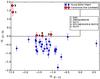 |
Fig. 1 Identification of transitional disk candidates applying the color criteria from Ribas et al. (2013) to the Lupus Herschel data. |
3.2. Spectral energy distributions
To construct the SEDs we used ancillary data from ground-based optical, near-infrared, Spitzer and WISE data (Mortier et al. 2011; Comerón 2008; Allen et al. 2007; Krautter et al. 1997). These photometric data provide continuous wavelength coverage between 0.4 and 500 μm. Figures 2 and 3 show the SEDs of the transitional disk candidates and the rest of the detected objects. We used the interstellar extinction law of Weingartner & Draine (2001). The AV values were extracted from Mortier et al. (2011) and Merín et al. (2008), except in seven sources, identified with an asterisk in Table 6, for which we derived the values from the observed optical and near-infrared photometry and their spectral types.
We inspected all the images in 2MASS band J of the entire sample of detected objects. All of them were confirmed as point sources except those marked in Table 5 with a j, where minor extended emission cannot be discarded.
3.3. Individual objects of interest
3.3.1. Sz91 and Sz111
Sz91 and Sz111 had been previously identified as potential transitional disks based on Spitzer data in Merín et al. (2008) and have large Hα equivalent widths of 95.9 and 145.2 Å (Hughes et al. 1994), which indicate youth and active gas accretion to the stars.
The optical images of Sz91 reveal a known companion at approximately 8″ (Ghez et al. 1997), which corresponds to a distance of 1200–1600 AU from the star. However, the centroids of all the Herschel detected sources match the coordinates of the primary source, Sz91 (see Fig. 4), so we assume no contribution from the companion to the measured fluxes.
3.3.2. SSTc2dJ161029.6-392215 and Sz123
Objects SSTc2dJ161029.6-392215 and Sz123 present SEDs characteristic of transitional disks,[moved comma] but with narrow gaps instead of the wide ones found at Sz91 and Sz111. They also present small excesses at near-infrared wavelengths (3–10 μm), that could signal the presence of an inner optically thick disk.
3.3.3. 2MASS J1608149
Since object 2MASS J1608149 was not detected on the PACS70 band, we used the PACS100 band to classify it. The target then fulfilled the transitional disk detection criteria. As its SED shows 2, the Herschel far-infrared excess is not significant enough to classify the object as a transitional disk with absolute certainty. A further analysis including modeling could reveal the true nature of this object. Nevertheless, in this work we assume that object 2MASS J1608149 is a transitional disk candidate.
3.3.4. Sz68
Figure 4 shows an extended feature at all wavelengths to the north of the Sz68 object. This is an already known Herbig-Haro object driven by Sz68 (Moreno-Corral et al. 1995). Interestingly, its emission dominates at wavelengths longer than 100 μm, which probably contaminates the SED of this object with unrelated flux to the star itself. A similar effect was discovered around the star T54 in Chamaeleon I (Matrà et al. 2012), which had been erroneously classified as a transitional disk owing to nearby extended emission (see also Lestrade et al. 2012).
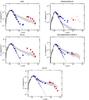 |
Fig. 2 SEDs of the five transitional disk candidates identified with Herschel. Blue dots represent the dereddened ancillary data from the literature from previous studies. The red diamonds are the clear detections with Herschel, and the red triangles the upper limits wherever no clear detection in the maps was found. The gray solid line is the median SED from the Lupus sample of the 29 non-transitional disks in the region, and the gray shaded area the first and fourth quartiles. See Table 7 for more information. The dashed lines are the photospheric NextGen models from Allard et al. (2012). |
3.3.5. SSTc2dJ160111.6-413730
SSTc2dJ160111.6-413730 has a very peculiar SED (see Fig. 3) with no excess at any wavelengths between optical and 160 μm, but substantial potential excesses at 250–500 μm associated with a clear point source in the images (see Fig. 4). The low 70 μm upper limit is nevertheless consistent with the sensitivity limit of the observations.
Previous claims of such extreme types of objects have been made in the context of the DUNES Herschel key program, who named these objects “cold disks” because of their extreme nature (Krivov et al. 2013). Other authors have suggested background galaxies as the possible explanation (Gáspár & Rieke 2014). This object did not fulfill our classification criteria as transitional disk candidate.
3.3.6. Sz65 and Sz66
Objects Sz65 and Sz66 form a binary system, with a separation of 6.4′′ (Lommen et al. 2010), unresolved by Herschel (see Fig. 4). We inspected their SEDs to select the main contributor. We deduce that the primary source is Sz65 by studying the contour diagram of the image. The contour lines were centered at the position of source Sz65. Their MIPS24 and MIPS70 fluxes support this association. Then we set the Herschel fluxes of Sz66 as upper limits in Table 6 and in Fig. 3.
4. Discussion
4.1. Detection statistics
From an initial sample of 217 known Class II sources with spectroscopic membership confirmation in the Lupus clouds, 123 objects fell in at least one of the fields observed by the HGBS. In particular, 92 and 98 were in the PACS and SPIRE Lupus III maps, respectively; 12 and 15 were found in Lupus I PACS and SPIRE mosaics; and 10 objects were observed in Lupus IV with both instruments. From these sources we detected 35 objects, 32 in PACS70, two in PACS100, and one in SPIRE. We then discarded one, 2MASSJ1608537, as we could not unequivocally assign its Herschel photometry to the target.
Compared with a similar study in Chamaeleon (Ribas et al. 2013), here we report a Herschel detection rate of ~28% of the previously known objects in the region, comparable with the percentage in that work (~30%). The small differences in the distances to the regions (~150 pc for Chamaeleon vs. ~200 pc to Lupus III) might account for the small difference in the detection rate. Further analysis of the detection statistics of known and new sources in these regions with the HGBS data will be presented by Benedittini et al. (in prep.).
4.2. Incidence of transitional disks in Lupus
We report the detection of five transitional disk candidates in the Lupus molecular clouds based on Herschel and previous data of all spectroscopically confirmed Class II members of the association. Two transitional disks were known from previous works (Sz91 and Sz111), but the other three are new to the literature.
The Spitzer study of the Lupus clouds found a global disk fraction of 50–60% (Ribas et al. 2014), compatible with a relatively young age for the region of 1–2 Myr (Comerón 2008). However, the total sample in Merín et al. (2008) included objects without spectroscopic membership confirmation so it could have a certain level of contamination from background galaxies and/or old dusty AGB stars (see Mortier et al. 2011, for a spectroscopic survey of Spitzer selected candidate members in Lupus). This work, however, uses an input target list where all objects have spectroscopic membership confirmation and is therefore not affected.
The observed fraction of transitional disks in Lupus based on our Herschel detected sample is ~15%, which is comparable to the fractions measured in other such young and nearby regions (Espaillat et al. 2014). This corrects a surprisingly low incidence of this type of objects from the Spitzer sample reported in Merín et al. (2008), where only two objects were identified as transitional out of a photometric sample of 139 Class II and III sources. This demonstrates how Herschel efficiently complements mid-infrared surveys for the specific study of transitional disks.
4.3. Brighter PACS-70 fluxes in transitional disks
Recent studies have reported brighter 70 μm fluxes in transitional disks as compared with the median SED of standard T Tauri stars in the same regions (Cieza et al. 2011; Ribas et al. 2013). To check whether this phenomenon is dependent on the conditions of certain molecular clouds, we compared the SEDs of the detected disks in Lupus with the median SED of T Tauri stars in the region. Figures 2 and 3 show the median SED normalized to the dereddened J-band flux for comparison, and Table 7 shows the fluxes of this median SED.
As shown in Fig. 2 most transitional disk candidates identified in Sect. 3.1 show the same phenomenon: the PACS fluxes are systematically above the median SED of the T Tauri stars. Therefore, the result has been confirmed around the isolated transitional disk T Cha (Cieza et al. 2011), in the Chamaeleon I cloud (Ribas et al. 2013), and in the Lupus molecular clouds (this work).
The interpretation of this phenomenon requires detailed SED modeling with radiative transfer disk models. However, the higher PACS fluxes compared with the median SED of the T Tauri stars suggests that the inner and outer disks of these objects follow different evolutionary paths by the time the inner gaps or holes are formed in the inner disks. Thus, the evolution of both inner and outer disk regions might not be dynamically decoupled.
4.4. SED population analysis
Merín et al. (2008) classified the YSO population in Lupus by studying the shape of their SEDs, and comparing the median SED of the CTTS from Taurus with their data. They grouped the objects into four categories, based on whether their slopes decay like a classical accreting optically thick disk around a low-mass star (T-Type), or if they present infrared excess clearly weaker (L-Type) or stronger (H-Type) than the median SED or where no excess is detected (E-Type). They also introduced a category that they called cold disks (LU-Type), which corresponds to our criteria for transitional disks. In their work, they made use of Spitzer and ground based photometry.
We did the same analysis for the 34 objects detected by Herschel, but now also taking into account the photometry we extracted. For simplification, we used a different nomenclature, grouping our objects into three categories that reveal their evolutionary state: higher infrared excess than the median values (H), indicating an early evolutionary stage; weaker (W), showing a more evolved stage; and transitional candidate (T). The results can be found in Table 5, where we also compare our classification to the aforementioned work by Merín et al. (2008). Another difference is that instead of using the Taurus median SED, we have used the Lupus value/values.
Apart from the transitional nature for the three new objects found in this work (~10%), we find that by adding the Herschel photometry to the SEDs we can update the type found in Merín et al. (2008) for another nine objects (~27%). The final population for our sample is then classified as follows: ~56% primordial disks (this groups T Tauri types and stronger infrared excesses), ~29% evolved disks, and ~15% transitional disk candidates. This compares well to the 67%, 26%, and 7% found for the same types of objects from the Spitzer-only study. Table 5 shows the Spitzer-only and Spitzer + Herschel classifications. The relative overall fractions have not changed substantially, except on the larger fraction of transitional disk candidates.
5. Conclusions
We have detected 34 objects in the Lupus cloud using Herschel and broadened the study of the YSOs in the association. Having confirmed that our Herschel data enable improved characterization of the outer regions of protoplanetary disks, we have identified additional transitional disks in our sample. The fraction of transitional disks detected in our study, comparable in size to Ribas et al. (2013), corrects the relatively low value from Spitzer detections. In addition, we find that all of these objects have 70 μm fluxes brighter than the median SED, showing perhaps another possible intrinsic property. Finally, we have carried out a population analysis by studying the SED shapes of the detections, and updated the morphological type of several sources. Further studies and modeling will give us more information on (about) these objects.
Online material
Class II objects detected by Herschel in the Lupus clouds.
Herschel photometry for the 34 YSOs detected in the maps.
Normalized flux densities of the median SED, lower SED (first quartile), and upper SED (fourth quartile) of the Class II objects in Lupus I, III, and IV.
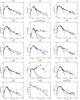 |
Fig. 3 SEDs of the 29 YSOs with Herschel detections that do not fulfill our transitional disk selection criteria. |
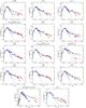 |
Fig. 3 continued. |
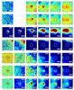 |
Fig. 4 Images of each of the 34 sources with at least one point source detected by Herschel, plus object 2MASSJ1608537, added for completeness. The images correspond to a box of 120′′ × 120′′ in size. Coordinates are given in Table 5. The color scale is defined with the root-mean square of the pixel values (as background level) and this number plus three times the standard deviation (as maximum level). North is up and east is left. A circle indicates the expected position of the target. The standard deviation computed around the sources is shown for each image (bottom right). |
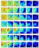 |
Fig. 4 continued. |
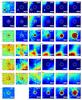 |
Fig. 4 continued. |
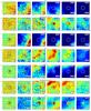 |
Fig. 4 continued. |
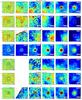 |
Fig. 4 continued. |
Acknowledgments
This work has been possible thanks to the ESAC Science Operations Division research funds with code EXPRO IPL-PSS/GP/gp/44.2014, plus support from the ESAC Space Science Faculty and of the Herschel Science Centre. We thank the referee for valuable comments which have helped to improve the paper. We also acknowledge Isabel Rebollido, Pablo Riviere-Marichalar, Bruno Altieri, Gabor Marton and the members of the Herschel Science Centre for discussions and extra checks on the Herschel/PACS photometry on large SPIRE/PACS parallel-mode maps of galactic fields. H. Bouy is funded by the Spanish Ramón y Cajal fellowship program number RYC-2009-04497. In the present paper we will be discussing observations performed with the ESA Herschel Space Observatory (Pilbratt et al. 2010), in particular employing Herschel’s large telescope and powerful science payload to do photometry using the PACS (Poglitsch et al. 2010) and SPIRE (Griffin et al. 2010) instruments. HCSS/HIPE is a joint development by the Herschel Science Ground Segment Consortium, consisting of ESA, the NASA Herschel Science Center, and the HIFI, PACS and SPIRE consortia. This research has made use of the SIMBAD database, operated at the CDS, Strasbourg, France. This work has made an extensive use of Topcat (TOPCAT http://www.star.bristol.ac.uk/~mbt/topcat/ and STILTS, Taylor 2005, 2006). This work makes use of data from the DENIS Survey. DENIS is the result of a joint effort involving human and financial contributions of several Institutes mostly located in Europe. It has been supported financially mainly by the French Institut National des Sciences de l’Univers, CNRS, and French Education Ministry, the European Southern Observatory, the State of Baden-Wuerttemberg, and the European Commission under networks of the SCIENCE and Human Capital and Mobility programs, the Landessternwarte, Heidelberg and Institut d’Astrophysique de Paris. This publication makes use of data products from the Wide-field Infrared Survey Explorer, which is a joint project of the University of California, Los Angeles, and the Jet Propulsion Laboratory/California Institute of Technology, funded by the National Aeronautics and Space Administration. This research used the facilities of the Canadian Astronomy Data Centre operated by the National Research Council of Canada with the support of the Canadian Space Agency. This publication makes use of data products from the Two Micron All Sky Survey, which is a joint project of the University of Massachusetts and the Infrared Processing and Analysis Center/California Institute of Technology, funded by the National Aeronautics and Space Administration and the National Science Foundation. This work is based in part on observations made with the Spitzer Space Telescope, which is operated by the Jet Propulsion Laboratory, California Institute of Technology under a contract with NASA.
References
- Allard, F., Homeier, D., & Freytag, B. 2012, IAU Symp. 282, eds. M. T. Richards, & I. Hubeny, 235 [Google Scholar]
- Allen, P. R., Luhman, K. L., Myers, P. C., et al. 2007, ApJ, 655, 1095 [NASA ADS] [CrossRef] [Google Scholar]
- André, P., Men’shchikov, A., Bontemps, S., et al. 2010, A&A, 518, L102 [NASA ADS] [CrossRef] [EDP Sciences] [Google Scholar]
- Calvet, N., D’Alessio, P., Watson, D. M., et al. 2005, ApJ, 630, L185 [NASA ADS] [CrossRef] [Google Scholar]
- Cieza, L. A., Schreiber, M. R., Romero, G. A., et al. 2010, ApJ, 712, 925 [NASA ADS] [CrossRef] [Google Scholar]
- Cieza, L. A., Olofsson, J., Harvey, P. M., et al. 2011, ApJ, 741, L25 [NASA ADS] [CrossRef] [Google Scholar]
- Comerón, F. 2008, The Lupus Clouds, ed. B. Reipurth, 295 [Google Scholar]
- Espaillat, C., Muzerolle, J., Najita, J., et al. 2014, Protostars and Planets VI, eds. H. Beuther, R. S. Klessen, C. P. Dullemond, & T. Henning (Tucson: University of Arizona Press), 497 [Google Scholar]
- Gáspár, A., & Rieke, G. H. 2014, ApJ, 784, 33 [NASA ADS] [CrossRef] [Google Scholar]
- Ghez, A. M., White, R. J., & Simon, M. 1997, ApJ, 490, 353 [NASA ADS] [CrossRef] [Google Scholar]
- Griffin, M. J., Abergel, A., Abreu, A., et al. 2010, A&A, 518, L3 [Google Scholar]
- Hughes, J., Hartigan, P., Krautter, J., & Kelemen, J. 1994, AJ, 108, 1071 [NASA ADS] [CrossRef] [Google Scholar]
- Krautter, J., Wichmann, R., Schmitt, J. H. M. M., et al. 1997, A&AS, 123, 329 [NASA ADS] [CrossRef] [EDP Sciences] [Google Scholar]
- Krivov, A. V., Eiroa, C., Löhne, T., et al. 2013, ApJ, 772, 32 [NASA ADS] [CrossRef] [Google Scholar]
- Lada, C., Luhman, K., Muench, A., et al. 2006, Spitzer Proposal, 30033 [Google Scholar]
- Lestrade, J.-F., Matthews, B. C., Sibthorpe, B., et al. 2012, A&A, 548, A86 [NASA ADS] [CrossRef] [EDP Sciences] [Google Scholar]
- Lommen, D. J. P., van Dishoeck, E. F., Wright, C. M., et al. 2010, A&A, 515, A77 [NASA ADS] [CrossRef] [EDP Sciences] [Google Scholar]
- Matrà, L., Merín, B., Alves de Oliveira, C., et al. 2012, A&A, 548, A111 [NASA ADS] [CrossRef] [EDP Sciences] [Google Scholar]
- Merín, B., Jørgensen, J., Spezzi, L., et al. 2008, ApJS, 177, 551 [NASA ADS] [CrossRef] [Google Scholar]
- Merín, B., Brown, J. M., Oliveira, I., et al. 2010, ApJ, 718, 1200 [NASA ADS] [CrossRef] [Google Scholar]
- Moreno-Corral, M. A., Chavarria-K., C., & de Lara, E. 1995, in Rev. Mex. Astron. Astrofis. Conf. Ser. 3, eds. M. Pena, & S. Kurtz, 121 [Google Scholar]
- Mortier, A., Oliveira, I., & van Dishoeck, E. F. 2011, MNRAS, 418, 1194 [NASA ADS] [CrossRef] [Google Scholar]
- Muzerolle, J., Allen, L. E., Megeath, S. T., Hernández, J., & Gutermuth, R. A. 2010, ApJ, 708, 1107 [NASA ADS] [CrossRef] [Google Scholar]
- Pilbratt, G. L., Riedinger, J. R., Passvogel, T., et al. 2010, A&A, 518, L1 [CrossRef] [EDP Sciences] [Google Scholar]
- Poglitsch, A., Waelkens, C., Geis, N., et al. 2010, A&A, 518, L2 [NASA ADS] [CrossRef] [EDP Sciences] [Google Scholar]
- Ribas, Á., Merín, B., Bouy, H., et al. 2013, A&A, 552, A115 [NASA ADS] [CrossRef] [EDP Sciences] [Google Scholar]
- Ribas, Á., Merín, B., Bouy, H., & Maud, L. T. 2014, A&A, 561, A54 [NASA ADS] [CrossRef] [EDP Sciences] [Google Scholar]
- Roussel, H. 2012, Astrophysics Source Code Library [http://ascl.net/1209.012] [Google Scholar]
- Rygl, K. L. J., Benedettini, M., Schisano, E., et al. 2013, A&A, 549, L1 [NASA ADS] [CrossRef] [EDP Sciences] [Google Scholar]
- Skrutskie, M. F., Cutri, R. M., Stiening, R., et al. 2006, AJ, 131, 1163 [NASA ADS] [CrossRef] [Google Scholar]
- Strom, S. E., Edwards, S., & Strom, K. M. 1989, in The Formation and Evolution of Planetary Systems, eds. H. A. Weaver, & L. Danly (Cambridge: Cambridge University Press), 91 [Google Scholar]
- Traficante, A., Fuller, G. A., Pineda, J. E., & Pezzuto, S. 2015, A&A, 574, A119 [NASA ADS] [CrossRef] [EDP Sciences] [Google Scholar]
- Tsukagoshi, T., Momose, M., Hashimoto, J., et al. 2014, ApJ, 783, 90 [NASA ADS] [CrossRef] [Google Scholar]
- Weingartner, J. C., & Draine, B. T. 2001, ApJ, 548, 296 [NASA ADS] [CrossRef] [Google Scholar]
- Werner, M. W., Roellig, T. L., Low, F. J., et al. 2004, ApJS, 154, 1 [Google Scholar]
All Tables
Aperture, inner, and outer radii used in the photometry extraction process for each band, with their corresponding aperture corrections.
Sensitivity limits for each Herschel band in parallel mode at 60′′/s, as stated in the PACS/SPIRE Parallel Mode Observers’ Manual.
Normalized flux densities of the median SED, lower SED (first quartile), and upper SED (fourth quartile) of the Class II objects in Lupus I, III, and IV.
All Figures
|
Fig. 1 Identification of transitional disk candidates applying the color criteria from Ribas et al. (2013) to the Lupus Herschel data. |
| In the text | |
|
Fig. 2 SEDs of the five transitional disk candidates identified with Herschel. Blue dots represent the dereddened ancillary data from the literature from previous studies. The red diamonds are the clear detections with Herschel, and the red triangles the upper limits wherever no clear detection in the maps was found. The gray solid line is the median SED from the Lupus sample of the 29 non-transitional disks in the region, and the gray shaded area the first and fourth quartiles. See Table 7 for more information. The dashed lines are the photospheric NextGen models from Allard et al. (2012). |
| In the text | |
|
Fig. 3 SEDs of the 29 YSOs with Herschel detections that do not fulfill our transitional disk selection criteria. |
| In the text | |
|
Fig. 3 continued. |
| In the text | |
|
Fig. 4 Images of each of the 34 sources with at least one point source detected by Herschel, plus object 2MASSJ1608537, added for completeness. The images correspond to a box of 120′′ × 120′′ in size. Coordinates are given in Table 5. The color scale is defined with the root-mean square of the pixel values (as background level) and this number plus three times the standard deviation (as maximum level). North is up and east is left. A circle indicates the expected position of the target. The standard deviation computed around the sources is shown for each image (bottom right). |
| In the text | |
|
Fig. 4 continued. |
| In the text | |
|
Fig. 4 continued. |
| In the text | |
|
Fig. 4 continued. |
| In the text | |
|
Fig. 4 continued. |
| In the text | |
Current usage metrics show cumulative count of Article Views (full-text article views including HTML views, PDF and ePub downloads, according to the available data) and Abstracts Views on Vision4Press platform.
Data correspond to usage on the plateform after 2015. The current usage metrics is available 48-96 hours after online publication and is updated daily on week days.
Initial download of the metrics may take a while.