| Issue |
A&A
Volume 577, May 2015
|
|
|---|---|---|
| Article Number | A109 | |
| Number of page(s) | 7 | |
| Section | Planets and planetary systems | |
| DOI | https://doi.org/10.1051/0004-6361/201526031 | |
| Published online | 12 May 2015 | |
No variations in transit times for Qatar-1 b⋆,⋆⋆
1
Centre for Astronomy, Faculty of Physics, Astronomy and Informatics,
Nicolaus Copernicus University,
Grudziadzka 5,
87-100
Torun,
Poland
e-mail:
This email address is being protected from spambots. You need JavaScript enabled to view it.
2
Instituto de Astrofísica de Andalucía (IAA-CSIC),
Glorieta de la Astronomía 3,
18008
Granada,
Spain
3
Michael Adrian Observatorium, Astronomie Stiftung Trebur, 65428
Trebur,
Germany
4
University of Applied Sciences, Technische Hochschule Mittelhessen, ,
61169
Friedberg,
Germany
5
Institute of Astronomy, Bulgarian Academy of
Sciences, 72 Tsarigradsko Chausse
Blvd., 1784
Sofia,
Bulgaria
6
Astrophysikalisches Institut und
Universitäts-Sternwarte, Schillergässchen 2–3, 07745
Jena,
Germany
7
European Space Agency, ESTEC, SRE-S, Keplerlaan 1,
2201 AZ
Noordwijk, The
Netherlands
8
Institute of Applied Physics, Abbe Center of Photonics,
Friedrich-Schiller-Universität Jena, Max-Wien-Platz 1, 07743
Jena,
Germany
Received: 5 March 2015
Accepted: 23 March 2015
Abstract
Aims. The transiting hot-Jupiter planet Qatar-1 b exhibits variations in transit times that could be perturbative. A hot Jupiter with a planetary companion on a nearby orbit would constitute an unprecedented planetary configuration, which is important for theories of the formation and evolution of planetary systems. We performed a photometric follow-up campaign to confirm or refute transit timing variations.
Methods. We extend the baseline of transit observations by acquiring 18 new transit light curves acquired with 0.6−2.0 m telescopes. These photometric time series, together with data available in the literature, were analyzed in a homogenous way to derive reliable transit parameters and their uncertainties.
Results. We show that the dataset of transit times is consistent with a linear ephemeris leaving no hint of any periodic variations with a range of 1 min. We find no compelling evidence of a close-in planetary companion to Qatar-1 b. This finding is in line with a paradigm that hot Jupiters are not components of compact multiplanetary systems. Based on dynamical simulations, we place tighter constraints on the mass of any fictitious nearby planet in the system. Furthermore, new transit light curves allowed us to redetermine system parameters with better precision than reported in previous studies. Our values generally agree with previous determinations.
Key words: planets and satellites: individual: Qatar 1b / stars: individual: Qatar 1
Partly based on (1) data collected with telescopes at the Rozhen National Astronomical Observatory and (2) observations obtained with telescopes of the University Observatory Jena, which is operated by the Astrophysical Institute of the Friedrich-Schiller-University.
Tables of light curve data are only available at the CDS via anonymous ftp to cdsarc.u-strasbg.fr (130.79.128.5) or via http://cdsarc.u-strasbg.fr/viz-bin/qcat?J/A+A/577/A109
© ESO, 2015
1. Introduction
The transiting planet Qatar-1 b (Alsubai et al. 2011) is the first planetary body discovered by the Qatar Exoplanet Survey (Alsubai et al. 2013). It is a typical hot Jupiter on a 1.42 d circular orbit. Alsubai et al. (2011) give a mass of 1.09 ± 0.08MJup (Jupiter’s mass), but new radial velocity (RV) measurements by Covino et al. (2013) show that the planet has a higher mass of 1.33 ± 0.05MJup. The published studies provide consistent determinations of a planetary radius that is greater by 16–18% than RJup (Jupiter’s radius). The planet produces transits that are nearly 1.5 h long and 2.3% deep in flux. The host star, GSC 4240-470 (V = 12.84 mag), is a metal-rich dwarf of spectral type K3. It exhibits a moderate chromospheric activity, which could be partly induced by the close-in planet (Covino et al. 2013). The RV observations throughout a transit show a signature of the Rositter-McLaughlin effect that is consistent with a sky-projected obliquity close to zero (Covino et al. 2013).
Details on instruments taking part in the campaign.
Details on individual light curves reported in this paper.
Redetermined system parameters, together with values from the literature.
More recently, von Essen et al. (2013) have found indications of long-term variations in transit timing residuals from a linear ephemeris. The periodicity of this signal is postulated to be close to 190 or 390 d with a peak-to-peak amplitude of about 2 min. These variations were interpreted as the result of the exchange of energy and angular momentum via gravitational interaction with an unseen, close-in planetary companion (Holman & Murray 2005; Agol et al. 2005). Such a planetary configuration would be unprecedented because hot Jupiters appear to be alone or accompanied by other planetary bodies on wide orbits (e.g., Steffen et al. 2012). On the other hand, studies of candidates for hot planets from a Kepler sample show that some fraction of these objects reveal periodic variations in transit timing that could be dynamically induced (Szabó et al. 2013). There may be only a small fraction of hot Jupiters that are part of compact multiple-planet systems. If such systems are confirmed, their properties will place constraints on planet formation and migration theories. In some circumstances, migration models based on tidal interactions between a giant planet and a circumstellar gas disk predict the presence of neighboring low-mass planets that are close to or trapped in interior or exterior mean-motion resonances (MMRs) with hot Jupiters (e.g., Podlewska & Szuszkiewicz 2009). Such resonant or near-resonant companions would induce orbital perturbations that produce detectable variations in transit times. The analysis of multiple-planet candidate systems shows that most planetary systems are not resonant, but the distribution of planet period ratios shows clumping just wide of low-order resonances, such as 2:1 or 3:2 (Fabrycky et al. 2014). The origin of this pattern is unclear. The questions of whether hot Jupiters are accompanied by planets on nearby orbits or not and what the fraction of such planetary configurations is still remain open.
In this context, Qatar-1 b with its preliminary detection of the transit time variation (TTV) signal could become a prototype of a new group of multiple-planet packed systems with hot Jupiters. As the system deserves further investigation, we organized an observing campaign to confirm or refute perturbations in the orbital motion of Qatar-1 b by the method of transit timing.
2. Observations
We acquired 18 new light curves for 16 transit events with six 0.6−2.0 m telescopes located across Europe (in Bulgaria, Poland, Germany, and Spain). The characteristics of individual instruments and detectors are given in Table 1. Two transits were observed simultaneously from two distinct sites. Most of the observations were performed in R filter, in which the instrumental setups were found to be the most effective. We also acquired light curves in white light, i.e. without any filter, to increase the signal-to-noise ratio and obtain more precise data for timing purposes. Telescopes were moderately defocused to observe the Qatar-1 star with exposure times between 10 s and 60 s, depending on mirror diameter, filter, and observing conditions. For a given light curve, the exposure time was kept fixed throughout a run. The timestamps were saved in coordinated universal time (UTC), provided by a GPS system or the network time protocol software. Details on individual runs are presented in Table 2.
Photometric time series were obtained with the differential aperture photometry applied to science images after bias and dark subtraction followed by flat-field correction with sky flats. The radius of the photometric aperture was optimized for each dataset to achieve the smallest scatter in the out-of-transit light curves. Magnitudes were determined against available comparison stars. Each light curve was detrended by fitting a parabola along with a trial transit model, then converted to fluxes and normalized to unity outside of the transit event. The timestamps were converted to barycentric Julian dates in barycentric dynamical time (BJDTDB, Eastman et al. 2010).
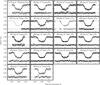 |
Fig. 1 New transit light curves acquired for Qatar-1 b, sorted by observation dates. The continuous lines show the best-fitting model, the residuals are plotted below each light curve. |
3. Results
3.1. System parameters
The Transit Analysis Package (TAP, Gazak et al. 2012) was used to model the set of 18 new transit light curves, supplemented with 31 complete or partial light curves available in the literature. Covino et al. (2013) provide five high-quality photometric time series acquired between May 2011 and September 2012 with the 1.82 m Asiago (Italy) and 1.23 m Calar Alto (Spain) telescopes. Von Essen et al. (2013) make 26 light curves available. They were obtained from March 2011 to August 2012 with the 1.2 m Oskar-Lühning telescope at Hamburg Observatory (Germany) and the 0.6 m Planet Transit Study Telescope at the Mallorca Observatory (Spain). The TAP code uses the Markov chain Monte Carlo (MCMC) method with the Metropolis-Hastings algorithm and a Gibbs sampler to find the best-fit transit model, based on the analytical approach of Mandel & Agol (2002). Since the photometric time series may be afflicted by time-correlated noise, the wavelet-based algorithm of Carter & Winn (2009) is employed to robustly estimate parameter uncertainties. A quadratic limb darkening (LD) law (Kopal 1950) is implemented to approximate the flux distribution across the stellar disk. The values of linear and quadratic LD coefficients, u1 and u2, respectively, were linearly interpolated from the tables of Claret & Bloemen (2011) using a dedicated tool of the EXOFAST package (Eastman et al. 2013). The stellar parameters, such as effective temperature Teff = 4910 ± 100 K, surface gravity log g = 4.55 ± 0.1 (in cgs units), and metallicity [ Fe/H ] = 0.2 ± 0.1, were taken from Covino et al. (2013). The efficient maximum of the energy distribution in white light was found to coincide with the R band, so R-band LD coefficients were adopted for white light curves.
In a final iteration of the fitting procedure, the orbital inclination ib, the semimajor-axis scaled by stellar radius ab/R∗, and the planetary to stellar radii ratio Rb/R∗ were linked for all light curves and fitted simultaneously. The midtransit times were determined independently for each epoch. The orbital period Pb was kept fixed at a value refined in Sect. 3.2. The LD coefficients were allowed to vary around the theoretical values under the Gaussian penalty of σ = 0.05 to account for uncertainties in stellar parameters and possible systematic errors of the theoretical predictions (e.g., Müller et al. 2013). The orbit of the planet was assumed to be circular (Covino et al. 2013). Although the individual light curves are detrended, the TAP code was allowed to take possible linear trends into account and include their uncertainties in the total error budget of the fit. We used ten MCMC chains, each containing 106 steps. The first 10% of the results were discarded from each chain to minimize the influence of the initial values of the parameters. The best-fitting parameters, determined as the median values of marginalized posteriori probability distributions, and 1 σ uncertainty estimates, defined by a range of 68.3% values of the distributions, are given in Table 3. The new light curves are plotted in Fig. 1, together with the transit model and residuals.
The parameters derived from the transit model, combined with literature quantities determined from spectroscopic data, allowed us to redetermine the stellar mass M∗, luminosity L∗, and system age. The mean stellar density ρ∗ was calculated from transit parameters, independent of theoretical stellar models, using the formula 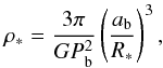 (1)where G is the universal gravitational constant. Then, the host star was placed at a modified Hertzsprung-Russel diagram (Fig. 2) displaying the
  versus Teff plane, together with parsec isochrones in version 1.2S (Bressan et al. 2012). The stellar parameters and their uncertainties were derived by interpolating the sets of isochrones with [ Fe/H ] ranging from 0.1 to 0.3.
The parameters ib and Rb/R∗ were checked for long timescale trends or periodic variability (ab/R∗ was not considered because it is correlated with ib). The fitting procedure was repeated for a subset of 37 complete light curves, with ib and Rb/R∗ allowed to be determined independently for each dataset. The parameter ab/R∗ was allowed to vary around a best-fit value under the Gaussian penalty, as given in Table 3. Individual determinations are plotted in Fig. 3. A model assuming a constant ib has a reduced chi-squared  of 1.15 and a p-value of 0.25. The parameter Rb/R∗ is also constant with
  , which corresponds to a p-value of 0.15. For both parameters, there is no reason to reject a null hypothesis assuming constancy. In addition, both parameters were searched for periodic variations with the Lomb-Scargle algorithm (Lomb 1976; Scargle 1982), and no significant signal was found. The lack of any variations justifies linking these parameters in the final model.
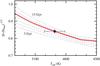 |
Fig. 2 Modified Hertzsprung-Russel diagram with Qatar-1 marked as a central dot. The PARSEC isochrones of [ Fe/H ] = 0.20 and ages between 3 and 13 Gyr with a step of 2 Gyr are sketched with dashed lines. The best-fitting isochrone is drawn with a continuous line. |
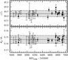 |
Fig. 3 Distribution of ib and Rb/R∗ in a function of time for a trial fit, in which both parameters were allowed to vary for individual complete transit light curves. Open and filled symbols represent the literature and our new datasets, respectively. Continuous lines denote weighted mean values. Grayed areas between dashed lines show uncertainties at the confidence level of 95.5%, i.e. 2σ, where σ is the weighted standard deviation. |
3.2. Transit timing
New midtransit times, together with redetermined values from the literature data, allowed us to refine the transit ephemeris. As a result of a least-square linear fit, in which timing uncertainties were taken as weights, we derived  (2)and the midtransit time at cycle zero
  (3)The value of was found to be equal to 1.07, clearly showing that there is no hint of any deviation from the constant orbital period. The procedure was repeated for a limited sample of 17 midtransit times with uncertainties smaller than 40 s, hence the most reliable. Again, the linear ephemeris was found to reproduce observed transits perfectly with
  . This shows that any possible TTV signal is not masked by a scatter of data points of lower quality, hence lower timing precision. Individual transit times and residuals are collected in Table 4, and residuals from the ephemeris are plotted in Fig. 4.
The Lomb-Scargle periodogram (Fig. 5) reveals no significant power at periods of 187 ± 17 and 386 ± 54 d, reported by von Essen et al. (2013). A bootstrap resampling method, based on 105 trials of the randomly permuted timing residuals at the original observing epochs, was used to determine a false alarm probability (FAP) of 28% for the strongest peak.
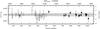 |
Fig. 4 Residuals of transit times from the refined linear ephemeris. Open symbols indicate the literature data. Filled dots denote new transits reported in this paper. The midtransit time at epoch 181 (2011 Aug. 01 = BJD 2 455 775.4), marked with a half-filled symbol, is determined using a light curve from von Essen et al. (2013) and a light curve reported in this paper. The grayed area between dashed lines shows the propagation of uncertainties of the ephemeris at a 95.5% confidence level. |
New and redetermined mid-transit times.
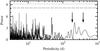 |
Fig. 5 Lomb-Scargle periodogram for timing residuals plotted in Fig. 4. Dashed and dotted horizontal lines show the 5% and 1% FAP levels, respectively. Arrows indicate positions of the TTV signals claimed by von Essen et al. (2013). |
3.3. Constraints on an additional planet
The TTV method is particularly sensitive to perturbers close to MMRs. The non-detection of periodic variations in transit timing allows such planetary configurations to be ruled out. In the remaining configurations, planetary companions may be detected more easily in the domain of precise Doppler measurements. Combining these two methods places constraints on an upper mass of any hypothetical second planet in the system as a function of its semi-major axis.
We followed the method that we applied to WASP-3 and WASP-1 systems (Maciejewski et al. 2013, 2014). The Bulirsch-Stoer integrator, implemented in the Mercury 6 code (Chambers 1999), was used to predict deviations from a Keplerian motion of Qatar-1 b caused by a fictitious perturbing planet. The system was assumed to be coplanar, with both orbits initially circular. The mass of the perturber was set at 0.5, 1, 5, 10, 50, 100, and 500 MEarth (Earth masses), and the initial semi-major axis varied between 0.023 and 0.107 AU (corresponding to the orbital period ratio between 1 and 10) with a step of 2 × 10⁻⁶ AU. Only configurations with an outer perturber were considered because of the short orbital period of Qatar-1 b. The initial orbital longitude of the transiting planet was set to a value calculated for cycle zero, and the initial longitude of the fictitious perturber was shifted by 180°. The calculations covered a time span of 1500 days in which transits of Qatar-1 b were observed. The residuals from a linear ephemeris for synthetic datasets were compared with the observed root-mean square (rms) of transit timing, and a TTV upper mass of a fictitious planet was calculated.
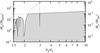 |
Fig. 6 Upper mass limit for a fictitious outer planet in the planetary system around Qatar-1, based on timing and RV datasets, as a function of the orbital period of that planet, Pp. Configurations that are below the detection threshold of both techniques are placed in the grayed space of parameters, bounded by a continuous line. The dotted and dashed lines show detection limits for timing and RV techniques, respectively. Configurations with Pp/Pb< 1.5 were found to be unstable on a short timescale of the simulations. |
Reanalysis of the RV dataset from Covino et al. (2013), performed with the Systemic 2.16 (Meschiari et al. 2009), gives a circular single-planet orbit with rmsRV = 11.1 m s-1. The RV measurements were acquired with the High Accuracy Radial velocity Planet Searcher-North (HARPS-N) spectrograph installed at the 3.58 m Telescopio Nazionale Galileo (TNG) on La Palma (Spain). The RV uncertainties are between 4.4 and 20 m s-1. The dataset from Alsubai et al. (2011), acquired with the Tillinghast Reflector Echelle Spectrograph (TRES) coupled with the 1.5-m telescope at the Fred L. Whipple Observatory (USA), was omitted because of the much lower precision of the RV measurements (22−61 m s-1). The value of rmsRV was transformed into the RV mass limit of the hypothetical second planet on a circular orbit as a function of its semi-major axis.
Finally, the TTV and RV criteria were combined to find planetary configurations with a hypothetical second planet below the detection threshold. Results are illustrated in Fig. 6. The TTV technique is more sensitive for configurations within the 2:1 resonance. We can eliminate perturbers with masses between 10 and 20 MEarth out of MMRs and probe for a sub-Earth mass regime in 2:1 and 5:3 MMRs. For orbital periods longer than about 2.2 Pb, the Doppler dataset provides tighter constraints except for 3:1 MMR, in which a perturber with a mass down to about 3 MEarth can be eliminated thanks to the TTV method.
4. Concluding discussion
Despite the conservative approach, our light curve modeling provides system parameters with the smallest uncertainties published so far. This is the result of the homogenous analysis of the rich set of 18 new and 31 earlier light curves. The orbital inclination  agrees perfectly with the value of
  reported by von Essen et al. (2013), and differs by 1.1 and 1.4σ from results of Covino et al. (2013) and Alsubai et al. (2011), respectively. The scaled semi-major axis
 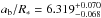 is between 6.25 ± 0.10 and 6.42 ± 0.10 as found by Covino et al. (2013) and von Essen et al. (2013), respectively. The planet-to-star radii ratio
  is consistent with 0.1453 ± 0.0016 as derived by Alsubai et al. (2011), and it differs by 1.5σ and 3.5σ from values reported by von Essen et al. (2013) and Covino et al. (2013), respectively. Planetary physical properties derived in this study confirm results of Covino et al. (2013), and deviate slightly from values reported by Alsubai et al. (2011) because the planetary mass was underestimated in that study. Stellar parameters were found to agree with values determined in previous studies. The system’s age is ≈10 Gyr with the lower uncertainty of ≈6 Gyr and the upper one limited by the age of the Universe. The host star is in the middle of its lifetime on the main sequence, which is estimated to be ≈18 Gy for a 0.8 M⊙ star.
Spectral observations of the Ca II H and K lines show that the host star exhibits a moderate chromospheric activity with  (Covino et al. 2013). However, we find no statistically significant variation in the planet-to-star radii ratio that could be caused by the evolving distribution of dark spots or bright faculae outside the projected path of the planet on the stellar disk (e.g., Czesla et al. 2009). We also identified no features in the transit light curves that could be attributed to starspot occultations by the planetary disk.
Transit timing observations clearly show that the orbital motion of Qatar-1 b is not perturbed by any body that could produce periodic deviations with a range greater than one minute. We find no evidence to confirm the TTV signal with the periodicity and amplitude reported by von Essen et al. (2013). Combining the transit timing and RV datasets, we can rule out three proposed scenarios with perturbers in 2:1, 5:2, and 3:1 resonances even for circular orbits. (In general, eccentric orbits make perturbations more pronounced.) The lack of the TTV signal also makes a proposed massive perturber on a wide orbit unlikely. We note, however, that further RV measurements, acquired in the course of a few hundred days, would unequivocally reject this scenario.
We conclude that Qatar-1 b has no detectable planetary companions on nearby orbits. This finding is in line with results based on a sample of hot Jupiters observed with the space-borne facilities or ground-based telescopes. Since the formation of hot
Jupiters is not yet fully understood (e.g., Steffen et al. 2012), the loneliness of Qatar-1 b speaks in favor of inward migration theories of massive outer planets through the planet-planet scattering caused by mutual dynamical perturbations (Weidenschilling & Marzari 1996; Rasio & Ford 1996).
Acknowledgments
M.K. thanks the German national science foundation, Deutsche Forschungsgemeinschaft (DFG), for financial support in projects NE515/34-1.34-2 and R.E. 882/12-2. S.R. is currently a Research Fellow at ESA/ESTEC. S.R. would like to thank the DFG for support in the Priority Program SPP 1385 on the “First Ten Million Years of the Solar System” in projects NE 515/33-1 and -2. R.E. thanks the Abbe-School of Photonics for support. AP acknowledges support from the DFG in SFB TR7 project C2. J.G.S. thanks DFG in SFB TR7 project B9 for support. We would like to acknowledge financial support from the Thuringian government (B 515-07010) for the STK CCD camera used in this project.
References
- Agol, E., Steffen, J., Sari, R., & Clarkson, W. 2005, MNRAS, 359, 567 [NASA ADS] [CrossRef] [Google Scholar]
- Alsubai, K. A., Parley, N. R., Bramich, D. M., et al. 2011, MNRAS, 417, 709 [NASA ADS] [CrossRef] [Google Scholar]
- Alsubai, K. A., Parley, N. R., Bramich, D. M., et al. 2013, Acta Astron., 63, 465 [NASA ADS] [Google Scholar]
- Bressan, A., Marigo, P., Girardi, L., et al. 2012, MNRAS, 427, 127 [NASA ADS] [CrossRef] [Google Scholar]
- Carter, J. A., & Winn, J. N. 2009, ApJ, 704, 51 [NASA ADS] [CrossRef] [Google Scholar]
- Chambers, J. E. 1999, MNRAS, 304, 793 [NASA ADS] [CrossRef] [MathSciNet] [Google Scholar]
- Claret, A., & Bloemen, S. 2011, A&A, 529, A75 [NASA ADS] [CrossRef] [EDP Sciences] [Google Scholar]
- Covino, E., Esposito, M., Barbieri, M., et al. 2013, A&A, 554, A28 [NASA ADS] [CrossRef] [EDP Sciences] [Google Scholar]
- Czesla, S., Huber, K. F., Wolter, U., Schröter, S., & Schmitt, J. H. M. M. 2009, A&A, 505, 1277 [NASA ADS] [CrossRef] [EDP Sciences] [Google Scholar]
- Eastman, J., Siverd, R., & Gaudi, B. S. 2010, PASP, 122, 935 [NASA ADS] [CrossRef] [Google Scholar]
- Eastman, J., Gaudi, B. S., & Agol, E. 2013, PASP, 125, 83 [NASA ADS] [CrossRef] [Google Scholar]
- Fabrycky, D. C., Lissauer, J. J., Ragozzine, D., et al. 2014, ApJ, 790, 146 [NASA ADS] [CrossRef] [Google Scholar]
- Fulton, B. J., Shporer, A., Winn, J. N., et al. 2011, AJ, 142, 84 [NASA ADS] [CrossRef] [Google Scholar]
- Gazak, J. Z., Johnson, J. A., Tonry, J., et al. 2012, Adv. Astron., 2012, 30 [Google Scholar]
- Holman, M. J., & Murray, N. W. 2005, Science, 307, 1288 [NASA ADS] [CrossRef] [PubMed] [Google Scholar]
- Kopal, Z. 1950, Harvard College Observatory Circular, 454, 1 [Google Scholar]
- Lomb, N. R. 1976, Ap&SS, 39, 447 [NASA ADS] [CrossRef] [Google Scholar]
- Maciejewski, G., Niedzielski, A., Wolszczan, A., et al. 2013, AJ, 146, 147 [NASA ADS] [CrossRef] [Google Scholar]
- Maciejewski, G., Ohlert, J., Dimitrov, D., et al. 2014, Acta Astron., 64, 27 [NASA ADS] [Google Scholar]
- Mandel, K., & Agol, E. 2002, ApJ, 580, L171 [NASA ADS] [CrossRef] [Google Scholar]
- Meschiari, S., Wolf, A. S., Rivera, E., et al. 2009, PASP, 121, 1016 [NASA ADS] [CrossRef] [Google Scholar]
- Mugrauer, M., & Berthold, T. 2010, Astron. Nachr., 331, 449 [Google Scholar]
- Müller, H. M., Huber, K. F., Czesla, S., Wolter, U., & Schmitt, J. H. M. M. 2013, A&A, 560, A112 [NASA ADS] [CrossRef] [EDP Sciences] [Google Scholar]
- Podlewska, E., & Szuszkiewicz, E. 2009, MNRAS, 397, 1995 [NASA ADS] [CrossRef] [Google Scholar]
- Rasio, F. A., & Ford, E. B. 1996, Science, 274, 954 [NASA ADS] [CrossRef] [PubMed] [Google Scholar]
- Scargle, J. D. 1982, ApJ, 263, 835 [NASA ADS] [CrossRef] [Google Scholar]
- Steffen, J. H., Ragozzine, D., Fabrycky, D. C., et al. 2012, Proc. Nat. Acad. Sci., 109, 7982 [NASA ADS] [CrossRef] [Google Scholar]
- Szabó, R., Szabó, G. M., Dálya, G., et al. 2013, A&A, 553, A17 [NASA ADS] [CrossRef] [EDP Sciences] [Google Scholar]
- von Essen, C., Schröter, S., Agol, E., & Schmitt, J. H. M. M. 2013, A&A, 555, A92 [NASA ADS] [CrossRef] [EDP Sciences] [Google Scholar]
- Weidenschilling, S. J., & Marzari, F. 1996, Nature, 384, 619 [NASA ADS] [CrossRef] [PubMed] [Google Scholar]
All Tables
All Figures
|
Fig. 1 New transit light curves acquired for Qatar-1 b, sorted by observation dates. The continuous lines show the best-fitting model, the residuals are plotted below each light curve. |
| In the text | |
|
Fig. 2 Modified Hertzsprung-Russel diagram with Qatar-1 marked as a central dot. The PARSEC isochrones of [ Fe/H ] = 0.20 and ages between 3 and 13 Gyr with a step of 2 Gyr are sketched with dashed lines. The best-fitting isochrone is drawn with a continuous line. |
| In the text | |
|
Fig. 3 Distribution of ib and Rb/R∗ in a function of time for a trial fit, in which both parameters were allowed to vary for individual complete transit light curves. Open and filled symbols represent the literature and our new datasets, respectively. Continuous lines denote weighted mean values. Grayed areas between dashed lines show uncertainties at the confidence level of 95.5%, i.e. 2σ, where σ is the weighted standard deviation. |
| In the text | |
|
Fig. 4 Residuals of transit times from the refined linear ephemeris. Open symbols indicate the literature data. Filled dots denote new transits reported in this paper. The midtransit time at epoch 181 (2011 Aug. 01 = BJD 2 455 775.4), marked with a half-filled symbol, is determined using a light curve from von Essen et al. (2013) and a light curve reported in this paper. The grayed area between dashed lines shows the propagation of uncertainties of the ephemeris at a 95.5% confidence level. |
| In the text | |
|
Fig. 5 Lomb-Scargle periodogram for timing residuals plotted in Fig. 4. Dashed and dotted horizontal lines show the 5% and 1% FAP levels, respectively. Arrows indicate positions of the TTV signals claimed by von Essen et al. (2013). |
| In the text | |
|
Fig. 6 Upper mass limit for a fictitious outer planet in the planetary system around Qatar-1, based on timing and RV datasets, as a function of the orbital period of that planet, Pp. Configurations that are below the detection threshold of both techniques are placed in the grayed space of parameters, bounded by a continuous line. The dotted and dashed lines show detection limits for timing and RV techniques, respectively. Configurations with Pp/Pb< 1.5 were found to be unstable on a short timescale of the simulations. |
| In the text | |
Current usage metrics show cumulative count of Article Views (full-text article views including HTML views, PDF and ePub downloads, according to the available data) and Abstracts Views on Vision4Press platform.
Data correspond to usage on the plateform after 2015. The current usage metrics is available 48-96 hours after online publication and is updated daily on week days.
Initial download of the metrics may take a while.