| Issue |
A&A
Volume 577, May 2015
|
|
|---|---|---|
| Article Number | A61 | |
| Number of page(s) | 7 | |
| Section | The Sun | |
| DOI | https://doi.org/10.1051/0004-6361/201525960 | |
| Published online | 05 May 2015 | |
The low energy magnetic spectrometer on Ulysses and ACE response to near relativistic protons
1 Laboratório de Instrumentação e Física experimental de Partículas (LIP), Avenida Elias Garcia, 1000-149 Lisboa, Portugal
2 CICGE, Faculdade de Ciências da Universidade do Porto, Observatório Astronómico Professor Manuel de Barros, 4430-146 Vila Nova de Gaia, Portugal
e-mail: This email address is being protected from spambots. You need JavaScript enabled to view it.
3 Center for Solar-Terrestrial Research, New Jersey Institute of Technology, Newark, New Jersey 07102, USA
4 Fundamental Technologies, LLC, 2411 Ponderosa Dr. Lawrence, KS 66046, USA
Received: 24 February 2015
Accepted: 25 March 2015
Abstract
Aims. We show that the Heliosphere Instrument for Spectra Composition and Anisotropy at Low Energies (HISCALE) on board the Ulysses spacecraft and the Electron Proton Alpha Monitor (EPAM) on board the Advance Composition Explorer (ACE) spacecraft can be used to measure properties for ion populations with kinetic energies in excess of 1 GeV. This previously unexplored source of information is valuable for understanding the origin of near relativistic ions of solar origin.
Methods. We model the instrumental response from the low energy magnetic spectrometers from EPAM and HISCALE using a Monte Carlo approach implemented in the Geant4 toolkit to determine the response of different energy channels to energies up to 5 GeV. We compare model results with EPAM observations for 2012 May 17 ground level solar cosmic ray event, including directional fluxes.
Results. For the 2012 May event, all the ion channels in EPAM show an onset more than one hour before ions with the highest nominal energy range (1.8 to 4.8 MeV) were expected to arrive. We show from Monte Carlo simulations that the timing at different channels, the ratio between counts at the different channels, and the directional fluxes within a given channel, are consistent with and can be explained by the arrival of particles with energies from 35 MeV to more than 1 GeV. Onset times for the EPAM penetrating protons are consistent with the rise seen in neutron monitor data, implying that EPAM and ground neutron monitors are seeing overlapping energy ranges and that both are consistent with GeV ions being released from the Sun at 10:38 UT.
Key words: Sun: activity / Sun: corona / Sun: particle emission
© ESO, 2015
1. Introduction
The Heliospheric Ion Spectra and Composition Analysis at Low Energies (HISCALE) experiment (Lanzerotti et al. 1992) on board the Ulysses spacecraft and the Electron Proton Alpha Monitor (EPAM) experiment (Gold et al. 1998) on board the Advanced Composition Explorer (ACE) spacecraft are nearly identical suites of instruments designed to observe the energy spectra of electrons and protons with energies above 30 keV. For both sets of instruments, besides the field of view response, which for protons is limited to energies below 5 MeV, there is an “out of nominal passband” response, due to high energy particles penetrating through the instrument frame and giving “spurious” counts. By comparing the background seen at HISCALE with rates from the Charged Particle Measurement Experiment (CPME) on the Interplanetary Monitoring Platform (IMP-8) spacecraft Patterson & Armstrong (2001) show that the background rates on all energy channels in HISCALE are mostly due to penetrating Galactic cosmic rays (GCR) of energy in the range measured by CPME P11 energy channel (145 to 440 MeV per nucleon) and greater. This spurious component has essentially been viewed as a contaminant, and its subtraction from ion data was required to determine the steady-state, event-excluded ion spectra in the heliosphere (Patterson & Armstrong 2003).
If penetrating particles show a quantitatively meaningful signature at the relatively low levels of GCRs fluxes, then EPAM and HISCALE might be able to detect enhancements in their count rates during solar energetic particle events extending into hundreds of MeVs, in particular those related to ground level enhancements (GLEs). For that purpose, in this paper we first characterize the instrument out of nominal passband response using Monte Carlo techniques and a model of the EPAM and HISCALE particle telescopes, and then we analyze the GLE of solar cycle 24, on 2012 May 17, to show that EPAM’s response is consistent with the detection of protons of solar origin with energies about 1 GeV. This kind of information generally has only been available from ground instruments like neutron radiation monitors.
2. The LEMS120 telescope
The EPAM and HISCALE consist of five telescope apertures, mounted with fixed angles to the spacecraft rotation axis. Both suites of instruments include two low energy magnetic spectrometers (LEMS30 and LEMS120), two low energy foil spectrometers (LEFS150 and LEFS60), and a composition aperture (CA60) detector; where the number after the telescope name indicates the inclination of the telescope axis with respect to the spacecraft spin axis. The five separate detector systems are contained within two structures, known as LAN2A and LAN2B.
We focus on opening angles and spin-axis orientations of the LAN2A assembly, which are illustrated in the schematic in Fig. 1. In subsequent sections, we follow the notation from Fig. 1, using M’ and F’ to indicate the detector pair in LAN2A. This detector pair consists of two equal 200 μm thick totally depleted circular silicon surface barrier detectors with 5652 μm radius. LEMS30 and LEFS150 form a similar assembly, but the behavior from LAN2B became erratic on EPAM following the Halloween ion events in 2003 (Haggerty et al. 2006) so we do not use those data. The LEMS120 telescope contains magnets designed to deflect electrons with energies higher than 300 keV away from the detector M’; ions are not deflected and are thus able to hit the M’ detector. LEMS120 is thus essentially an ion detector with eight nominal energy channels designated from P’1 to P’8. We concentrate on only three of those channels P’2 (68−115 keV nominal energy range), P’3 (115−195 keV), and P’8 (1.9−4.8 MeV).
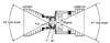 |
Fig. 1 LAN2A assembly of the EPAM instrument, formed by the LEMS120 and LEFS60 telescopes. |
Relevant EPAM LEMS120 discriminator levels.
The LEMS/LEFS systems provide pulse-height-analyzed single-detector measurements with active anticoincidence where energies deposited in the active silicon volume are assigned to a given channel according to discriminator levels set by the electronics. A charge-sensitive preamplifier produces output proportional to the energy absorbed plus a given amount of preamplifier noise. The discriminator response function DR(E) is approximately given by a complementary error function, 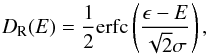 where ϵ is the discriminator level, E the deposited energy, and σ the preamplifier noise level. We refer to the discriminator levels for the M’ detector as M’0 to M’7, ordered from low to high. Documentation available for HISCALE refers a value of 10 keV for the noise levels and this value is accurate enough for our purposes. The discriminator levels for LEMS120 on EPAM and associated noise are reported in Table 1; we determined more accurate values for the noise in M’0 and M’1 based on preflight calibration. Values for HISCALE discriminator levels differ only slightly.
The nominal energy range for the LEMS120 channels does not correspond to the actual energy deposited in the active silicon volume. Before reaching the silicon, particles need to cross a 184 nm thick aluminum contact. The energy lost in that contact is accounted for when defining the nominal energy range and as such the discriminator levels set by the electronics correspond to a deposition of energy in the detector slightly lower than the nominal energy values. The deposited energy value is important for the simulations we discuss later, rather than the nominal energy range.
The anticoincidence implemented by the electronics is of paramount importance in understanding the counts given by EPAM and HISCALE; for a discussion applied to the electron channels see Haggerty & Roelof (2006). The anticoincidence defines the energy channel to which a given particle is assigned. As an example, a particle gives a count on P’1 if its energy deposited is enough to trigger M’0 but not M’1. This anticoincidence also includes the response from the F’ detector sitting in front of M’. A proton incident on M’ in a near-perpendicular direction with energy above 4.8 MeV does not deposit the totality of its energy when traveling 200 μ of silicon so that it will give a nearly simultaneous response in F’; this anticoincidence with F’ is used to reject field of view ions with energies higher than 4.8 MeV.
2.1. Response to penetrating ions
From the LAN2A engineering drawings, we know that the lowest thickness of the stainless steel enveloping the detector chamber and the adjacent magnet chamber is about 0.09 inches, being substantially larger in the projections supporting the magnet. This means that protons of energies lower than about 35 MeV can only hit the detector if they are “field of view protons”. Substantially higher energy protons should be able to cross some of the thicker portions of the shielding, and even the material providing support and connecting LEMS120 to the rest of the instrument and to the spacecraft body.
The simplest case is to consider what happens at energies substantially higher than the cutoff given by the frame enveloping the detectors. When considering protons of sufficiently high energy, as will be that case for those in the GeV range, one can mostly ignore the energy loss in the iron frame and support structure and address only what will happen in the silicon; we take this approach here. We did the simulations of proton interaction with silicon using the Geant4 toolkit (Geant4 Collaboration et al. 2003). Although the average energy loss can be computed reasonably well using the Bethe-Bloch equation, a Monte-Carlo approach as that given by Geant4 allows us to look at the shape of the distribution of deposited energies.
We show in Fig. 2 the distribution of deposited energies for primaries of 5.3 GeV and 384 MeV for normal incidence on a 200 μm thick silicon waffle; the gray band marks the energy range corresponding to P’2. The shape of the responses illustrated in Fig. 2 shows a very prompt rise with increasing deposited energy followed by a long a tail. Channels P’2 and P’3 respond to high energy protons, overlapping substantially in their response to hundred MeV to GeV incident protons, while P’8 is essentially insensitive to that energy range.
Of course, for normal incidence, penetrating protons of large energy would hit both M’ and F’ and thus would be rejected by the active anticoincidence mechanism implemented in LAN2A. As such, to be counted, high energy ions will need to reach the detector at oblique angles, thus traveling substantially more than for normal incidence. Since the deposited energy is roughly proportionally to the silicon distance traveled, the likelihood of being counted in a given channel will strongly depend on the direction that the proton comes from. We have included this effect in the simulations and discuss it next when presenting the 2012 May 17 event.
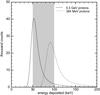 |
Fig. 2 Results from Monte Carlo simulations showing number of particles versus deposited energy for two incident proton energies. A million protons were simulated at each energy, propagating parallel to the detector normal and impacting the center of the detector; the gray band marks the energy range corresponding to P’2. |
3. Modeling the response for 2012 May 17
To illustrate LEMS120 response, including effects of directivity, we consider a very strongly anisotropic case, assuming that all particles are aligned with the magnetic field direction. This is close to the situation expected at the onset of an event of solar origin. We chose the direction the interplanetary magnetic field had relative to EPAM on 2014 May 17 at 02:00 UT; the results would have changed change very little if we had taken the magnetic field direction an hour before or later. We then simulated the rotation of the spacecraft and divided the spin period into eight identical intervals (sectors), mimicking the way data are gathered for LEMS120. We then simulated the instrumental response to protons of energies from 50 MeV to 5 GeV released uniformly in time; the same number of protons were modeled at each energy.
The simulation details very closely follow the procedure that is used to determine geometrical factors for particle telescopes. We generate proton coordinates randomly following a distribution uniform on the surface of a sphere. The dimensions of the sphere chosen were big enough to encompass both F’ and M’. Each test proton was then followed assuming they were initially propagating along a linear trajectory following the interplanetary magnetic field direction. We did simulations of proton interaction with silicon using the Geant4 toolkit. We then computed the deposited energy for each particle, and we attributed a channel to the particle using the values for the discriminator levels and noise given in Table 1; we included the effects of anticoincidence with F’. The results from the simulation allow the computation of a geometrical factor. To do so, we merely take the number of “test particles” that are assigned to the channel, on the basis of deposited energy, and divide that by the number of test particles that were “launched”, multiply by the area of the sphere they were launched from and finally multiply by 2 (since half of the launched particles would move outward from the sphere).
The results of the Monte Carlo simulations are shown in Fig. 3. While P’8 has a response to incident proton energies dropping sharply with increasing energy, with only residual sensitivity below 100 MeV, channels P’2 and P’3 show increased response at much higher energies. One of the important features in Fig. 3 is that P’2 response exceeds P’3 only for energies higher than ~1 GeV. Penetrating protons with primary energies sufficiently close to the cutoff provided by the instrument frame have a much wider range of directions available for positive detection since they might end up with energies low enough to enable full deposition in M’. This is a considerably more complex problem, since the geometry of the full assembly, including part of the spacecraft, needs to be considered. We do not pursue this further, although we note that 35 to 100 MeV protons should be very important for defining the P’8 response.
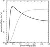 |
Fig. 3 Results from Monte Carlo simulations of protons hitting M’, showing the relative response, under the form of geometrical factors, of channels P’2 (thin full line), P’3 (thick full line), and P’8 (dashed line). |
We did not try to compensate for the question of instrument degradation with time, which can be a serious problem for particle telescopes based on solid state detectors (Wüest et al. 2007). Irradiation by 1012 to 1013 protons per centimeter square already cause damage to silicon detectors, and there is significant degradation after fluences of 1014 to 1015 protons per centimeter square: the detector efficiency may drop by a factor of 2 (Peltola 2014), and the noise levels may increase in such a way that the lowest channels discriminators become unusable. Total fluence in LEMS120 on EPAM since the mission start is about 1012, so the level of degradation should be relatively minor. We note nonetheless that, as discussed in Haggerty et al. (2006), the noise levels in P’1 on EPAM are indeed rather high and the counts often show a considerable number of spikes; we avoid using P’1 in the analysis follows.
4. EPAM observations of the 2012 May 17 event
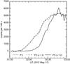 |
Fig. 4 Comparison of the counts from the LEMS120 P’2, P’3, and P’8 counts for 144 s integrations. Counts from P’3 and P’8 have been scaled so that the peak counts for all channels are at equivalent levels. |
A very thorough paper describing neutron monitor observations for the 2012 May 17 GLE is presented in Mishev et al. (2014) and we use results from that work extensively. In particular, Mishev et al. (2014) provide rigidity spectra for several periods during the event. We use the earliest time interval provided (from 02:00 to 02:10 UT) since at that time the pitch angle distribution should show the strongest anisotropy. For particles propagating close to the magnetic field direction we can then use the relative response of channel P’2 given in Fig. 3 to infer the expected count rates for that particular channel. We choose P’2 since it only shows a significant response for protons above 500 MeV, so that it is less affected by energy loss in the detector frame, something that we have not modeled. Neutron monitor data and the geometrical factor obtained from the model response of P’2 suggest that we should observe an average of 10 counts per second in P’2 from 02:00 to 02:10 UT; and half of those counts should be due to protons with energy above 1 GeV. Data from EPAM LEMS120 for the period 00:00 to 01:30 UT, which is before the GLE is seen by neutron monitors, show about 5 counts per second, and as such the expected 10 counts per second associated with the GLE should show in P’2 data.
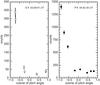 |
Fig. 5 Pitch angle distributions for the event. (left) Electrons with energies about 300 keV show very marked beam-like pitch angle distributions. (right) At a time consistent with the arrival of protons in the nominal energy range, P’8 shows also a very marked excess in count numbers from the sector corresponding to particles coming from the solar direction. |
Figure 4 shows the observed counts in P’2 integrated 144 s versus the observed counts in P’3 and P’8 (scaled so that they peak at about the same value). We subtracted the pre-event data. The fact that P’2 and P’3 very nearly show the same behavior is quite striking, as shown in Fig. 4. A simultaneous rise in the flux would not be enough to support the assumption of penetrating protons, since that could be explained by the spacecraft suddenly entering a region in space with higher pre-event fluxes. The different behavior in P’8, rising later than the channels that we know are more sensitive to higher energy penetrating ions (P’2, P’3), is a much stronger hint at the possibility that those counts are due to high energy protons. The value observed for P’2 (average of 10 counts per second between 02:00 and 02:10 UT) is consistent with that expected from NM data. Finally, the relative normalization, with P’2 counts roughly 1.5 times higher than those seen for P’3, is exactly what we would expect if those counts were dominated by protons with energies exceeding 1 GeV. We thus have strong evidence that P’2 and P’3 response extends to GeV energies and that those energies contribute significantly to the observed count rates.
The LAN2A telescopes use the spacecraft rotation to define eight look angles (sectors). For “field of view particles” entering through the aperture, the angle between the magnetic field and the detector normal corresponds to the pitch angle of arriving particles in each sector. Figure 5 (left) shows the pitch angle distributions measured for 300 keV electrons in LEFS60. The flux is strongly anisotropic and clearly peaks at the look angles corresponding to particles coming from Sun along a Parker spiral. A similar process is also seen for ions in LEMS120 after 04:00 UT, the time at which we expect the arrival of solar ions traveling from 6 to 10% of the speed of light (1874 to 4752 keV protons). As seen in Fig. 5 (right), the P’8 energy channel at 04:42 UT time shows very marked anisotropies consistent with a beam-like solar event. So we do see the signature of the solar event, as expected for nominal channel energies.
As shown in Fig. 6, things are very different for the early rise seen in the LEMS120 data. From the 02:10 UT flux versus direction plots in Fig. 6, one can see that the angular distribution of counts in both P’2 and P’8, although anisotropic, is nearly symmetric. Since we know the magnetic field, we can model the angular response from the detector expected for penetrating protons of different energies and compare it directly with EPAM data. This is shown by the dashed lines in Fig. 6. We assume that the protons are fully field aligned, as expected for the onset of a solar event, and we normalize the model to equal the total of the observed counts. To match the simulation results to observations, we had to assume that counts are dominated by particles higher than 1 GeV for P’2 and by less than 50 MeV for P’8; the agreement is then remarkable. Considering energies below 1 GeV for P’2 and above 50 MeV for P’8 significantly reduces the agreement between model response and observed directional counts. Figure 6 is again direct evidence that we are seeing penetrating protons, and the counts in P’2 are in great part due to protons with kinetic energies higher than 1 GeV. We note also that Fig. 6 being strikingly different from Fig. 5 discards one possibility that we had not yet addressed: the counts in LEMS120 might simply be due to contamination from high energy electrons that suffer less deflection at the magnets, and thus are able to reach M’.
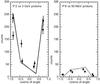 |
Fig. 6 Counts as a function of the angle between the magnetic field and the normal to the M’. The dashed line joins adjacent sectors, that is, marks the progression in time from sector to sector and is a model curve obtained from Monte Carlo simulations of the detector response for field aligned protons. (left) Model versus observation for P’2 measures, 2 min integration around 02:09:41 UT. (right) Model versus observation for P’8 measures, 10 minute integration after 02:09:41 UT. |
5. Threshold times and onset times
When looking into the timing of an in situ particle event one needs to distinguish between the time at which the event reaches a given threshold in the count rates, which are typically given as a function of signal-to-noise ratio or percentage of peak counts, and the time when the flux would have been seen starting to rise above the pre-event value in the absence of noise (the onset time). For “strong” events, when the threshold is a small fraction of maximum (less than 1%), corrections generally are not very relevant and the onset time can be assumed to be equal to the threshold time.
For many events, threshold times can only be readily computed from the available data at significant fractions of peak counts (10 to 20%) and inferring onset times require some assumptions regarding the shape of the rise in the count rates. Many factors affect this shape. Some of these factors relate to the acceleration and release of particles (short pulse versus complex injection at the source), others to propagation effects (pitch angle scattering prolongs the arrival of particles), and some are intrinsic to the instrument making the detection (look angles being sampled, range of energies being included in the same channel).
Propagation effects from the Sun to the Earth can be modeled using a focused transport approximation (Roelof 1969). For a very short injection (delta-functionlike) with the methods described in Maia et al. (2007), based on a scattering term from Kocharov et al. (1998), we have verified that the rise should be approximately linear from 1% up to 50% of the peak. A linear rise allows for a straightforward way to relate the onset time with the threshold time: one needs only to determine the time when the count rates (pre-event subtracted) reach a given (first) threshold and the time when they reach exactly twice that value. That length of time should then be subtracted from the first threshold time to obtain the onset time. The general case is not as straightforward. A complex injection with duration of minutes, and a broad response in energy surely complicates the picture, but the relevance of those two issues can be assessed by considering onset times inferred from consecutively higher thresholds.
5.1. Onset times at neutron monitor stations
Neutron monitor data do not give the omnidirectional flux, rathery they give essentially the flux from a particular look angle. Ideally, the omidirectional flux should be reconstructed using the available stations, but NMS located at sites sampling the small pitch angles should reasonably well reproduce the flux curve near the onset of the event. For 2012 May 17, Mishev et al. (2014) GLE show that the onset of the event is strongly anisotropic and it is clearly seen at Oulu, Apatity, and the South Pole, the stations corresponding to look directions with small pitch angles, and is rather weak at the other stations we studied. Even for the sites showing the strongest signal, data are quite noisy and require integration from 2 to 4 min to achieve a smooth rise.
The first step to determine an onset is to determine the optimal integration time. This requires both knowledge of the average slope of the event during the rise phase, and the noise at any given instant. To compute an average slope, we first determined the time to half-rise th , which is the time it took the event to rise from 20 to 70% of its peak value. For stations under consideration, th is below 10 minutes. For 2012 May 17, the rise from pre-event values is rather modest and the noise in the count rates can be assumed as constant. We note that NMS data needs to be pressure corrected, or there can be very large variations and underlying trends even at timescales of only a few hours. We used data from the day before the event to determine the noise levels and verified that the pre-event is reasonably stable and that a 4σ threshold is adequate to compute onset times.
To chose an integration time, we have used th to infer an average slope and then determined the time interval it would take an event for this kind of a slope to reach four times the pre-event noise levels. Apatity and Oulu thus required four-minute integration times; South Pole stations require integration times below 2.5 min. We then did a sliding average integration of the NMS data, subtracted the pre-event average values, and determined the time at which we first see a significant rise above the pre-event and the time at which we see the counts at twice that value. To determine biases that could be arising from the integration method used, and to assign error bars to the onsets thus computed, we ran 10 000 Monte Carlo simulations of onset determinations assuming a linear rise (same slope as the average computed for that particular NMS), the same pre-event noise function, and the same integration methods. The values obtained from those Monte Carlo simulations were then ordered and the median used as a correction (mostly negligible) for the onset time and percentiles corresponding to a standard variation for a normal distribution (approximately 16 and 84%) used to determine the uncertainty time ranges.
For Oulu data, the first threshold used for the linear approximation was 01:54.0 UT, corresponding to 4.1 times over pre-event background error and 25.2% of peak counts. The event took nearly four minutes to double the counts and as such the inferred onset time for Oulu data, using the linear approximation with correction for underlying biases, is 01:50.2 UT. The uncertainty interval is from 01:48.4 to 01:51.3 UT. The first threshold used for Apatity was at 19.8% of maximum, corresponding to 4.3 times over pre-event background error. The inferred onset time for Apatity, using the linear approximation with correction for underlying biases, is 01:49.6 UT. The uncertainty interval is from 01:47.9 to 01:50.6 UT. For South Pole and South Pole bare, we obtain statistically significant later times, 01:53.7 and 01:58.2 UT with uncertainties about ±1 mn from those values. The times we obtained are consistent with the values found in the literature. Li et al. (2013) using Oulu, Apatity, and the two South Pole stations determine an average onset time of 01:51 UT (±2 mn). Our average for the same four stations is 01:53 UT(±2 mn). Gopalswamy et al. (2013) used Oulu neutron monitor to determine that the onset at Earth took place between 01:38 to 01:45 UT. This is lower than our estimates for the same station although it can be accommodated at the 2σ level, particularly since the authors do not disclose how much smoothing was applied to the data. A variation such as the one encountered between different authors is not surprising given the reasonably large integration times required; all values are consistent within what we have found to be the optimal integration time (4 mn).
Apatity and Oulu are asymptotically close to each other and, as expected, the times we have obtained are consistent. South Pole values are clearly distinct and this could be because of a series of factors. There could be a slight difference in the pitch angles being sampled, but it is also possible that the South Pole detectors are recording a meaningful contribution of ions with lower energies than those sampled by Oulu and Apatity. For these four stations the effective cutoff rigidity is not determined by the geomagnetic cutoff but from atmospheric absorption. While Oulu is essentially at sea level (15 m altitude) and Apatity is not much higher (181 m altitude), South Pole stations are at 2820 m elevation above sea level. The response threshold of the neutron monitors to primary particles is about 430 MeV/nucleon for close to sea level stations, while for South Pole stations the reduced atmospheric mass lowers the threshold to ≈300 MeV/nucleon.
5.2. Onset times at EPAM
We determined the onset times for all LEMS120 channels although we only present the values for P’2 and P’8, since they define the extremes in instrumental temporal response. For the onset determinations, we removed the pre-event by detrending. The whole process of integration, biases and error assessment was similar to the one described for NMS data. Values for times to half-rise are about 27 min and optimal integration time was found to be 144 s. The fluctuations in the pre-event subtracted counts were slightly bigger than would be expected from count statistics alone, thus we determined the maximum and minimum values observed in detrended pre-event count values for the 90 min before 01:30 UT, and used the difference between those values as a limit to be exceeded by the threshold to be used. That is, we only considered times after the event crossed both the amplitude of fluctuations and had a signal-to-noise level of at least four. We used the first instance this condition was met and the time when that number of counts was doubled to compute the onset time, similar to our analysis of the NMS data. Since at this time we were only at a few percent of the peak in the counts, we were able to consider subsequent points and use each of those points as threshold for onset determination at different fractions of the peak in the counts.
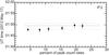 |
Fig. 7 Onset times versus percentage of peak for the P’2 channel. The dotted lines correspond to average (very close dots) and uncertainty range (more widely spaced dots) of onset times determined for the Apatity neutron monitor. |
Figure 7 shows how the inferred onset times in the linear approximation vary with the point used as the lower threshold for P’2. The rather short range of times seen for P’2 is quite striking; P’3 is not shown here but is very similar to the P’2 plot. The onset time computed for P’2 using 22 and 44% of peak flux as threshold levels are within the error bars of the value obtained for 4 and 8% of peak flux. This is consistent with a nearly linear rise. Figure 7 also compares the EPAM times with the value found for Apatity neutron monitor. The agreement is remarkable. The first determination for P’2 gives 01:47.9 UT as onset time, with an uncertainty time interval from 01:47.1 to 01:48.5 UT.
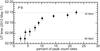 |
Fig. 8 Onset times versus percentage of peak for the P’8 channel. The dotted lines correspond to times when energies of 35 and 90 MeV would reach the Earth orbit assuming that the onset times measured for P’2 reflect the arrival of 3 GeV protons. |
Mishev et al. (2014) determined the energy spectra from the NMS data as the event progresses, and from their analysis we can infer that, during the GLE, fluxes from solar particles of rigidity higher than about 4 GV are not seen above Galactic cosmic ray values. For protons, this corresponds to a kinetic energy of about 3.1 GeV. From the spectra presented in Mishev et al. (2014) and from our model results we also verified that we still expect a small but significant number of counts at energies higher than 3.1 GeV, so we assign that energy as being the limit for detectability in P’2. Since counts numbers are higher in P’2 than P’3, we can then bound the response in P’2 as being due to at least 1 GeV protons. From the solar wind for this day we compute a spiral magnetic field length from the sun to the earth of 1.20 AU, and from that we infer that 3.1 GeV protons left the Sun at about 01:37.7 UT, and that the uncertainty in the exact energy range does not lower this value by more than one minute.
As shown in Fig. 8 for P’8 the values for the onset computed from different fractions of the peak count rates span about 15 min in time. The dotted lines in Fig. 8 show the arrival times expected for protons of 35 and 90 MeV, assuming they left the Sun at 01:37.7 UT. Although the channel count rates rise in a way that clearly is not linear, the computed onset times determined using different thresholds of the peak in the counts are bound by what we expect to be the likely energy range for the channel. For P’8, we were also able to determine the onset of ions in the nominal energy range identifying the onset from its signature in flux angular signatures (illustrated in Fig. 5).
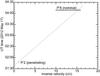 |
Fig. 9 Arrival times for P’2 penetrating ions, whose counts are dominated by higher than 1 GeV protons, and for P’8 field of view 1.9 to 4.8 MeV per nucleon ions. The dashed line marks the expected arrival time at 1 AU as a function of inverse velocity for particles released back at the Sun at 01:37.7 UT and following the archimedian spiral corresponding to the observed solar wind conditions. |
6. Discussion and conclusions
We identified a signature in the LEMS120 ion telescopes in EPAM, which can be attributed to penetrating high energy protons entering the detector chamber and being counted in the nominal low energy channels. The inferred energies and onset times agree very well with neutron monitor stations close to sea level like Apatity and Oulu and are consistent with the first arriving particles having energies from 1 to 3 GeV. The high energy signatures detected in the EPAM data are relatively easy to identify: onset at ion channels almost at the same time as the onset for the electron channels, with the onset at P’2 and P’3 earlier than for P’8, marked anisotropies in the pitch angle distribution with shapes differing strongly between P’2 and P’8. This development offers another valuable source of information for many other ion events that occurred after the launch of EPAM. We verified that other GLEs, including the particularly strong event on 2005 January 20, show the same type of signatures. The prospect of being able to study near relativistic proton events also offers a reason to reexamine HISCALE data to look for GLE-like events that might have missed the Earth.
The 2012 May 17 GLE is particularly interesting for two main reasons: (i) it is only the first of solar cycle 24, while in the same period of solar cycle 23 five had already been seen; and (ii) it is related to a rather mild flare, only M class. There are already a few articles published on the timing of the electrons and ions seen in association with the 2012 May 17 GLE and how those relate to the flare and CME activity (Gopalswamy et al. 2013; Li et al. 2013). We were able to significantly constrain the inferred release time for the ions back at the Sun because P’2 is dominated by a relatively narrow range in propagation times (protons with velocities between 0.9 and 0.97c). Figure 9 compares the onset times determined for P’2 (penetrating protons) and P’8 (1.9 to 4.8 MeV nominal energy ions). The determined onset times are consistent when one considers the full range of energy for the channels, so that the first arriving 2−5 MeV and higher than 1 GeV ions could have been accelerated in related processes. The P’2 onset timing implies a release back at the Sun of about 01:37.7 UT for the ions; the corresponding electromagnetic emissions that could help identify the source region of those particles would arrive at the Earth at 01:46 UT.
The GLE was associated with an M5.1 flare starting, peaking, and ending at 01:25, 01:47, and 02:14 UT, respectively. Gopalswamy et al. (2013) report also a metric type II burst at 01:32 UT by directly examining the dynamic spectra from Hiraiso, Culgoora, and Learmonth observatories. These times should be compared with 01:46 UT, when we would expect to see electromagnetic signatures from the Sun at 1 AU associated temporally with the ion release. Both the flare start and the type II onset occur well before the time inferred for the ion release. Gopalswamy et al. (2013) present a thorough analysis of the timing of the fast CME associated with the GLE event, using coronagraphic data and from that analysis we can infer that the ions were released after the CME initiation when the CME leading edge was about 3 solar radii from Sun center. Gopalswamy et al. (2013) attribute the ion event to acceleration by a CME driven shock, developing low in the corona. However, the fact that the time we infer for the ion release nearly coincides with the peak in soft X-ray emission, which can be used, although with some caution, as a proxy for the end of hard X-ray emission, is intriguing. We can not thus completely exclude that the origin of GeV ions could be related to a magnetic restructuring process back at Sun such that the (weak) emission from precipitating particles confined inside closed structures suddenly ceased when particles gained access to open field lines, thus being able to reach 1 AU.
Acknowledgments
The authors thank the work and dedication of the Ulysses HISCALE team, and acknowledge having used reference documentation authored by S.J. Tappin, E. Roelof, D. Haggerty and T.P. Armstrong. This work was made possible in part by NASA and ESA through the Ulysses/HISCALE project, and by NASA through the ACE/EPAM project.
References
- Geant4 Collaboration, Agostinelli, S., Allison, J., et al. 2003, Nucl. Instr. Meth. Phys. Res. A, 506, 250 [Google Scholar]
- Gold, R. E., Krimigis, S. M., Hawkins, III, S. E., et al. 1998, Space Sci. Rev., 86, 541 [Google Scholar]
- Gopalswamy, N., Xie, H., Akiyama, S., et al. 2013, ApJ, 765, L30 [NASA ADS] [CrossRef] [Google Scholar]
- Haggerty, D. K., & Roelof, E. C. 2006, Adv. Space Res., 38, 990 [NASA ADS] [CrossRef] [Google Scholar]
- Haggerty, D. K., Roelof, E. C., Ho, G. C., & Gold, R. E. 2006, Adv. Space Res., 38, 995 [NASA ADS] [CrossRef] [Google Scholar]
- Kocharov, L., Vainio, R., Kovaltsov, G. A., & Torsti, J. 1998, Sol. Phys., 182, 195 [NASA ADS] [CrossRef] [Google Scholar]
- Lanzerotti, L. J., Gold, R. E., Anderson, K. A., et al. 1992, A&AS, 92, 349 [NASA ADS] [Google Scholar]
- Li, C., Firoz, K. A., Sun, L. P., & Miroshnichenko, L. I. 2013, ApJ, 770, 34 [Google Scholar]
- Maia, D. J. F., Gama, R., Mercier, C., et al. 2007, ApJ, 660, 874 [NASA ADS] [CrossRef] [Google Scholar]
- Mishev, A. L., Kocharov, L. G., & Usoskin, I. G. 2014, J. Geophys. Res. (Space Phys.), 119, 670 [Google Scholar]
- Patterson, J. D., & Armstrong, T. P. 2001, Determination of HISCALE MFSA Background Rates Using IMP-8 Monitored Omnidirectional Galactic Cosmic Rays, Tech. Rep. LLC, Memorandum, Fundamental Technologies [Google Scholar]
- Patterson, J. D., & Armstrong, T. P. 2003, Geophys. Res. Lett., 30, 8037 [NASA ADS] [CrossRef] [Google Scholar]
- Peltola, T. 2014, J. Instrum., 9, C2010 [CrossRef] [Google Scholar]
- Roelof, E. C. 1969, in Lectures in High-Energy Astrophysics, eds. H. Ögelman, & J. R. Wayland, 111 [Google Scholar]
- Wüest, M., Evans, D. S., & von Steiger, R. 2007, Calibration of Particle Instruments in Space Physics (ESA Communications for the International Space Science Institute) [Google Scholar]
All Tables
All Figures
|
Fig. 1 LAN2A assembly of the EPAM instrument, formed by the LEMS120 and LEFS60 telescopes. |
| In the text | |
|
Fig. 2 Results from Monte Carlo simulations showing number of particles versus deposited energy for two incident proton energies. A million protons were simulated at each energy, propagating parallel to the detector normal and impacting the center of the detector; the gray band marks the energy range corresponding to P’2. |
| In the text | |
|
Fig. 3 Results from Monte Carlo simulations of protons hitting M’, showing the relative response, under the form of geometrical factors, of channels P’2 (thin full line), P’3 (thick full line), and P’8 (dashed line). |
| In the text | |
|
Fig. 4 Comparison of the counts from the LEMS120 P’2, P’3, and P’8 counts for 144 s integrations. Counts from P’3 and P’8 have been scaled so that the peak counts for all channels are at equivalent levels. |
| In the text | |
|
Fig. 5 Pitch angle distributions for the event. (left) Electrons with energies about 300 keV show very marked beam-like pitch angle distributions. (right) At a time consistent with the arrival of protons in the nominal energy range, P’8 shows also a very marked excess in count numbers from the sector corresponding to particles coming from the solar direction. |
| In the text | |
|
Fig. 6 Counts as a function of the angle between the magnetic field and the normal to the M’. The dashed line joins adjacent sectors, that is, marks the progression in time from sector to sector and is a model curve obtained from Monte Carlo simulations of the detector response for field aligned protons. (left) Model versus observation for P’2 measures, 2 min integration around 02:09:41 UT. (right) Model versus observation for P’8 measures, 10 minute integration after 02:09:41 UT. |
| In the text | |
|
Fig. 7 Onset times versus percentage of peak for the P’2 channel. The dotted lines correspond to average (very close dots) and uncertainty range (more widely spaced dots) of onset times determined for the Apatity neutron monitor. |
| In the text | |
|
Fig. 8 Onset times versus percentage of peak for the P’8 channel. The dotted lines correspond to times when energies of 35 and 90 MeV would reach the Earth orbit assuming that the onset times measured for P’2 reflect the arrival of 3 GeV protons. |
| In the text | |
|
Fig. 9 Arrival times for P’2 penetrating ions, whose counts are dominated by higher than 1 GeV protons, and for P’8 field of view 1.9 to 4.8 MeV per nucleon ions. The dashed line marks the expected arrival time at 1 AU as a function of inverse velocity for particles released back at the Sun at 01:37.7 UT and following the archimedian spiral corresponding to the observed solar wind conditions. |
| In the text | |
Current usage metrics show cumulative count of Article Views (full-text article views including HTML views, PDF and ePub downloads, according to the available data) and Abstracts Views on Vision4Press platform.
Data correspond to usage on the plateform after 2015. The current usage metrics is available 48-96 hours after online publication and is updated daily on week days.
Initial download of the metrics may take a while.