| Issue |
A&A
Volume 577, May 2015
|
|
|---|---|---|
| Article Number | A60 | |
| Number of page(s) | 6 | |
| Section | Stellar structure and evolution | |
| DOI | https://doi.org/10.1051/0004-6361/201525812 | |
| Published online | 05 May 2015 | |
Stellar models with mixing length and T(τ) relations calibrated on 3D convection simulations
1
Astrophysics Research Institute, Liverpool John Moores
University,
IC2, Liverpool Science Park, 146 Brownlow
Hill,
Liverpool
L3 5RF,
UK
e-mail:
M.Salaris@ljmu.ac.uk
2
INAF−Osservatorio Astronomico di Collurania, via M.
Maggini, 64100
Teramo,
Italy
e-mail:
cassisi@oa-teramo.inaf.it
Received: 5 February 2015
Accepted: 13 March 2015
The calculation of the thermal stratification in the superadiabatic layers of stellar models with convective envelopes is a long-standing problem of stellar astrophysics, and has a major impact on predicted observational properties such as radius and effective temperature. The mixing length theory, almost universally used to model the superadiabatic convective layers, contains one free parameter to be calibrated (αml) whose value controls the resulting effective temperature. Here we present the first self-consistent stellar evolution models calculated by employing the atmospheric temperature stratification, Rosseland opacities, and calibrated variable αml (dependent on effective temperature and surface gravity) from a recently published large suite of three-dimensional radiation hydrodynamics simulations of stellar convective envelopes and atmospheres for solar stellar composition. From our calculations (with the same composition of the radiation hydrodynamics simulations), we find that the effective temperatures of models with the hydro-calibrated variable αml (that ranges between ~1.6 and ~2.0 in the parameter space covered by the simulations) present only minor differences, by at most ~30–50 K, compared to models calculated at constant solar αml (equal to 1.76, as obtained from the same simulations). The depth of the convective regions is essentially the same in both cases. We also analyzed the role played by the hydro-calibrated T(τ) relationships in determining the evolution of the model effective temperatures, when compared to alternative T(τ) relationships often used in stellar model computations. The choice of the T(τ) can have a larger impact than the use of a variable αml compared to a constant solar value. We found that the solar semi-empirical T(τ) by Vernazza et al. (1981, ApJS, 45, 635) provides stellar model effective temperatures that agree quite well with the results with the hydro-calibrated relationships.
Key words: convection / stars: evolution / Hertzsprung-Russell and C-M diagrams
© ESO, 2015
1. Introduction
The almost universally adopted method for calculating superadiabatic convective temperature gradients in stellar evolution models is based on the formalism provided by the mixing length theory (MLT; Böhm-Vitense 1958). This formalism is extremely simple; the gas flow is made of columns of upward and downward moving convective elements with a characteristic size, the same in all dimensions, that cover a fixed mean free path before dissolving. All convective elements have the same physical properties at a given distance from the star centre; upward moving elements release their excess heat into the surrounding gas, and are replaced at their starting point by the downward moving elements that thermalize with the surrounding matter, thus perpetuating the cycle. The MLT is a local theory, and the evaluation of all relevant physical and chemical quantities are based on the local properties of each specific stellar layer, regardless of the extension of the whole convective region.
Both the mean free path and the characteristic size of the convective elements are assumed to be same for all convective bubbles, and are assigned the same value Λ = αmlHp, the mixing length. Here αml is a free parameter (assumed to be a constant value within the convective regions and along all evolutionary phases), and Hp is the local pressure scale height. There are additional free parameters in the MLT that are generally fixed a priori (versions of the MLT with different choices of these additional parameters will be denoted here as different MLT flavours), so that practically the only free parameter to be calibrated is αml. Stellar evolution calculations for a fixed mass and initial chemical composition but with varying αml produce evolutionary tracks with different Teff and radius evolution, whereas evolutionary timescales and luminosities are typically unchanged. On the other hand, the prediction of accurate values of Teff and radii by evolutionary models and stellar isochrones is paramount to the study of colour–magnitude diagrams of resolved stellar populations, empirical mass-radius relations of eclipsing binary systems, and predicting reliable integrated spectra and colours of unresolved stellar systems (extragalactic clusters and galaxies).
In stellar evolution calculations the value of αml is usually calibrated by reproducing the radius of the Sun at the solar age with an evolutionary solar model. This solar calibrated αml is then kept fixed in all evolutionary calculations of stars of different masses and chemical compositions. The exact numerical value of αml varies amongst calculations by different authors because variations of input physics and choices of the outer boundary conditions affect the predicted model radii and Teff values, hence require different αml values to match the Sun. Pedersen et al. (1990) and Salaris & Cassisi (2008) have shown how the various MLT flavours provide the same Teff evolution once αml is appropriately recalibrated on the Sun.
As discussed by e.g. Vandenberg et al. (1996) and Salaris et al. (2002), metal-poor red giant branch (RGB) models calculated with the solar calibrated value of αml (hereafter αml, ⊙) are able to reproduce the Teff of samples of RGB stars in Galactic globular clusters within the error bars on the estimated Teff. On the other hand, several authors find that variations of αml with respect to αml, ⊙ are necessary to reproduce – to give some examples – the red edge of the RGB in a sample of 38 nearby Galactic disc stars with radii determined from interferometry (Piau et al. 2011); the asteroseismically constrained radii of a sample of main sequence (MS) Kepler targets (Mathur et al. 2012); observations of binary MS stars in the Hyades (Yıldız et al. 2006); and the α Cen system (Yıldız 2007), a low-mass pre-MS eclipsing binary in Orion (Stassun et al. 2004).
The MLT formalism only provides a very simplified description of convection, and there have been several attempts to introduce non-locality in the MLT (see e.g. Grossman et al. 1993; Deng et al. 2006, and references therein). These refinements of the MLT are often complex and introduce additional free parameters to be calibrated. The alternative model by Canuto & Mazzitelli (1991, 1992) includes a spectrum of eddy sizes (rather than the one-sized convective cells of the MLT) and fixes the scale length of the convective motions to the distance to the closest convective boundary. Recently Pasetto et al. (2014) have presented a new non-local and time-dependent model based on the solution of the Navier-Stokes equations for an incompressible perfect fluid that does not contain any free parameters1.
An alternative approach to modelling the superadiabatic layers of convective envelopes is based on the computation of realistic multidimensional radiation hydrodynamics (RHD) simulations of atmospheres and convective envelopes – where convection emerges from first principles – that cover the range of effective temperatures (Teff), surface gravities (g), and compositions typical of stars with surface convection. These simulations have reached a high level of sophistication (see e.g. Nordlund et al. 2009), and for ease of implementation in stellar evolution codes their results can be used to provide an hydro-calibration of an effective αml, even though RHD simulations do not confirm the basic MLT picture of columns of convective cells. After early attempts using rather crude two-dimensional (2D) and three-dimensional (3D) simulations (see e.g. Deupree & Varner 1980; Lydon et al. 1992), a first comprehensive RHD calibration of αml was presented by Ludwig et al. (1999) and Freytag et al. (1999). These authors found from their simulations that the calibrated αml varies as a function of metallicity, g and Teff. Freytag & Salaris (1999) applied this RHD calibration of αml (plus T(τ) relations computed from the same RHD models, and Rosseland opacities consistent with the RHD calculations) to metal-poor stellar evolution models for Galactic globular cluster stars, and found that the resulting isochrones for the relevant age range have only small Teff differences along the RGB (of the order of ~50 K) compared to isochrones computed with a solar calibrated value of αml.
In recent years a number of grids of 3D hydrodynamics simulations of surface convection have been published, and from the point of view of stellar model calculations it is very important to study whether the results by Freytag & Salaris (1999) are confirmed or drastically changed.
Tanner et al. (2013b,a) have presented a grid of simulations employing a 3D Eddington solver in the optically thin layers (Tanner et al. 2012). Their calculations cover four metallicities (from Z = 0.001 to Z = 0.04), but just a few Teff values at constant log(g) = 4.30 for each Z, plus a subset of models at varying He mass fraction for Z = 0.001 and Z = 0.02. These authors studied the properties of convection with varying Teff and chemical composition in these solar-like envelopes. Tanner et al. (2014) extracted metallicity-dependent T(τ) relations from these same simulations, and employed them to highlight the critical role these relations play when calibrating αml with stellar evolution models.
Magic et al. (2013) have published a very large grid of 3D RHD simulations for a range of chemical compositions. Their grid covers a range of Teff from 4000 to 7000 K in steps of 500 K, a range of log(g) from 1.5 to 5.0 in steps of 0.5 dex, and metallicity, [Fe/H], from −4.0 to +0.5 in steps of 0.5 and 1.0 dex. These models have been employed by Magic et al. (2015) to calibrate αml as function of g, Teff, and [Fe/H]. They found that αml depends in a complex way on these three parameters, but in general αml decreases towards higher effective temperature, lower surface gravity, and higher metallicity. So far Magic et al. (2015) have only provided fitting formulae for αml, but not publicly available prescriptions for the boundary conditions and input physics.
Very recently Trampedach et al. (2013) produced a non-square grid of convective atmosphere/envelope 3D RHD simulations for the solar chemical composition. The grid spans a Teff range from 4200 to 6900 K for MS stars around log(g) = 4.5, and from 4300 to 5000 K for red giants with log(g) = 2.2, the lowest surface gravity available. In Trampedach et al. (2014b) the horizontal and temporal averages of the 3D simulations were then matched to 1D hydrostatic equilibrium, spherically symmetric envelope models to calibrate αml as a function of g and Teff (see Trampedach et al. 2014b, for details about the calibration procedure). Moreover, the same RHD simulations have been employed by Trampedach et al. (2014a) to calculate g- and Teff-dependent T(τ) relations from temporal and τ (Rosseland optical depth) averaged temperatures of the atmospheric layers. Trampedach et al. (2014b) also provide routines for calculating their g- and Teff-dependent RHD-calibrated αml together with their computed T(τ) relations, and Rosseland opacities consistent with the opacities used in the RHD simulations. This enables stellar evolution calculations where boundary conditions, superadiabatic temperature gradients and opacities of the convective envelope are consistent with the RHD simulations. It is particularly important to use both the RHD-calibrated αml and T(τ) relations because the Teff of the stellar evolution calculations depends on both these inputs (see e.g. Salaris et al. 2002; Tanner et al. 2014, and references therein).
Thanks to this consistency between RHD simulations and publicly available stellar model inputs, we present and discuss in this paper the first stellar evolution calculations where the Trampedach et al. (2014b) 3D RHD-calibration of αml is self-consistently included in the evolutionary code. In the same vein as Freytag & Salaris (1999), we focus on the effect of the calibrated variable αml on the model Teff, compared to the case of calculations with fixed αml, ⊙ (as determined from the same RHD simulations). Self-consistency of opacity and boundary conditions is paramount in order to assess correctly differential effects, given that the response of models to variations of αml depends on their Teff, which in turn depends on the absolute value of αml, opacities, and boundary conditions. We also address the role played by the RHD calibrated T(τ) relations in the determination of the model Teff when compared to other widely used relations.
Section 2 briefly describes the relevant input physics of the models, while Sect. 3 presents and compares the resulting evolutionary tracks. A summary and discussion close the paper.
2. Input physics
All stellar evolution calculations presented here were performed with the BaSTI (BAg of Stellar Tracks and Isochrones) code (Pietrinferni et al. 2004) for a chemical composition with Y = 0.245, Z = 0.018, and the Grevesse & Noels (1993) metal mixture consistent with the chemical composition of the RHD simulations. Atomic diffusion was switched off in these calculations, and convective core overshooting was included when appropriate (see Pietrinferni et al. 2004, for details).
We employed the Rosseland opacities provided by Trampedach et al. (2014b). The low temperature opacities (for log(T) < 4.5) are very close to Ferguson et al. (2005) with the exception of the region with log(T) < 3.5, where the Ferguson et al. (2005) calculations are higher because of the inclusion of the effect of water molecules (see Trampedach et al. 2014a). Opacity Project (Badnell et al. 2005) calculations are used for log(T) ≥ 4.5. Regarding the surface boundary conditions, we employed the T(τ) relations computed by Trampedach et al. (2014a), who provided a routine that calculates, for a given Teff and surface gravity, the appropriate generalized Hopf functions q(τ) related to the T(τ) relation by 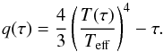 (1)In our calculations we fixed at τtr = 2/3 the transition from the T(τ) integration of the atmospheric layers (with τ as independent variable) to the integration of the full system of stellar structure equations. As mentioned by Trampedach et al. (2014a,b), these RHD-based T(τ) relations can also be employed to model the convective layers in the optically thick part of the envelope, together with modified expressions for the temperature gradients in the superadiabatic regions, and an appropriate rescaling of τ (see Trampedach et al. 2014a, for details). In our calculations we compared the radiative (∇rad) and superadiabatic (∇, obtained with the RHD calibrated values of αml) temperature gradients determined along the upper part of the convective envelopes from the standard stellar structure equations and MLT (down to τ = 100, the upper limit for the routine calculating the Hopf functions), with ∇rad and ∇ calculated according to Eqs. (35) and (36) of Trampedach et al. (2014a), respectively. We have found that in all our models the differences between these two sets of gradients are much less than 1% between τtr and τ = 100.
We also calculated test models by changing τtr between 2/3 and 5 (with the appropriate rescaling of τ if convection appears in the atmosphere integration, see Trampedach et al. 2014a), and obtained identical evolutionary tracks in each case.
Regarding the value of αml, the same routine for the Hopf functions also provides the RHD calibrated value of αml (for the Böhm-Vitense 1958, flavour of the MLT) for a given Teff and surface gravity that we employed in our calculations. Uncertainties in the calibrated αml values are of the order of ± 0.02−0.03 (see Table 1 of Trampedach et al. 2014b)2.
The only difference in terms of input physics between the atmosphere/envelope RHD calculations and our models is the equation of state (EOS). The RHD simulations employed the MHD (Daeppen et al. 1988) EOS, which is not the same EOS used in the BaSTI calculations (see Pietrinferni et al. 2004). To check whether this can cause major differences in the models, we calculated envelope models for the same g − Teff pairs of the RHD simulations, including the RHD-calibrated αml, T(τ) relations, and RHD opacities. We then compared the resulting depths of the convection zones (dCZ, in units of stellar radius) with the values obtained by Trampedach et al. (2014b) from their RHD-calibrated 1D envelope models, which used the same input physics (including EOS) of the RHD calculations (see Table 1 of Trampedach et al. 2014b). We found random (non-systematic) differences of dCZ by at most just 2–3% compared to the Trampedach et al. (2014b) results.
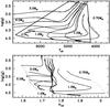 |
Fig. 1 Stellar evolution tracks in the g − Teff diagram for the labelled masses. The region enclosed by the thick black boundary is the g − Teff range covered by the RHD simulations. Thick solid lines denote fully consistent calculations with the RHD calibrated variable αml and T(τ) relationships. The lower panel displays the evolution of αml along each track. The dotted portion of each sequence denotes the region where the αml values are extrapolated. Dashed lines in the upper panel represent tracks calculated with a constant αml = αml, ⊙ and the RHD T(τ) relationships. |
3. Model comparisons
As mentioned in the introduction, the RHD simulations cover a non-square region in the g − Teff diagram, as shown in Fig. 1 (the region enclosed by thick solid lines), ranging from 4200 to 6900 K on the MS, and from 4300 to 5000 K for RGB stars with log(g) = 2.2. The MLT calibration results in an αml varying from 1.6 for the warmest dwarfs, with a thin convective envelope, up to 2.05 for the coolest dwarfs in the grid. In between there is a triangular plateau of αml ~ 1.76, where the Sun is located. The RHD simulation for the Sun provides αml ~ 1.76 ± 0.03. The top panel of Fig. 1 shows the results of our evolutionary model calculations in the g − Teff diagram (from the pre-MS to the lower RGB), for masses M = 0.75, 1.0, 1.4, 2.0, and 3.0 M⊙ that cover the full domain of the RHD simulations.
The thick solid lines denote the reference set of models, calculated with the varying αml calibration, and the run of αml along each individual track is shown in the lower panel. The dotted part of each sequence in this panel denotes the αml values extrapolated by the calibration routine, when the models are outside the region covered by the simulations but still retain a convective region. This happens along the pre-MS evolution of the M = 0.75 M⊙ track, and for the 2.0 and 3.0 M⊙ calculations along the subgiant phase. Apart from the pre-MS stages of the two lowest mass models, the evolution of αml spans a narrow range of values, between ~1.6 and ~1.8.
To study the significance of the variation of αml for the model Teff, we calculated evolutionary models for the same masses, this time keeping αml = αml, ⊙ = 1.76 along the whole evolution. The results are also shown in Fig. 1.
A comparison of the two sets of tracks clearly shows that the effect of a varying αml is almost negligible. The largest differences are of only ~30 K along the RGB phase of the 3.0 M⊙ track (solar  tracks being hotter because of a higher αml value compared to the calibration) and ~50 K at the bottom of the Hayashi track of the 1.0 M⊙ track (solar αml tracks being cooler because of a lower αml). In all other cases differences are smaller, often almost zero.
For all stellar masses we found that the mass fraction of He dredged to the surface by the first dredge up, which depends on the maximum depth of the convective envelope at the beginning of the RGB phase, is the same within 0.001 between constant αml, ⊙ and variable αml models. We then compared the luminosity of the RGB bump, which also depends on the maximum depth of the convective envelope at the first dredge up (see e.g. Cassisi & Salaris 1997, 2013, and references therein), for the 0.75 and 1.0 M⊙ models. We found that the luminosity is unchanged between models with constant and variable αml. This reflect the fact that the depth of the convective envelope is the same between the two sets of models throughout the MS phase to the RGB until the end of the calculations. Small differences appear only during the pre-MS. To this purpose, for the 1.0 M⊙ models we additionally checked the surface Li abundance that survives the pre-MS depletion. This provides information about the evolution of the lower boundary of the convective envelope during this phase, where according to Fig. 1, αml shows the largest difference from αml, ⊙. We found that, after the pre-MS, models with constant αml, ⊙ display a Li abundance just 9% higher than the reference results.
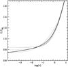 |
Fig. 2 Comparison of the ratio T/Teff as a function of the optical depth τ as predicted by different T(τ) relationships. The thick solid and dotted lines represent the RHD-calibrated relationships for Teff = 4500 K and 6000 K (log(g) = 3.5 in both cases), respectively. The thin solid, dash-dotted, and dashed lines show the ratios obtained from the Eddington, KS, and VALcT(τ) relationships, respectively. |
We then analyzed the role played by the T(τ) relationships computed from the RHD calculations in determining the model Teff (the role played by the boundary conditions in determining the Teff of stellar models is especially crucial for very low-mass stars, see e.g. Allard et al. 1997; Brocato et al. 1998). Figure 2 shows the ratio T/Teff as a function of τ as predicted by the calibrated relationships for atmospheres/envelopes with Teff = 4500 K and 6000 K (log(g) = 3.5). The RHD calibrated T(τ) relationships contain values for the Hopf function that vary with τ and Teff (also with g, but to a lesser degree). The variation with Teff is obvious from the figure. For these two temperatures the largest differences appear at the layers with τ between ~0.1 and ~−1, where stellar model calculations usually fix the transition from the atmosphere to the interior. Figure 2 also shows the results of the traditional Eddington approximation to the grey atmosphere, and the solar semi-empirical T(τ) relationships by Krishna-Swamy (KS; Krishna Swamy 1966) and Vernazza et al. (1981) – their Model C for the quiet sun, hereafter VALcT(τ). In these cases the ratio T/Teff does not depend on Teff. It is easy to notice that around the photospheric layers the RHD relationships are in between the Eddington grey and VALcT(τ). The most discrepant relationship is the KS one.
 |
Fig. 3 As the upper panel of Fig. 1 but for evolutionary tracks with masses equal to 1.0 and 1.4 M⊙, respectively. Thick solid lines denote fully consistent calculations with the RHD calibrated variable αml and T(τ) relationships. Dotted, dash-dotted, and dashed lines display tracks calculated with constant αml, ⊙ and the Eddington, KS, and VALcT(τ), respectively. |
Figure 3 shows the results of evolutionary calculations with this set of T(τ) relationships. We compare here the reference set of models for 1.0 and 1.4 M⊙ and varying αml, with constant αml, ⊙ models calculated using the Eddington, KS, and VALcT(τ) relationships (τtr = 2/3 also for these calculations).
The differences between these new sets of models at constant αml, ⊙ and the reference calculations are larger than the case of Fig. 1 because of the differences with the RHD T(τ) relationships. On the whole, the VALcT(τ) (coupled to the RHD calibrated αml, ⊙) gives the closest match to the self-consistent reference calculations. The largest differences appear for the 1.0 M⊙ along the pre-MS; models calculated with the VALc relation are ~50 K cooler, approximately the same as the case of αml, ⊙ and the RHD T(τ). For the same 1.0 M⊙ track the Teff differences along the RGB are at most 10 K, and at most ~40 K along the MS. Differences for the 1.4 M⊙ track are smaller.
Regarding the Eddington T(τ), the resulting tracks are generally hotter than the self-consistent RHD-based calculations. The largest differences amount to ~40–50 K along MS and RGB of the two tracks. Comparisons with Fig. 1 show that, from the point of view of the resulting model Teff, the Eddington T(τ) differs more – although not by much – than the VALc one from the RHD relations.
The worse agreement is found with the KS T(τ). For both masses the RGB is systematically cooler by ~70 K, and the pre-MS by ~80–100 K, whilst the MS of the 1.0 M⊙ calculations is cooler by ~120 K, a difference reduced to ~50 K along the MS of the 1.4 M⊙ track.
In case of the 1.0 M⊙ models we rechecked the luminosity level of the RGB bump, the surface He mass fraction after the first dredge up, and the amount of surface Li after the pre-MS depletion. For all these three T(τ) relations the evolutionary models display a RGB bump luminosity within Δ(L/L⊙) < 0.01, and a post-dredge up He abundance within 0.001 of the fully consistent result. In all these calculations the convective envelope has the same depth throughout the MS phase and along the RGB. Differences along the pre-MS are highlighted by the amount of Li depletion during this phase. We found that models calculated with the Eddington T(τ) have 9% less Li after the pre-MS than the reference calculations. Comparing this number with just the effect of a constant αml, ⊙ discussed above, we derive that the use of this T(τ) decreases the surface Li abundance by ~20% compared to the use of the Hopf functions determined from the RHD simulations. In the case of the VALcT(τ), the net effect is to increase the surface Li after the pre-MS by ~10% compared to the RHD T(τ), and the KS relation causes a similar increase by ~11%.
3.1. The standard solar model
We close our analysis by discussing the implications of the RHD results and the choice of the T(τ) relation, on the calibration of the standard solar model. As is well known, in stellar evolution it is customary to fix the value of αml, ⊙ (and the initial solar He and metal mass fractions) by calculating a 1 M⊙ stellar model that matches the solar bolometric luminosity and radius at the age of the Sun, with the additional constraint of reproducing the present metal to hydrogen mass fraction Z/X ratio (see e.g. Pietrinferni et al. 2004, for details). The accuracy of the derived solar model can then be tested against helioseismic estimates of the depth of the convective envelope and the surface He mass fraction. It is also well established that solar models without microscopic diffusion cannot properly account for some helioseismic constraints, hence solar models are routinely calculated by including microscopic diffusion of He and metals (see e.g. Pietrinferni et al. 2004, for a discussion and references).
We first calculated a standard solar model (with the same input physics and solar metal distribution of the calculations discussed above) employing both the variable αml and the T(τ) relations from the RHD results. Given that microscopic diffusion decreases the surface chemical abundances of the model with time, the initial solar Z (and Y) need to be higher than the present level. This means that we also had to employ the RHD results for chemical compositions that were not exactly the same as the composition of the RHD simulations.
We found that it is necessary to rescale the RHD αml calibration by a factor of just 1.034 to reproduce the solar radius. This implies αml, ⊙ = 1.82, extremely close, within the error, to the RHD value αml, ⊙ = 1.76 ± 0.01(range) ±0.03(calibration uncertainty) obtained by Trampedach et al. (2014b). Given our previous results, it is also obvious that a solar model calibration with fixed αml and the RHD T(τ) relations provides the same αml, ⊙ = 1.82.
Solar calibrations with the KS, VALc, and Eddington T(τ) relations have provided αml, ⊙ = 2.11, 1.90, and 1.69, respectively.
In all these calibrated solar models the initial solar He mass fraction (Yini, ⊙ ~ 0.274) and metallicity ((Zini, ⊙ ~ 0.0199) are essentially the same, as expected. In addition, the model values for the present He mass fraction in the envelope (Y⊙ = 0.244) and the depth of the convection zone (dCZ = 0.286R⊙) are the same for all calibrations and are in agreement with the helioseismic values (see e.g. Dziembowski et al. 1995; Basu & Antia 1997).
If we take αml, ⊙ obtained with the RHD T(τ) as a reference, the lower value obtained with the Eddington T(τ) and the larger values obtained with both the VALc and KS relations (in increasing order) are fully consistent with the results of Fig. 3. In that figure VALc and KS T(τ) MS models are increasingly cooler than the reference RHD calculations (hence increasingly larger αml values are required to match the reference MS) whereas the use of the Eddington T(τ) produces models hotter than the reference MS (hence lower αml value are needed to match the reference MS).
4. Summary and discussion
We presented the first self-consistent stellar evolution calculations that employ the variable αml and T(τ) by Trampedach et al. (2014b), based on their 3D RHD simulations. Our set of evolutionary tracks for different masses and the same chemical composition (plus consistent Rosseland opacities) of the RHD simulations, cover approximately the entire g − Teff parameter space of the 3D atmosphere/envelope calculations.
We found that, from the point of view of the predicted Teff (plus the depth of the convective envelopes and amount of pre-MS Li depletion), models calculated with constant RHD calibrated αml, ⊙ = 1.76 are very close to, and often indistinguishable from, the models with variable αml. The maximum differences are at most ~30–50 K. This result is similar to the conclusions by Freytag & Salaris (1999), based on 2D RHD simulations at low metallicities.
At first sight this may appear surprising, given that the full range of αml spanned by the RHD calibration is between ~1.6 and ~2.0. However, one has to take into account the following points:
-
1.
The derivative ΔTeff/ Δαml for stellar evolution models depends on theabsolute value of αml, and decreases when αml increases.
-
2.
The variation of ΔTeff for a given Δαml also depends on the mass extension of the convective and superadiabatic regions.
It is therefore clear that the decrease of αml with increasing Teff cannot have a major effect because of the thin convective (and superadiabatic) layers of models crossing this region of the g − Teff diagram. The large variations Δαml ~ 0.2 (see lower panel of Fig. 1) along the lower Hayashi track of the 1.0 M⊙ model is also not very significant (~50 K) because of the decreased extension of the surface convection and the reduced ΔTeff/ Δαml at higher αml.
It is however very important to remark here that the detailed structure of the superadiabatic convective regions is not suitably reproduced either by αml, ⊙ or by a variable αml, and that the full results from RHD models need to be employed whenever a detailed description of the properties of these layers is needed.
To some degree the role played by the RHD T(τ) is more significant. Constant αml, ⊙ = 1.76 stellar evolution models become systematically cooler by up to ~100 K along the MS, pre-MS, and RGB when the widely used KS T(τ) relation is used, compared to the self-consistent RHD-calibrated calculations. Evolutionary tracks obtained employing the Eddington and VALcT(τ) relationships are much less discrepant, and stay within ~50 K of the self-consistent calculations. Even from the point of view of pre-MS Li depletion the VALcT(τ) causes only minor differences, of the order of 10%. A similar difference is found with the KS relation, whilst a larger effect of ~20% is found with the Eddington T(τ).
An extension of the Trampedach et al. (2013) simulations to different metallicities is necessary to extend this study and test the significance of the αml variability (and Hopf functions) over a larger parameter space. The 3D RHD simulations by Magic et al. (2013) and the αml calibration by Magic et al. (2015) cover a large metallicity range, and predict an increase of αml with decreasing metal content, but at the moment it is not possible to properly include this calibration in stellar evolution calculations, for the lack of available T(τ) relations and input physics consistent with the RHD simulations. At solar metallicity the general behaviour of αml with g and Teff seems to be qualitatively similar to Trampedach et al. (2014b) calibration. However, the range of αml is shifted to higher values compared to Trampedach et al. (2014b) results, probably owing to different input physics and the different adopted solar chemical composition.
We did not include any turbulent pressure in the convective envelope, as the αml RHD calibration was performed in a way that works for standard stellar evolution models without this extra contribution to the pressure (Trampedach, priv. comm.; see also Sect. 4 in Trampedach et al. 2014b).
Acknowledgments
We are grateful to R. Trampedach for clarifications about his results, and for making available the routine to calculate Rosseland opacities. We also thank J. Christensen-Dalsgaard for interesting discussions on this topic, and the anonymous referee for comments that have improved the presentation of our results. S.C. gratefully acknowledges financial support from PRIN-INAF2014 (PI: S. Cassisi).
References
- Allard, F., Hauschildt, P. H., Alexander, D. R., & Starrfield, S. 1997, ARA&A, 35, 137 [NASA ADS] [CrossRef] [Google Scholar]
- Badnell, N. R., Bautista, M. A., Butler, K., et al. 2005, MNRAS, 360, 458 [NASA ADS] [CrossRef] [Google Scholar]
- Basu, S., & Antia, H. M. 1997, MNRAS, 287, 189 [NASA ADS] [CrossRef] [Google Scholar]
- Böhm-Vitense, E. 1958, Z. Astrophys., 46, 108 [Google Scholar]
- Brocato, E., Cassisi, S., & Castellani, V. 1998, MNRAS, 295, 711 [NASA ADS] [CrossRef] [Google Scholar]
- Canuto, V. M., & Mazzitelli, I. 1991, ApJ, 370, 295 [NASA ADS] [CrossRef] [Google Scholar]
- Canuto, V. M., & Mazzitelli, I. 1992, ApJ, 389, 724 [NASA ADS] [CrossRef] [Google Scholar]
- Cassisi, S., & Salaris, M. 1997, MNRAS, 285, 593 [NASA ADS] [Google Scholar]
- Cassisi, S., & Salaris, M. 2013, Old Stellar Populations: How to Study the Fossil Record of Galaxy Formation (Wiley-VCH) [Google Scholar]
- Daeppen, W., Mihalas, D., Hummer, D. G., & Mihalas, B. W. 1988, ApJ, 332, 261 [NASA ADS] [CrossRef] [Google Scholar]
- Deng, L., Xiong, D. R., & Chan, K. L. 2006, ApJ, 643, 426 [NASA ADS] [CrossRef] [Google Scholar]
- Deupree, R. G., & Varner, T. M. 1980, ApJ, 237, 558 [NASA ADS] [CrossRef] [Google Scholar]
- Dziembowski, W. A., Goode, P. R., Pamyatnykh, A. A., & Sienkiewicz, R. 1995, ApJ, 445, 509 [NASA ADS] [CrossRef] [Google Scholar]
- Ferguson, J. W., Alexander, D. R., Allard, F., et al. 2005, ApJ, 623, 585 [NASA ADS] [CrossRef] [Google Scholar]
- Freytag, B., & Salaris, M. 1999, ApJ, 513, L49 [NASA ADS] [CrossRef] [Google Scholar]
- Freytag, B., Ludwig, H.-G., & Steffen, M. 1999, in Stellar Structure: Theory and Test of Connective Energy Transport, eds. A. Gimenez, E. F. Guinan, & B. Montesinos, ASP Conf. Ser., 173, 225 [Google Scholar]
- Grevesse, N., & Noels, A. 1993, Phys. Scr. T, 47, 133 [Google Scholar]
- Grossman, S. A., Narayan, R., & Arnett, D. 1993, ApJ, 407, 284 [NASA ADS] [CrossRef] [Google Scholar]
- Krishna Swamy, K. S. 1966, ApJ, 145, 174 [NASA ADS] [CrossRef] [Google Scholar]
- Ludwig, H.-G., Freytag, B., & Steffen, M. 1999, A&A, 346, 111 [NASA ADS] [Google Scholar]
- Lydon, T. J., Fox, P. A., & Sofia, S. 1992, ApJ, 397, 701 [NASA ADS] [CrossRef] [Google Scholar]
- Magic, Z., Collet, R., Asplund, M., et al. 2013, A&A, 557, A26 [NASA ADS] [CrossRef] [EDP Sciences] [Google Scholar]
- Magic, Z., Weiss, A., & Asplund, M. 2015, A&A, 573, A89 [NASA ADS] [CrossRef] [EDP Sciences] [Google Scholar]
- Mathur, S., Metcalfe, T. S., Woitaszek, M., et al. 2012, ApJ, 749, 152 [NASA ADS] [CrossRef] [Google Scholar]
- Nordlund, Å., Stein, R. F., & Asplund, M. 2009, Liv. Rev. Sol. Phys., 6, 2 [Google Scholar]
- Pasetto, S., Chiosi, C., Cropper, M., & Grebel, E. K. 2014, MNRAS, 445, 3592 [NASA ADS] [CrossRef] [Google Scholar]
- Pedersen, B. B., Vandenberg, D. A., & Irwin, A. W. 1990, ApJ, 352, 279 [NASA ADS] [CrossRef] [Google Scholar]
- Piau, L., Kervella, P., Dib, S., & Hauschildt, P. 2011, A&A, 526, A100 [NASA ADS] [CrossRef] [EDP Sciences] [Google Scholar]
- Pietrinferni, A., Cassisi, S., Salaris, M., & Castelli, F. 2004, ApJ, 612, 168 [NASA ADS] [CrossRef] [Google Scholar]
- Salaris, M., & Cassisi, S. 2008, A&A, 487, 1075 [NASA ADS] [CrossRef] [EDP Sciences] [Google Scholar]
- Salaris, M., Cassisi, S., & Weiss, A. 2002, PASP, 114, 375 [NASA ADS] [CrossRef] [Google Scholar]
- Stassun, K. G., Mathieu, R. D., Vaz, L. P. R., Stroud, N., & Vrba, F. J. 2004, ApJS, 151, 357 [NASA ADS] [CrossRef] [Google Scholar]
- Tanner, J. D., Basu, S., & Demarque, P. 2012, ApJ, 759, 120 [NASA ADS] [CrossRef] [Google Scholar]
- Tanner, J. D., Basu, S., & Demarque, P. 2013a, ApJ, 778, 117 [NASA ADS] [CrossRef] [Google Scholar]
- Tanner, J. D., Basu, S., & Demarque, P. 2013b, ApJ, 767, 78 [NASA ADS] [CrossRef] [Google Scholar]
- Tanner, J. D., Basu, S., & Demarque, P. 2014, ApJ, 785, L13 [NASA ADS] [CrossRef] [Google Scholar]
- Trampedach, R., Asplund, M., Collet, R., Nordlund, Å., & Stein, R. F. 2013, ApJ, 769, 18 [NASA ADS] [CrossRef] [Google Scholar]
- Trampedach, R., Stein, R. F., Christensen-Dalsgaard, J., Nordlund, Å., & Asplund, M. 2014a, MNRAS, 442, 805 [NASA ADS] [CrossRef] [Google Scholar]
- Trampedach, R., Stein, R. F., Christensen-Dalsgaard, J., Nordlund, Å., & Asplund, M. 2014b, MNRAS, 445, 4366 [NASA ADS] [CrossRef] [Google Scholar]
- Vandenberg, D. A., Bolte, M., & Stetson, P. B. 1996, ARA&A, 34, 461 [NASA ADS] [CrossRef] [Google Scholar]
- Vernazza, J. E., Avrett, E. H., & Loeser, R. 1981, ApJS, 45, 635 [NASA ADS] [CrossRef] [Google Scholar]
- Yıldız, M. 2007, MNRAS, 374, 1264 [NASA ADS] [CrossRef] [Google Scholar]
- Yıldız, M., Yakut, K., Bakış, H., & Noels, A. 2006, MNRAS, 368, 1941 [NASA ADS] [CrossRef] [Google Scholar]
All Figures
|
Fig. 1 Stellar evolution tracks in the g − Teff diagram for the labelled masses. The region enclosed by the thick black boundary is the g − Teff range covered by the RHD simulations. Thick solid lines denote fully consistent calculations with the RHD calibrated variable αml and T(τ) relationships. The lower panel displays the evolution of αml along each track. The dotted portion of each sequence denotes the region where the αml values are extrapolated. Dashed lines in the upper panel represent tracks calculated with a constant αml = αml, ⊙ and the RHD T(τ) relationships. |
| In the text | |
|
Fig. 2 Comparison of the ratio T/Teff as a function of the optical depth τ as predicted by different T(τ) relationships. The thick solid and dotted lines represent the RHD-calibrated relationships for Teff = 4500 K and 6000 K (log(g) = 3.5 in both cases), respectively. The thin solid, dash-dotted, and dashed lines show the ratios obtained from the Eddington, KS, and VALcT(τ) relationships, respectively. |
| In the text | |
|
Fig. 3 As the upper panel of Fig. 1 but for evolutionary tracks with masses equal to 1.0 and 1.4 M⊙, respectively. Thick solid lines denote fully consistent calculations with the RHD calibrated variable αml and T(τ) relationships. Dotted, dash-dotted, and dashed lines display tracks calculated with constant αml, ⊙ and the Eddington, KS, and VALcT(τ), respectively. |
| In the text | |
Current usage metrics show cumulative count of Article Views (full-text article views including HTML views, PDF and ePub downloads, according to the available data) and Abstracts Views on Vision4Press platform.
Data correspond to usage on the plateform after 2015. The current usage metrics is available 48-96 hours after online publication and is updated daily on week days.
Initial download of the metrics may take a while.