| Issue |
A&A
Volume 577, May 2015
|
|
|---|---|---|
| Article Number | A35 | |
| Number of page(s) | 16 | |
| Section | Planets and planetary systems | |
| DOI | https://doi.org/10.1051/0004-6361/201425436 | |
| Published online | 28 April 2015 | |
Reanalyzing the visible colors of Centaurs and KBOs: what is there and what we might be missing⋆
1
Unidad de Astronomía, Fac. de Ciencias Básicas, Universidad de
Antofagasta,
Avda. U. de Antofagasta 02800,
Antofagasta,
Chile
e-mail:
nuno.peixinho@uantof.cl
2
Aix-Marseille Université, CNRS, LAM (Laboratoire d’Astrophysique
de Marseille) UMR 7326, 13388
Marseille,
France
e-mail:
Audrey.Delsanti@lam.fr
3
Observatoire de Paris, Site de Meudon, 5 place Jules Janssen,
92190
Meudon,
France
e-mail:
Alain.Doressoundiram@obspm.fr
Received: 30 November 2014
Accepted: 6 February 2015
Since the discovery of the Kuiper belt, broadband surface colors were thoroughly studied as a first approximation to the object reflectivity spectra. Visible colors (BVRI) have proven to be a reasonable proxy for real spectra, which are rather linear in this range. In contrast, near-IR colors (JHK bands) could be misleading when absorption features of ices are present in the spectra. Although the physical and chemical information provided by colors are rather limited, broadband photometry remains the best tool for establishing the bulk surface properties of Kuiper belt objects (KBOs) and Centaurs. In this work, we explore for the first time general, recurrent effects in the study of visible colors that could affect the interpretation of the scientific results: i) how a correlation could be missed or weakened as a result of the data error bars; ii) the “risk” of missing an existing trend because of low sampling, and the possibility of making quantified predictions on the sample size needed to detect a trend at a given significance level – assuming the sample is unbiased; iii) the use of partial correlations to distinguish the mutual effect of two or more (physical) parameters; and iv) the sensitivity of the “reddening line” tool to the central wavelength of the filters used. To illustrate and apply these new tools, we have compiled the visible colors and orbital parameters of about 370 objects available in the literature − assumed, by default, as unbiased samples – and carried out a traditional analysis per dynamical family. Our results show in particular how a) data error bars impose a limit on the detectable correlations regardless of sample size and that therefore, once that limit is achieved, it is important to diminish the error bars, but it is pointless to enlarge the sampling with the same or larger errors; b) almost all dynamical families still require larger samplings to ensure the detection of correlations stronger than ±0.5, that is, correlations that may explain ~25% or more of the color variability; c) the correlation strength between (V − R) vs. (R − I) is systematically lower than the one between (B − V) vs. (V − R) and is not related with error-bar differences between these colors; d) it is statistically equivalent to use any of the different flavors of orbital excitation or collisional velocity parameters regarding the famous color-inclination correlation among classical KBOs − which no longer appears to be a strong correlation – whereas the inclination and Tisserand parameter relative to Neptune cannot be separated from one another; and e) classical KBOs are the only dynamical family that shows neither (B − V) vs. (V − R) nor (V − R) vs. (R − I) correlations. It therefore is the family with the most unpredictable visible surface reflectivities.
Key words: Kuiper belt: general / methods: data analysis / methods: statistical / techniques: photometric
Tables 4 and 5 are only available at the CDS via anonymous ftp to cdsarc.u-strasbg.fr (130.79.128.5) or via http://cdsarc.u-strasbg.fr/viz-bin/qcat?J/A+A/577/A35
© ESO, 2015
1. Introduction
Kuiper belt objects (KBOs), also known as trans-Neptunian objects (TNOs), are a large population of icy bodies orbiting the Sun with semi-major axes greater than that of Neptune. They are considered as the least altered objects in the solar system. Their existence had been hypothesized by Leonard (1930), Edgeworth (1943, 1949), and Kuiper (1951)− and the expression Edgeworth-Kuiper belt is also used in some works −but they were only observed in 1992 by Jewitt & Luu (1993). Currently, there are more than 1700 objects identified, ~4.5% are binary or multiple systems, and there are probably ~200 000 objects larger then 100 km in diameter (Petit et al. 2011).
KBOs subdivide into several dynamical families, although there is no strict definition regarding the boundaries between most of them (see Gladman et al. 2008, for a review). Centaurs are, presumably, former KBOs that evolved into inner orbits, that is, both their semi-major axes and perihelia lie between the orbits of Jupiter and Neptune (Fernandez 1980; Levison & Duncan 1997) − although when using a less strict dynamical definition of Centaurs, some may have an Oort Cloud origin (Emel’yanenko et al. 2013; Fouchard et al. 2014). Every ~125 yr a new Centaur escapes from the Kuiper belt into a short-lived chaotic orbit, with an average half-live of ~2.75 Myr − although some may last for millions of years − before becoming a Jupiter-family comet (JFC) or being re-injected into the outer solar system (e.g., Horner et al. 2004). Given this close link, Centaurs have usually been studied as one more family of KBOs.
Since the first analysis by Luu & Jewitt (1996) of a sample of three Centaurs and nine KBOs, any relation between the surface properties observed at different wavelengths has been searched for, such as different colors. These relations might be among the surface properties themselves or between the surface properties and the orbital parameters. Although correlation analysis does not allow us to predict specific values of unmeasured properties by knowing others, nor to draw conclusions about cause and effect relationships, it is the most elementary tool for detecting and quantifying which variables or properties covary with each other, which provides a first insight into the phenomena we are observing.
Many works reported trends, patterns, and correlations between different surface colors and between those and the orbital properties of these objects (see review Doressoundiram et al. 2008). While several teams had their own surveys − for example, the Tegler, Romanishin, and Consolmagno survey (e.g., Tegler & Romanishin 1998, 2000, 2003; Tegler et al. 2003), the ESO Large Program on Centaurs and TNOs (e.g., Delsanti et al. 2001, 2004, 2006; Boehnhardt et al. 2002; Peixinho et al. 2004), the Meudon Multicolor Survey (2MS), (e.g., Barucci et al. 1999, 2000; Doressoundiram et al. 2001, 2002, 2005b, 2007), and the Second ESO Large Program (e.g., DeMeo et al. 2009; Perna et al. 2010, and references therein) – focusing on the analysis of their own datasets for methodological reasons, Hainaut & Delsanti (2002) made the first thorough analysis of a large compilation of all published data, known as the MBOSS database, which has recently been updated (Hainaut et al. 2012).
Although the physical and chemical information provided by the visible colors of these objects is rather limited, the analysis of visible colors alone has lead to very rich debates on the Kuiper belt science.
Given the narrow temperature differences in the Kuiper belt region, KBOs were initially presumed to have a primordial homogeneous composition, and the first modeling works attempted to explain the visible surface color diversity as a result of a competition between a reddening space-weather effect of irradiation on an ice-rich surface layer and a bluishing collisional resurfacing by buried non-irradiated layers (Luu & Jewitt 1996). A strong correlation of color vs. orbital inclination detected among the dynamic family of classical KBOs (Trujillo & Brown 2002) led to a further development of collisional resurfacing models, accounting for differently irradiated subsurface layers (Gil-Hutton 2002), or for collision-triggered cometary activity and size-dependent resurfacing (Delsanti et al. 2004). While these models had difficulties in explaining the detection, or non-detection, of several surface properties and correlations between these and the orbital properties (e.g., Jewitt & Luu 2001; Thébault & Doressoundiram 2003; Delsanti et al. 2004), the dynamical model of Gomes (2003) suggested that high-inclination KBOs formed closer to the Sun migrating afterward into their current orbits. This opened a new window for the possibility of original compositional differences among KBOs (e.g., Tegler et al. 2003).
Simultaneously, a debate on the global existence, or absence, of only two distinct surface color groups of Centaurs and KBOs (Tegler & Romanishin 1998, 2003) led to the conclusion that only Centaurs seemed to be separated into two distinct groups, whereas KBOs presented a somewhat continuous distribution of colors (Peixinho et al. 2003), and current data suggest that the existence of two distinct groups of objects is related to their sizes and not to their dynamical families (Peixinho et al. 2012; Fraser & Brown 2012).
Dynamical models indicate that the giant planets have migrated throughout the history of the solar system, sculpting the structure of the current Kuiper belt (e.g., Levison et al. 2011; Batygin et al. 2011, and references therein). Although there is still a debate on the details of this process, it became more plausible that the Kuiper belt is composed by a mixture of bodies formed at distinct heliocentric distances and, therefore, their distinct surface properties would be primarily caused by primordial compositional differences (e.g., Brown et al. 2011). The most recent analysis of albedos vs. visible colors of Centaurs and KBOs identifies a surface color and albedo separation that is also evidence for such primordial compositional differences (Lacerda et al. 2014). Furthermore, latest laboratory works show that it is possible to reproduce a wide range of surface colors of Centaurs and KBOs with an appropriate combination of initial albedos, collisional evolution, and space weathering, implying that it is unlikely that a straightforward dependance between the dynamical properties and the surface properties exists (Kaňuchová et al. 2012). Thus, it comes as no surprise that the two taxonomy schemes proposed, so far, identify several groups with distinct surface properties (Barucci et al. 2005; Perna et al. 2010; Fraser & Brown 2012; Dalle Ore et al. 2013), failing to detect any clear dependance between the dynamical properties and the surface properties, although the proportions of taxonomic families vary among the dynamical families.
With the growing interest on detailed spectroscopy studies in the near-IR, where several ice absorption bands can be detected, as well as with the existence of an apparently large database of visible colors of our objects, it might be perceived as irrelevant to continue photometric studies of KBOs and their progeny. However, spectroscopic studies are still limited to fewer than 100 objects (i.e., ~5% of known objects) and are extremely biased toward only the brightest objects, whereas visually all detected objects might be studied photometrically, and, as aforementioned, it is currently known that smaller (fainter) objects do possess a peculiar bimodality of surfaces that is not seen among the larger (brighter) objects. The question is, nonetheless, pertinent, as in theory one does not need to study all the population but only a representative sample of it. The problem is that the more subtle the effect one seeks, the larger the sample required.
In this work we exclusively focus on studying the correlations between the visible surface colors and the orbital parameters for each traditional dynamical family of KBOs and Centaurs of our own compilation of visible colors available in the literature, assumed to be unbiased samples of each family, by default. We analyze and discuss for the first time, what we might be missing as a function of the available sample sizes for each dynamical family, and also as a function of the observational error-bars. For an analysis of the (statistical) distributions of the surface properties of each dynamical family see Hainaut et al. (2012).
2. Data sample
Orbital elements were gathered from the Asteroid Orbital Elements Database, astorb.dat1, maintained by the Lowell Observatory based on astrometric observations by the Minor Planet Center. Orbital inclinations i are relative to the ecliptic and not to the so-called Kuiper belt plane.
We used the classification scheme suggested by Lykawka & Mukai (2007), including their analysis of objects located in the mean motion resonances (MMR) with Neptune, following a ten-step algorithm:
-
1.
in 3:2 MMR with Neptune ⇒ Plutino;
-
2.
in other MMR with Neptune ⇒ other resonant;
-
3.
q<aJ ⇒ not analysed;
-
4.
q>aJ ∧ a<aN ⇒ Centaur;
-
5.
 scattered disk object (SDO);
 -
6.
 scattered disk object
(SDO);
scattered disk object
(SDO); -
7.
 detached KBO (DKBO);
 -
8.
 scattered or detached KBO
(SDKBO);
scattered or detached KBO
(SDKBO); -
9.
![\hbox{$i<5^{\circ} \wedge \{ \,[ q\geqslant 37 \,{\rm AU} \wedge ( 37 \,{\rm AU} \leqslant a \leqslant 40 \,{\rm AU}) ] \vee [q\geqslant 38 \,{\rm AU} \wedge (42 \,{\rm AU} \leqslant a \leqslant 48 \,{\rm AU})]\,\} \Rightarrow$}](/articles/aa/full_html/2015/05/aa25436-14/aa25436-14-eq18.png) cold classical KBO (cCKBO);
cold classical KBO (cCKBO);
-
10.
 hot classical KBO (hCKBO).
The so-called Haumea family (Brown et al. 2007; Snodgrass et al. 2010) −(136108) Haumea, (24835) 1995SM55, (55636) 2002TX300, (86047) 1999OY3, (19308) 1996TO66, (120178) 2003OP32, (145453) 2005RR43, 2003SQ317, 2003UZ117, and 2005CB79− are extremely peculiar objects, therefore we removed them from the statistical analysis. We also removed the two objects in retrograde orbits (2008KV42, 2008YB3). For a total of 366 objects in our database, we carried out a global analysis, that is, all objects except Haumea family and retrograde orbits, of n = 354 objects, calling it All∗; another analysis also removed Centaurs, which we call KBOs∗; a third analysis according to dynamical family; and finally, an analysis for which we combined some families.
We compiled the visible colors (BVRI broadband filters or equivalent filters transformed to that system) available for 366 objects (see Table 5) and fully trusted their published error-bars. For each input paper and each object or observation, we computed the reflectance spectrum using Eq. (3) from Delsanti et al. (2001), when two or more filters were available. The resulting spectra were manually checked and obviously deviating data from a given filter were removed from the dataset. Color indexes were computed within one given epoch, which led to colors obtained from simultaneous photometry (the different bands were observed over a maximum time-span of two hours). Then the average colors indexes and their one-sigma errors from different papers and epochs were computed for each object using Eqs. (1) and (2) from Hainaut & Delsanti (2002), which provided more accurate estimates when multiple measurements are available. The absolute magnitude in R-band (HR) was computed for each object and epoch whenever an R-band magnitude was available, using HR = R − 5log (rΔ), where R is the R-band magnitude and r and Δ the helio- and geocentric distances at the time of observations, respectively. Different values for a given object were also averaged using Eqs. (1) and (2) from Hainaut & Delsanti (2002). We did not correct for any phase effect, as already discussed in Peixinho et al. (2012); see Table 5.
3. Statistical methods
3.1. Statistical tests
-
Spearman-rank correlation accounting for data error-bars: we analyzed the possible existence of correlations between surface colors of Centaurs and KBOs and orbital parameters using the Spearman-rank correlation coefficient ρ (Spearman 1904). The significance of ρ was estimated using t = ρ [ (n − 2) / (1 − ρ2) ] 1 / 2 , which obeys approximately a Student t-distribution with n − 2 degrees of freedom, where n is the number of data-points (Kendall et al. 1939). To take into account the effect of observational errors, we considered each data-point not as fixed, that is, exact, but as a Gaussian distribution centered on the measured value with a standard deviation equal to the corresponding error-bar. Then, we extracted 1000 new random data-sets in which each data-point followed its own Gaussian probability distribution. Since the Spearman ρ-distribution is not Gaussian, we used the Fisher transformation
 – Fisher (1915) –, determined the mean ⟨ ζρ ⟩, that is, the most probable ζρ value, the + σζ/ −σζ, and transformed it back to ρ-values using ρζ = tanh(ζρ), obtaining the most probable correlation value ⟨ ρζ ⟩, and the shortest interval containing 68.2% of the distribution, which is the equivalent of a Gaussian ± 1σ limits, which in this case are not necessarily symmetrical. We denote this as + σe/ −σe (see Peixinho et al. 2004, for more details). This method yields the confidence interval of the most probable ρ of our sample, but does not yield the confidence interval for the correlation value of the parent population. For that we made 1000 bootstrap extractions from our data-points and computed the corresponding ⟨ ρb ⟩ and + σb/ −σb, analogously to the previous case (e.g., Efron & Tibshirani 1993). Usually, the ± σb interval dominates over ± σe, but a more accurate estimation of the confidence interval for the correlation of the parent population is given by quadratically adding
  , which, after reconversion gives us the best estimate for the 68.2% confidence interval:
  .
. -
Partial correlation: when dealing with multivariate variables, we constantly face the same question: given three correlated variables A, B, and C, is the correlation observed between the two variables A and B (ρAB) due to the association of A and B with the third variable, C, and not to the direct association between them? Using the partial correlation, we may eliminate the suspected effects of this third variable C on the relation between A and B by making C somehow constant, denoted by ρAB.C. This is achieved by
 (1)If ρAB.C does not differ significantly from ρAB, then the association between A and B is most probably direct and not masked by their correlations with C. To take into account the effects of data error-bars, we have used the same process as previously described for the Spearman-rank correlation. The significance of ρAB.C is estimated analogously to the case of ρ, but with one less degree of freedom, that is, using
 ![\hbox{$t=\rho_{\rm AB.C}\,[(n-3)/(1-\rho_{\rm AB.C}^2)]^{1/2}$}](/articles/aa/full_html/2015/05/aa25436-14/aa25436-14-eq68.png) − see, for instance, Macklin (1982).
− see, for instance, Macklin (1982).
3.2. Assessing the risk of missing existing correlations
Searching for correlations means testing a null hypothesis (H0), that is, variables X and Y do not show evidence for correlation, against an alternative hypothesis (H1), where variables X and Y show evidence for correlation. This evidence is measured by the significance level (SL), confidence level (CL = 1−SL), or p-value (=SL). The threshold p-value below which we reject H0 is called α. The lower the significance, the lower the probability of incorrectly rejecting the null hypothesis (Type I error). To diminish the odds of finding false correlations, we simply adopt a stricter criterion for rejecting H0, for instance, instead of accepting an α = 1% probability of falsely finding a correlation, we accept only α = 0.1%, or even lower. The drawback is that this increases the chances of not detecting correlations that might in fact exist, meaning that we increase the risk, β, of missing some real correlations (Type II error), or decrease the (1 − β) power to find them. If we wish to diminish this risk, we must either increase the α threshold with which we reject the null hypothesis or increase the sampling. We have analyzed the sample size requirements, n, to detect a correlation at some given significance level (higher or equal to α) and to only miss a β proportion. Since we wish to compare the case where the correlation is indeed ρ ≠ 0 with the case of ρ = 0, from Modarres (1996) and Bonett & Wright (2000) we obtain  (2)where z1 − α/ 2, and z1 − β are the quantiles of a normal distribution for our threshold α/ 2− since we are using two-tailed tests − and risk β, respectively, from which we compute the smallest integer not lower than n, that is, ⌈ n ⌉, ceiling of n. For example, to see evidence for a correlation at a 2.5σ level, that is, α = 0.0124 and z1 − α/ 2 = 2.5, in a sample extracted from a parent population which we knew to possess ρ = 0.6 accepting only a β = 0.1 probability (risk) of missing it, that is, z1 − β = 1.2816, we would need a sample of
  . If we accept a higher risk of missing the detection, for example, β = 0.2 (z1 − β = 0.8416), we would need only
  .
.
3.3. Degraded correlations
When taking into account the data error-bars, the possible correlations between the X and Y variables will diminish or degrade. That is, taking each data-point not as an exact value but as a Gaussian probability distribution centered on the measured value diminishes the possible association strength between the two variables. The larger the error-bars, the stronger this effect.
The error-bars of surface colors of Centaurs and KBOs tend to become larger with increasing wavelength (e.g., from visible B − V to the near-infrared H − K). It might be possible that two different pairs of color indexes, X1 vs. Y1 and X2 vs. Y2, correlate with equal strength (e.g., B − V vs. V − R and V − R vs. R − I) − if we precisely knew the full population, for instance. However, not only are we estimating the populations’ ρs from a limited sample, but if the error-bars of (X2,Y2) are larger than those of (X1,Y1) we might also obtain a | ρ2 | < | ρ1 | or even lose evidence for correlation on (X2,Y2). To analyze this possibility, we performed the following study:
-
1.
we generated a parent population of 1000 (X,Y) pairs with a desired correlation value. Each variable follows a Gaussian distribution, and their values are renormalized into the interval [ 0,1 ] (the mean will become 0.5) by two distinct methods: a) the lowest value will correspond to zero, the highest to one; b) the mean value minus 3σ will correspond to zero, the mean value plus 3σ to one (with this renormalization some points may fall outside the [ 0,1 ] interval);
-
2.
we extracted from that parent population a sample of n elements. We added Gaussian error bars to the Y elements and generated 1000 new samples from the n elements by the same process as we used for the real data-samples (see Sect. 3.1). The approximate sampling error given by Bonett & Wright (2000);
 (3)was added
quadratically to the dispersion of the Fisher-transformed simulations – instead of
using bootstraps extractions − before reconverting them to obtain a final
.
(3)was added
quadratically to the dispersion of the Fisher-transformed simulations – instead of
using bootstraps extractions − before reconverting them to obtain a final
.
-
3.
we iterated the two previous steps for ρ = 0.8,0.7,0.6, and 0.5, each with samplings of n = 15,20,30,50,75, and 100, and varyed the observational error-bars from σobs ≡ σo = 0.00 to 0.30 in steps of 0.02;
-
4.
we repeated these cycles with X and Y following a random uniform distribution instead of a Gaussian.
Second, we find that the effects of the (simulated) observational errors on X and on Y, which we denote by σoX and σoY, are equivalent to performing the simulations with additional observational errors only on the X variable of σo = σoX + σoY, adding no errors to the Y variable. For example, having a series of both X and Y values with error-bars of 0.1 has an equivalent effect on the correlation values as having a series of X values with error-bars of 0.2 and Y values with no errors. This result is most convenient and simplifies the rest of our analysis.
Third, we find, empirically, that for each initial ρ value its degradation with increasing observational errors σo is independent of the sample size n. The estimated 68.2% error interval on the measured changes with n because it is largely dependent on it (see Eq. (3)), but the diminishing of ⟨ ρ ⟩ shows no evident dependence on n.
Using a Levenberg-Marquardt algorithm (Levenberg 1944; Marquardt 1963), we find that third-degree polynomials fitted with great accuracy (all cases with residuals rms <0.0063) the detectable ρ functions denoted as ρ∗ = f(ρ,σo): ![\begin{equation} \label{eq:rho_degradation} \rho^*= \left\{ \renewcommand{\arraystretch}{1.4} \begin{array}{l } 1.000-0.950\sigma_{\rm o}-10.544\sigma_{\rm o}^2+25.349\sigma_{\rm o}^3 : \rho=1.0 \\[1mm] 0.900-0.497\sigma_{\rm o}-8.668\sigma_{\rm o}^2+18.387\sigma_{\rm o}^3 : \rho=0.9 \\[1mm] 0.800-0.309\sigma_{\rm o}-7.255\sigma_{\rm o}^2+14.435\sigma_{\rm o}^3 : \rho=0.8 \\[1mm] 0.700-0.176\sigma_{\rm o}-6.373\sigma_{\rm o}^2+12.299\sigma_{\rm o}^3 : \rho=0.7 \\ [1mm] \end{array} \right. \!. \end{equation}](/articles/aa/full_html/2015/05/aa25436-14/aa25436-14-eq124.png) (4)An immediate consequence of the ρ degradation with larger σos is the magnitude decrease of the detectable ρ∗. That is, even if we had a parent population such that X = Y, hence ρ = 1, the fact that a sample has error-bars will impose a limit on the detectable correlation, regardless of the sample size n. In practice, from the correlation analysis point of view, this means that it is very important to diminish the observational errors, but rather pointless to enlarge the sampling with the same or larger error-bars if the elements in the sample are already representative of the whole population, of course, and the significance level of the detection has reached the threshold we desire.
(4)An immediate consequence of the ρ degradation with larger σos is the magnitude decrease of the detectable ρ∗. That is, even if we had a parent population such that X = Y, hence ρ = 1, the fact that a sample has error-bars will impose a limit on the detectable correlation, regardless of the sample size n. In practice, from the correlation analysis point of view, this means that it is very important to diminish the observational errors, but rather pointless to enlarge the sampling with the same or larger error-bars if the elements in the sample are already representative of the whole population, of course, and the significance level of the detection has reached the threshold we desire.
Another consequence is that increasing β increases the risk of missing an existing correlation. Therefore, to keep β constant (for a theoretically detectable correlation), we need to increase the sampling n. We return to the example in Sect. 3.2. We know the parent population has ρ = 0.6 and we need to detect evidence for a correlation at a 2.5σ level with a risk β = 0.2 of missing it. Suppose now that each X data-point has an observational error σoX = 0.1 and each Y data-point also has σoY = 0.1. As we saw earlier, this is equivalent to transferring all the error-bars to the X variable, such that σo = σoX + σoY = 0.2, and to assume Y with no errors. (Note that we take X and Y as normalized to [ 0,1 ] so this error represents 10% of the full range of values on X and 10% on Y.) From Eq. (4) we see that with such observational errors the detectable correlation drops to ρ∗ = 0.46, and now, from Eq. (2), to detect evidence for a correlation at the same 2.5σ significance level, we will need  data-points, that is, 70% more data-points (
 for β = 0.1). In this work, we are able to quantitatively predict the sample size needed for the cases studied below.
3.4. Correction for the false-discovery rate of the correlations
Since for each sample or subsample we performed about m = 150 correlation tests, the chances of finding evidence for a correlation increase, even if there is no correlation at all (see Miller 1981, for a review). For example, suppose we reject the null hypothesis of no correlation using a threshold α = 0.0124 (2.5σ level). There is a 1.24% probability of obtaining evidence for a correlation just by chance, even if it is not there. This means that performing 150 tests will probably lead to one or two false discoveries. To solve this problem, we used the false-discovery rate (FDR) procedure as proposed by Benjamini & Hochberg (1995). That is, instead of ensuring that the probability of erroneously rejecting even one of the null hypothesis is always lower than a certain α – using the Bonferroni procedure of rejecting H0 only when its p-value is  α/m (Bonferroni 1935) –, we ensure that the proportion of incorrectly rejected H0’s, or false discoveries, is α.
The Benjamini-Hochberg procedure works as follows:
-
1.
Order the m p-values from all tests as
 ;
; -
2.
find the largest integer k such that

-
3.
reject all the null hypotheses whose p-value is
pk.
This procedure ensures that FDR  . That is, if we use α = 0.0124 (2.5σ) at most 1.24% of all the postive results (i.e., all the rejected null hypotheses) may be false positives. For example, if we simultaneously test 150 hypotheses and reject fewer than 30 of them, or in other words, we have fewer than 30 discoveries, it is unlikely that we make even one false discovery (at 2.5σ, naturally).
4. Reddening line
Delsanti et al. (2001) introduced the concept of drawing a line in the color−color plots indicating the location of objects that probably possess linear reflectivity spectra. As discussed in detail later by Delsanti et al. (2004), a linear reflectivity spectrum does not result in a linear relation between colors, and vice versa. This line has been widely used to infer the linearity or non-linearity of object spectra. However, each telescope has its own set of filters, and the differences between the effective central wavelength for the same filters among the different sets has a significant effect on the location of this reddening line. This effect can be strong for the visible BVR colors, but it is not very significant for the VRI bands.
Central wavelengths in Å of different telescope filters.
We have computed the reddening line for several of the most frequently used telescopes or instruments for KBO observations and analyzed their differences. As seen in Fig. 1, the reddening line obtained for the Mould-BVR filters of the CFHT12k camera of the 3.6 m CFHT telescope is higher, and the reddening lines obtained for the ESO FORS1 camera of the 8.2 m VLT telescope or the ESO SuSi2 camera of the 3.6 m NTT telescope are the lowest. The lines for the LRIS camera on the 10 m Keck telescope and the FOCAS cameras on the 8.2 m Subaru telescope are intermediate. Therefore, interpretations based on a precise location of this line should be taken with caution. We have used the solar colors (B − V)⊙ = 0.65, (V − R)⊙ = 0.36, and (V − I)⊙ = 0.70 from Ramírez et al. (2012). Small changes in the solar colors do not affect the reddening line.
 |
Fig. 1 (B − V) vs. (V − R)−top − and (V − R) vs. (R − I)−bottom− reddening lines obtained with the most frequently used sets of BVRI filters in our database and the computed average reddening line. For the (B − V) vs. (V − R) case different filters have a strong effect on the location of the reddening line. For the (V − R) vs. (R − I) case the effect is almost negligible. |
5. Data analysis
This work is focused on BVRI surface information or properties of Centaurs and KBOs. We have analyzed the correlations between the color indexes B − V, V − R, R − I, V − I, B − I, and B − R, and the spectral gradient, Grt− also known as the slope parameter or reddening S, which expresses the reflectivity spectrum variation in percent of reddening per 1000Å (Hainaut & Delsanti 2002) –, and the correlations between these indexes and the absolute R-magnitude not corrected for phase effects, that is, HR(α) ≡ R(1,1,α). Correlations between these properties and the orbital parameters perihelion, q, aphelion, Q, orbital inclination relative to the ecliptic, i, orbital eccentricity, e, and semi-major axis, a, have also been studied. For some families we have also analyzed the correlation with the Tisserand parameter relative to Neptune, TN, the Tisserand parameter relative to Jupiter, TJ, the mean random impact speed velocity, υrms, the orbital excitation, ε, and Öpik’s ψ. These parameters are explained below when used. As mentioned in Sect. 2, we relied entirely on the published error bars, although for multiple measurements we checked for deviant points before carrying out the weighted averaging. Possible over- or underestimated errors for some data-points, most probable in the case of single measurements, are not expected to have any statistical influence on the methods we used and developed, unless if generalized.
Each dynamical family, or group of families, was subject to 84 tests for correlation. The exceptions were i) Centaurs, which were subjected to 92 tests due to the inclusion of TJ in the tests; ii) classical KBOs, which were subjected to 100 tests, given the inclusion of υrms, ε, and ψ; and iii) resonant objects were only subjected to 76 tests, since correlations with TN were not tested. These numbers are extremely important to correct for the false-discovery rate (FDR) as described in Sect. 3.3.
We discuss the correlations for each dynamically family separately from Sects. 5.1 to 5.6. KBOs, as a whole, are discussed in Sect. 5.7, binary or multiple objects in Sect. 5.8, and all objects − excluding Haumea family and retrogrades − are discussed in Sect. 5.9. For each case we also comment on the sample size and the consequent risk of missing correlations. Strictly speaking, this discussion is valid for a characterization of these families and groups under the assumption that the data are an unbiased sample of the parent population. The statistical tools, however, are general and can be applied to other classification systems.
 |
Fig. 2 (B − V) vs. (V − R) plots −left column − and (V − R) vs. (R − I) plots −right column − including the reddening line. Solar colors are indicated with the ⊙ symbol. Top panels: all objects, Haumea family objects, and retrograde objects. Middle panels: Centaurs. Bottom panels: scattered disk objects (SDOs), and scattered or detached Kuiper belt objects (SDKBOs). The stronger correlation between (B − V) and (V − R) colors than between (V − R) and (R − I) is clear. Apart from the solar-like colors of Haumea family objects and the two color groups of Centaurs in the (B − V) vs. (V − R) there is no apparent relevant difference between the color distribution of each family of objects. |
5.1. Centaurs
Our sample has n = 33 Centaurs. Because one of them was a retrograde object, however, we removed it and analyzed a total of n = 32 Centaurs. All of their surface colors indexes strongly correlate with each other, which indicates a strong degree of predictability of one color when knowing another (see middle panels of Fig. 2 and Table 4). No correlation between colors and absolute magnitude, and between these and any orbital parameter reaches a 2.5σ level after correcting for FDR. We stress that with n = 32 objects, the lowest correlation value we expect not to miss at a 10% risk β and at 2.5σ is ρβ 2.5σ = 0.64. At the same 10% risk, but at 3σ confidence level we have ρβ 3σ = 0.70. In other words, with the current sampling of Centaurs there is a risk higher than 10% of missing any possible strong correlation. Increasing the sampling of Centaurs is still very important. To have a risk lower than 10% of missing any correlation stronger than ≈0.5, we need a sample of  objects (more specifically,
  and
and  ).
).
5.2. Scattered disk objects
The dynamical boundaries for the definition of scattered disk objects, or SDOs, are ill defined. Different authors used slightly different definitions. Following the definition we used, we have n = 62 SDOs. Since one of them is a retrograde object and another one a Haumea family object, we have analyzed a total of n = 60 SDOs. Most color indexes correlate with each other (see bottom panels of Fig. 2 and Table 4). The exception are (B − R) vs. (R − I) and (V − R) vs. (R − I), which indicates that it is difficult to extrapolate color values, although interpolating them seems possible. There is a correlation between HR and q that we interpret as a biasing effect among SDOs, meaning that for orbits with high perihelia only the brightest objects can be detected, which was also discussed by Santos-Sanz et al. (2012)− for a review on biasing effects see Kavelaars et al. (2008). At β = 0.1, with n = 61, we have ρβ 2.5σ = 0.48 and ρβ 3σ = 0.53, so some medium strength correlations might still be missed. A ~50% increase in the sampling of SDOs, to n = 90, would lower these values to ρβ 2.5σ = 0.39 and ρβ 3σ = 0.44. Note, however, that this biasing will not be removed solely by increasing the sample.
5.3. Scattered or detached Kuiper belt objects
According to the classification scheme we have used, our sample has n = 7 detached KBOs (one of which is a binary object) and n = 15 scattered or detached KBOs (three of which are binaries). We opted to analyze them as one group (SDKBOs). The data show strong correlations between colors that we may consider as interpolations if we convert them into a spectrophotometric spectra. To illustrate, if we have a flat spectrum, the colors (B − R) or (V − I), for example, can ben seen as mere interpolations of the (B − I) color. Analogously, when in presence of a flat spectrum, the (B − I) color, for example, could be obtained by extrapolating from (B − R). This means that similarly as for the SDOs, consecutive colors or color extrapolations do not show evidence of correlation (see bottom panels of Fig. 2 and Table 4). For example, (B − I) vs. (B − R) are strongly correlated, but the wavelength (B − R) is inside the (B − I) wavelength range, while (B − R) vs. (R − I) are not correlated. Because we are dealing with small-sampling values the β = 0.1 risk shows that it is easy to miss even very strong correlations among SDKBOs. For n = 20, ρβ 2.5σ = 0.76 and ρβ 3σ = 0.82. Clearly, it would be good to triple the sample.
5.4. Plutinos
Our sample has n = 49 Plutinos, or (3:2) resonants, including Pluto and four binaries. All color indexes correlate with each other except for (V − R) vs. (R − I) (see Fig. 3 and Table 4). Nonetheless, (B − V) correlates with (V − R), and (B − R) correlates with (V − I). Therefore, either color interpolation or extrapolations might be possible, but for the latter, B-band information would be required. No correlations between colors and orbital parameters reach a 2.5σ level after correcting for FDR. Given the non-detection of the (V − R) vs. (R − I) correlation with n = 42 objects, we highlight that at β = 0.1 risk ρβ 2.5σ = 0.56 and ρβ 3σ = 0.63. As for the SDOs, some medium-strength correlation might be missed here. Increasing the sample by ~ 50% is recommended.
5.5. Other resonants
Our sample has n = 73 non-Plutino resonants: n = 2 (1:1), or Neptune Trojans; n = 3 (5:4); n = 6 (4:3); n = 1 (11:8); n = 1 (18:11); n = 10 (5:3) − 1 binary −; n = 1 (12:7) − Haumea multiple system −; n = 1 (19:11) − Haumea family member −; n = 15 (7:4) − 1 binary −; n = 1 (9:5); n = 10 (2:1) − 3 binaries −; n = 3 (9:4); n = 3 (7:3); n = 2 (12:5); n = 12 (5:2) − 1 binary −; n = 1 (8:3) − binary −; n = 2 (3:1); n = 1 (11:2); and n = 1 (11:3). We have removed the Haumea family members from the sample − (136108) Haumea and (019308) 1996TO66− because of their extremely peculiar behaviors. This means that we analyzed the correlations for n = 71 objects (see Fig. 3 and Table 4). Absolutely all color indexes correlate with each other at a 3σ confidence level after the FDR correction. The correlation magnitude weakens to ρ< 0.6 only for (B − R) vs. (R − I), (B − V) vs. (R − I), and (V − R) vs. (R − I). There is a moderate correlation between HR and q, suggesting that we have an absolute magnitude bias among these objects similarly as for the SDOs. As for the previous cases, we detect no correlations between color indexes and orbital parameters. For n = 71, the sample size at which the lowest ρ is detected, the β = 0.1 risk implies ρβ 2.5σ = 0.44 and ρβ 3σ = 0.50. Therefore, only weak or moderate correlations might be missed. As a whole, the other resonants do not to require a larger sampling to detect any highy relevant correlation. However, it is not likely that all the different resonances will possess the same surface color behaviors, and each resonance should be sampled such that they can be analyzed independently of the others. This still requires a large effort since even with n = 20 objects one will only be able to be 90% certain to detect very strong correlations (ρβ 2.5σ = 0.76 and ρβ 3σ = 0.81).
5.6. Classical KBOs
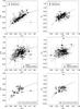 |
Fig. 3 (B − V) vs. (V − R) plots −left column − and (V − R) vs. (R − I) plots −right column − including the reddening line. Solar colors are indicated with the ⊙ symbol. Top panels: Plutinos and other resonants. Almost all non-Plutino resonants seem to lie on the reddening line in (B − V) vs. (V − R), but their stronger correlation value is within the error-bars of the correlations for other families. Middle panels: classical KBOs and all other KBOs, except Haumea family and retrogrades. In contrast to all other families, CKBOs do not exhibit a (B − V) vs. (V − R) correlation. The existence of many CKBOs far below the reddening line (in BVR), which indicates the presence of many concave visible spectra, suggests that they may exhibit absorption features in the visible that only detailed spectroscopic studies could verify. Bottom panels: binary or multiple KBOs. |
Classical KBOs, also known as classicals or CKBOs, are known for their color-inclination correlation, which is not clearly detected in any other family of KBOs (see Fig. 4 top). As for the case of other resonants, we removed the seven Haumea family objects from the classicals sample: 2003SQ317, 2003UZ117, 2005CB79, (024835) 1995SM55, (055636) 2002TX300, (120178) 2003OP32, and (145453) 2005RR43. When plotting B − R vs. orbital inclination i, we have three outliers with low B − R colors at very low inclination (see also Peixinho et al. 2008). Romanishin et al. (2010) analyzed a subfamily of classical objects with semi-major axes below the nominal location of the (3:2) resonance, calling them inner classicals. That subfamily presented a bimodal behavior of surface colors, unlike the rest of classical objects, and probably a distinct origin from the primordial protoplanetary disk. Although we did not use the same classification scheme, the outliers 1998WV24, and 2003YL179 belong to that group, and we decided to remove them from the analysis. There is, however, no similar indication why object 2002VD131 might be an outlier, but because of its extreme outlier behavior we chose to eliminate it as well. The final sample we analyzed has n = 117 classical objects (see Table 4).
5.6.1. Correlation of color vs. color of classical KBOs
CKBOs evidence neither (B − V) vs. (V − R) nor (V − R) vs. (R − I) correlations. And with their sample size, anything stronger than ρ ~ 0.43 should be detected at least at a 2.5σ level, although within the ρ error-bars we see that these correlations among KBOs∗, taken globally, increase when CKBOs are removed from the sample (see Table 4). The middle panel of Fig. 3 shows that this result seems clear. Interestingly, there are more CKBOs in the (B − V) vs. (V − R) plot far below the reddening line than for any other family. We return to this question in Sect. 5.9.2.
5.6.2. Correlation of color vs. orbital parameters of classical KBOs
The trend between the colors of classical objects and their orbital inclination was first reported by Tegler & Romanishin (2000). Explicit computations of a correlation were made later by Trujillo & Brown (2002) and Hainaut & Delsanti (2002).
This correlation was thought to be caused by some collisional evolution mechanism, known as collisional resurfacing (CR) − see Luu & Jewitt (1996)− which seemed highly dependent on the orbital inclination because of its link with a stronger or weaker collisional environment. Different parameters have been used to analyze it, such as collisional velocity, orbital excitation, ψ parameter, or simply orbital inclination. We analyzed each one of them, also including the Tissserand parameter relative to Neptune (TN).
Collisional velocity υc:
the mean square of a KBO encounter velocity with its circular analog, that is, a non-inclined circular orbit with heliocentric distance a, is given by  (5)
(5)
where e represents the orbital eccentricity, i stands for the orbital inclination relative to the ecliptic, and a for the semi-major axis. If a is measured in AU, then υK ≈ 29.8/![\hbox{$\!\sqrt{a}\;[\rm km\,s^{-1}]$}](/articles/aa/full_html/2015/05/aa25436-14/aa25436-14-eq230.png) . For simplicity, we call this υrms simply as collisional velocity υc.
. For simplicity, we call this υrms simply as collisional velocity υc.
Trujillo & Brown (2002) discussed the possible link between the color-inclination correlation and impact velocity but, given the lack of detailed modeling available at the time, they also discussed the possibility that the correlation might be a consequence of multiple subpopulations with different primordial colors and inclinations. Stern (2002) explored the link between KBO colors and their mean collisional velocities in more detail and also accounted for the gravitational effect of each object using  , where υesc is the KBO’s escape velocity, calculated assuming a bulk density ϱ = 1500kg m3 and a geometric albedo p = 0.04. Stern’s Spearman-rank correlations of (B − R) vs. υcoll and (B − V) vs. υcoll were ρBRυcoll = − 0.39(p = 0.005) and ρBVυcoll = − 0.44(p = 0.0005), respectively, for a total of n = 81 KBOs. Note that these correlation values are weaker than those reported by Trujillo & Brown for colors vs. inclination of classical KBOs also because Stern analyzed all families together. Nonetheless, these works seemed to confirm the existence of a physically meaningful correlation between KBO colors and their mean collision velocities, making a strong case for the CR scenario. From analyzing n = 50 CKBOs, Doressoundiram et al. (2002) reported ρBRυrms = − 0.49(p = 0.0004). Note that in spite of Stern’s care in also accounting for υesc to the collisional velocity from our sample we measure a median difference between υcoll and υrms of only 0.02km s-1, whereas the median υrms is 0.55km s-1. This is a very small difference given the uncertainty on the albedos and densities, and is the reason why υrms ≡ υc was used more often. It is noteworthy that Jewitt & Luu (2001), the proponents of the CR scenario, argued against it as the primary cause of color differences, since KBOs should then also exhibit large color variations with rotation, and observations indicated otherwise. Thébault & Doressoundiram (2003) and Thébault (2003) found additional problems with this scenario. Through a numerical analysis, they computed the kinetic energy KBOs would receive by collisions (hereafter Kcoll), considering several different swarms of impactors and also different KBO distributions. Results showed correlations between Kcoll and perihelion, but also that Kcoll correlated systematically much better with eccentricity than with inclination. Observationally, there was evidence for color vs. perihelion and color vs. inclination correlations but, to date, no relevant correlations between color and eccentricity has been found. Furthermore, from these simulations, Kcoll of Plutinos (3:2 resonants) was higher than the correlation of any other family, but observationally, their colors did not seem to differ. It is, nonetheless, true that this kind of numerical analysis has not been reanalyzed including the current understanding of the sculpting of the Kuiper belt through migration processes.
Orbital excitation ε:
Hainaut & Delsanti (2002) analyzed the color correlations with the object orbital excitation ε, defined as  (6)
(6)
This ε parameter is related with υrms (see Eq. (5)), which is another estimate of the KBO velocity with respect to its circular analog. Using Pearson’s correlation coefficient (rs) instead of Spearman’s, they obtained for (B − R) vs. ε of n = 13 CKBOs rs = − 0.77 (p = 0.0021P − valueisourestimate.), but no relevant values for any other families (rs< − 0.1), nor for KBOs and Centaurs taken together (rs = − 0.21, n = 34).
Öpik’s ψ:
Santos-Sanz et al. (2009) analyzed the color correlations with a ψ parameter, taken from the theory of Öpik (1976) of close encounters of a small body with a planet, given by  (7)
(7)
In our context, ψ relates with the average energy of the collisions experienced by a KBO. Again, the similarity between this parameter and the two previous ones is obvious. There is a subtle difference:  is an approximation for the KBO average encounter velocity with targets in circular orbits at the KBO instantaneous heliocentric distance on its elliptical orbit, that is, all local circular analogs. The two previous parameters consider only the impact with the global circular analog. Strangely, Santos-Sanz et al. (2009) reported for (B − R) vs. ψ of n = 64 CKBOs ρ = − 0.02. In our analysis we obtain
  (p< 10-6), as roughly expected given all the previous works.
Tisserand parameter TN:
the Tisserand parameter (Tisserand 1896), or invariant, has proven to be a useful tool in comet taxonomy (Kresák 1972; Levison 1996, and references therein). It is a dynamical quantity kept approximately constant during a close encounter interaction between a planet and a minor body − for instance, a KBO could have its orbital parameters changed by a close interaction with Neptune, and yet the Tisserand parameter value would not change, allowing us to keep track of the same object. Since KBOs are mostly under gravitational influence of Neptune, we compute it relative to this planet using  (8)where aN = 30.07AU is the semi-axis of Neptune and a, e, and i are the orbital parameters of the KBO. A minor body on a circular orbit, coplanar with Neptune, with a = aN would have TN = 3. A KBO, being a trans-Neptunian object, will have a>aN. If TN> 3, then it will not cross the orbit of Neptune, whereas if TN< 3 means, generally, a Neptune-crosser. Usage of TN in KBO taxonomy has been suggested by Elliot et al. (2005). Problems with the interpretation of TN values arise when high inclination values lead to a TN< 3, suggesting Neptune-crossing, even for impossible cases. For example, a KBO on a circular orbit with a = 37AU and i = 30° would have TN = 2.7 and it would not cross the orbit of Neptune. Note that TN parameter also relates with the relative encounter velocity between a KBO and Neptune:
  .
.
Regardless of the dynamical implications, Jewitt et al. (2007) reported for a total of n = 15 CKBOs (B − R) vs. TN and (U − B) vs. TN correlation values of  (p = 0.0014), and
  (p = 0.00004), respectively.
 |
Fig. 4 Top: (B − R) vs. orbital inclination plot of CKBOs and all KBOs with indication of Haumea family objects. The correlation for CKBOs alone is stronger than for all KBOs. The clustering of Haumea family objects had a strong effect on this correlation. Middle: Tisserand parameter relative to Neptune (TN) vs. orbital inclination as for the above. TN is very strongly correlated with i for CKBOs. Bottom: (B − R) vs. TN as for the above. Given the very strong link between TN and i, statistically one cannot know if only TN or i have a (potentially) physically meaningful relation with (B − R) but none dominates the other. |
Is there only one correlation?
CKBOs show moderate to strong correlations, all of similar magnitudes, both with i, υc, ε, ψ, and TN, and a moderate to weak correlation with q. The confidence level for the correlation between color and eccentricity does not reach the 2.5σ threshold after correcting for FDR, and no relevant correlation is detected between color and semi-major axis (see Table 2). From the correlations  ,
,  , and
, and  it is clear that both ψ, ε, and υc will be correlated with any other variable with the same strength. Consequently, analyzing for correlations between colors and collisional velocity υc, or orbital excitation ε, or the Öpik ψ is equivalent and, from a statistical point of view, there is no reason to chose one over the other. Hereafter, we chose to work with υc since it has been used more often in other works.
Spearman ρ correlation matrix between (B − R) and orbital parameters for n = 79 CKBOs.
Now, we consider the correlations between (B − R), TN, υc, i, and q more closely. Given the mutual dependence of most of these parameters, we have carried out a partial correlation analysis to assess whether one of these correlation is dominant and the others are only spurious effects with no physical relevance, but are present because of their dependence on the dominant one (see Sect. 3.1).
The partial correlations between (B − R), q, and i are  (9)
(9)
showing that the correlation between (B − R) colors and orbital inclination is still present and significant after removing the effect of the link between inclination and perihelion. Its strength, however, diminishes to a more moderate value. Perihelion is not a function of inclination, and the fact that q and i are correlated could be due to some dynamical evolution mechanism in the way the Kuiper belt was sculpted, or it may simply be the result of a sampling bias.
The partial correlations between (B − R), TN, and q are  (10)
(10)
showing that the correlation between (B − R) colors and Tisserand parameter is also still present and significant, although diminished to a more moderate value, after removing the effect of the link between TN and perihelion, analogously to the previous case.
The partial correlations between (B − R), TN, and i are  (11)
(11)
which shows that none remains after eliminating the effect of the other. This should not be seen as strange given that by definition TN is highly dependent on i, presenting a ρTNi = − 0.85, so it is very hard to separate one from the other.
The partial correlations between (B − R), i, and υc are  (12)
(12)
showing also that none remains after eliminating the effect of the other, even if the effect is stronger on inclination without the influence of collisional velocity than on υc without the effect of i. Analogously to the previous case, by definition the collisional velocity depends on inclination (ρυci = − 0.91), so it is hard to separate them.
Finally, the partial correlations between (B − R), TN, and υc are  (13)
(13)
indicating that none remains without the effect of the other variable, even if the case of ρ (B − R)υc.TN is rather close to 2.5σ.
To conclude, for CKBOs
-
it is statistically equivalent to use ψ, ε, or υc.
-
the correlation between (B − R) and perihelia may be simply an effect that arises because in the current sample of measured objects the perihelion is related with inclination, where inclination is the dominating variable. The same is true if we replace the variable inclination by the Tisserand parameter.
-
the correlations between (B − R) and both Tisserand parameter and inclination cannot be statistically separated from the close link between TN and i. None dominates the other (see Fig. 4).
-
although less clear than for the previous case, the correlation between (B − R) and collisional velocity cannot be statistically separated from the dependence of υc on inclination and on TN.
-
collisional velocity υc, Tisserand parameter TN, or orbital inclination i may be the true physically relevant variables linked with (B − R) surface colors.
-
given previous studies on the lack of evidence that surface colors are affected by υc, it is most likely that only either TN or i can be the variables that truly relate with colors − although causality cannot be assessed with this analysis –, and that dynamical history plays the central role.
It is interesting to note that CKBOs do not show evidence for a correlation between (B − V) vs. (V − R), which is present in almost all the other more undersampled families. We return to this matter in Sect. 5.9.1.
5.7. All KBOs∗
We have also analyzed the n = 322 KBOs∗ in our sample, that is all objects except Centaurs, Haumea family objects, and retrograde orbits. All color indexes correlate with each other, as expected from previous works. However, it is interesting to note that the color-inclination correlation for all KBOs, although weaker, is within the error-bars of the same correlation for CKBOs. This suggests that the colors of most non-CKBO families of KBOs are not totally uncorrelated with inclination, otherwise the correlation would be wiped out. The color-inclination correlation for n = 186 KBOs∗ removing the CKBOs is  , p = 0.000042, CL = 4.09 σ (better than 3σ after FDR correction). We must keep in mind that if the population’s ρ is − 0.5, to have only a 10% risk of failing to detect it at a 2.5σ level requires a sample of n = 55 objects, but if it is − 0.3, we need n = 156.
SDOs do have a sampling that should be enough to detect most correlations  | ± 0.5 | , but show
  (n = 54) with a p-value ≈0.50. Plutinos have a smaller sampling and show a
  (n = 45), the first correlation below the 2.5σ level after correcting for FDR. For non-Plutino resonants we have
  (n = 67), but below a 2σ level after correcting for FDR. These results indicate that it is unlikely that any non-CKBO family will have a yet-to-be detected color-inclination correlation stronger than − 0.5, but all may have a correlation of ~− 0.3 for which their sampling is too low to warrant detection. Clearly, the (B − R) vs. i trend is stronger among CKBOs, regardless of the current lower sampling of other families.
To verify this behavior, we have simulated 1000 samples with 79 (x,y) data-points correlated with ρ = − 0.50 (corresponding to our CKBOs) and 189 (x,y) data-points randomly generated, that is, with ρ ~ 0 (corresponding to the rest of our KBOs). The simulations show a distribution with  , which is not compatible with the observed , hence the weak color-inclination correlation seen among KBOs∗ is not simply a result of its stronger presence among CKBOs.
Weak correlations of ρ ~ ± 0.2 are detected between colors and perihelion and eccentricity. Although weak in magnitude and only accounting for ~5% of the color variability −ρ2 may be roughly interpreted as the proportion of the variability of Y that could be explained as a result of the variability of X− they are statistically significant, meaning that they are not a random effect.
5.8. Binary or multiple KBOs
Our sample has n = 48 binary or multiple objects, including Pluto and Haumea, and we have also analyzed the primaries of these systems as a group to see if they behave differently from the non-binaries.
Their color−color correlation does not show a different behavior from the previous cases. Their surface colors correlate both with TN, with υc, and i. A total of 26 out of these 48 objects are CKBOs, which are known to correlate with the aforementioned variables. Only n = 35 binary or multiple KBOs possess measured (B − R) colors, which means n = 14 CKBOs. Analyzing only the n = 20 non-CKBOs, also excluding Haumea, we obtain  , p = 0.027, CL = 2.21σ (without correcting for FDR). The result is not significant, and given the sample size, we have ρβ 2.5σ = − 0.76, which means that the subsampling is too small to confirm the existence of ρ(B − R)i ≈ − 0.50, like for CKBOs, or ρ(B − R)i ≈ − 0.30 like for non-CKBO KBOs as discussed above.
5.9. All∗ objects
As indicated in Sect. 2, we have removed from our global analysis objects belonging to the Haumea family and those with retrograde orbits. Our all∗ objects sample has n = 354 objects. The only relevant difference between the analysis of all∗ objects and that of KBOs∗ alone is the increase of the correlations between absolute magnitude HR and both q and a. These two cases may be simply interpreted as a bias. That is, fainter objects, which are most often also smaller, are hard to observe at high semi-major axes or high perihelia. When we include Centaurs in the sample, which are mostly small and faint, this becomes even more obvious. Nonetheless, it is a known fact that there are no large Centaurs, and this is not a bias.
5.9.1. Consecutive color correlations
Spearman ρ for consecutive colors.
Throughout all publications on the correlation between colors of Centaurs and KBOs, we see the tendency that with increasing wavelength of the region covered by the colors in question, the correlations tend to diminish. For example, in all works the correlations between (B − V) vs. (V − R) have been shown to be always stronger in magnitude than the correlations between (J − H) vs. (H − K). However, it is also a fact that the error-bars of visible colors are smaller than those of near-IR colors. Might this be the reason for the observed degradation of the correlation for increasing wavelength or not?
To answer this question, we have analyzed the relative median error-bar of each color normalized to the 6σ range of the corresponding color. For example, the 6 σ range of (B − V) color for all∗ is 1.036, the median error-bar is 0.08, therefore, after normalization, if (B − V) ranges from 0 to 1 the median error-bars would be 0.077. With this procedure we can use Eq. (4) and, with an assumption on the parent population ρ value, see the effect of the error-bars on the detectable ρ∗ (see Sect. 3.3)
Since the correlation of (B − V) vs. (V − R) usually is ~0.5 − 0.6, we assume, for simplicity, two cases: i) the parent population ρ is 0.7 and it should be 0.7 regardless of the spectral region we examine, ii) the same as the previous, but with ρ = 0.6. Table 3 summarizes the results. For each X vs. Y pair of colors we have their own sampling n, observed ρ, and normalized median error-bars σo. From Eq. (4) we compute the degraded ρDegraded ≡ ρ∗ for both 0.7 and 0.6, and from the sampling n we solve Eq. (2) to obtain the detectable ρ at a 2.5σ level accepting only a risk β = 0.1 of missing it, ρβ 2.5σ (see Sect. 3.2). Statistically ρ decreases with higher error-bars which are also typically associated with higher wavelengths but the variation is small. Observationally it decreases at a much faster rate. Therefore, we may conclude that, globally, the (B − V) vs. (V − R) correlation is stronger than the (V − R) vs. (R − I) one, and it is not an effect created by larger error-bars, that is, the color−color correlations do diminish with increasing wavelength. This result does not discard the possibility that this cannot be the case for some specific subgroups of objects, however.
Examining these correlations for each family in more detail, we may see a similar behavior for all of them except for CKBOs. The sampling of Plutinos, binary or multiple KBOs, Centaurs, and SDKBOs does not warrant detection of correlations weaker than ~0.6 at a β risk of 10%.
Since it is clear that the (V − R) vs. (R − I) correlation is indeed weaker than that of (B − V) vs. (V − R), it is not surprising that we do not detect it among SDOs, Plutinos, binary or multiple KBOs, or SDKBOs. For the latter we do not even detect the (B − V) vs. (V − R) correlation. For Centaurs, both are detected and show similar strengths. As a result of the low sampling, however, the correlation error-bars are too high to conclude that they are indeed similar, in contrast to what we have seen in other objects.
The most interesting case, however, are CKBOs, since these objects show neither (B − V) vs. (V − R) nor (V − R) vs. (R − I) correlations (see Sect. 5.6.1). The visible spectrophotometric behavior of CKBOs, or at least one type of CKBOs, is distinct from other KBOs. We discuss it below.
5.9.2. Peculiar convex spectrophotometric behaviors
Surface spectra of Centaurs and KBOs tend to be straight in the visible and flatten toward the near-IR JHK bands, most particularly when the visible slope is red, although the near-IR behavior tends to be more erratic. Figures 2 and 3 show that in (B − V) vs. (V − R) the objects tend to lie in the vicinity of the reddening line, meaning that they possess rather straight spectra in the BVR wavelength range (pictorially: − or ∕), or above it, meaning that they possess a slightly convex spectra in that same range (pictorially: ⌢). In the (V − R) vs. (R − I) plots we may see that objects are distributed above and below the reddening line. We have identified 11objects that fall far below the BVR reddening line: 2000CL104, 2002VT130, 2001RZ143, 1999JD132, 2001HY65, 2001HZ58, 1997RT5, 2000CL105, 2002VD1312 (all Classical KBOs), 2001KY76 (Plutino), and 1999RJ215 (SDO) − these are all mostly classical KBOs. Their normalized spectrophotometric reflectivity spectra are plotted in Fig. 5 along with the spectra resulting from the mean colors of all∗ objects (the error bars from the latter are the standard deviation of the color distribution and not the average error on each color). Spectra are normalized to 1 at the center of the V-band filter, and each one is shifted by 0.4 for clarity. The convex behavior these objects present in BVR might be a mere consequence of a concave (pictorially: ⌣) behavior in VRI, that is, the existence of an absorption band at ~6000 − 7000 Å. It is tempting to associate this behavior with aqueous altered minerals creating absorption features in this region, as once seen with spectroscopy on (38628) Huya and (47932) 2000GN171 by de Bergh et al. (2004), but the effect on visible colors is not expected to be very strong (see Barucci et al. 2008, for a review). The object 2001RZ143 does seem to be fully convex up to the I band, and we do not possess V − I colors of objects 2002VD131, 2000CL104, and 1999RJ215 to see if the spectral slope changes its convexity. Nonetheless, with the exception of 2001RZ143, the other 10 aforementioned objects seem good candidates to measure for the long-sought hydration features among Centaurs and KBOs or any other absorption feature in the visible spectrum.
 |
Fig. 5 Spectrophotometric reflectivity of 11 peculiar objects exhibiting a convex behavior at ~4500 − 6000 Å. Spectra are normalized to 1 at λ = 5454 Å and are consecutively shifted by 0.4 for clarity. This apparent convexity may be created by a concave behavior at ~6000 − 7000 Å, which suggests some absorption feature on their surfaces in this wavelength range. The spectrum resulting from the mean B − V, V − R, and V − I colors, and their standard deviations, for all∗ objects is shown in gray. |
5.10. Bimodal colors of small objects
Peixinho et al. (2012) found that both Centaurs and KBOs present the so-called bimodal (B − R) visible color behavior at a p-value = 0.001 (3.3σ) for absolute magnitudes  . In a somewhat different manner, Fraser & Brown (2012) found that all small objects (HR(α) ≳ 6) with perihelion q< 35 AU are bimodal, which will therefore include Centaurs. With this new dataset we have carried out the same analysis as Peixinho et al. (2012), obtaining a maximum of significance for the same bimodality for the n = 143 objects with
  , with a p-value = 0.0046 (2.8σ). Although the evidence for a bimodal behavior is very strong, we do not find a 3σ result with the new dataset (see Fig. 6).
Testing the n = 112 objects with perihelion q< 35 AU and  from the all∗ sample results in a p-value =0.126 (1.5σ), which means that there is no evidence for bimodality.
Interestingly, although the bimodality among Centaurs seems clear to the eye, when testing only for the n = 29 Centaurs in the sample we obtain a p-value = 0.018 (2.4σ).
 |
Fig. 6 (B − R) colors vs. HR(α) absolute magnitude (uncorrected for phase effects) for all objects in our database. Centaurs and KBOs are indicated with different symbols. Haumea family objects and the two retrograde objects are also highlighted. The |

6. Conclusions
We reanalyzed the correlations of BVRI-band visible colors for n = 354 Centaurs and KBOs. The (B − V), (V − R), (R − I), (B − R), (V − I), and (B − I) color indexes were carefully computed from all the available measurements in the literature, discarding color indexes computed from two bands taken more than two hours apart, and rejecting clear outliers from the averaging process. The complete sample consisted of n = 366 objects, but we removed from the analysis n = 2 objects with retrograde orbits and n = 10 Haumea family objects. Nonetheless, these objects were also plotted in our figures.
-
We used an algorithm for the Spearman-rank correlation − also known as Spearman-ρ− taking into account not only the data error-bars but also the error on the estimate due to the finite sampling and corrected the significance levels using the false-discovery rate (FDR) due to the large number of tests each sample was being subjected to.
-
We analyzed for the first time the risk β of missing any possible correlations as a result of our limited sampling and the sampling necessary to ensure detection at a chosen significance level.
-
With samples of n< 70 objects, assumed to be unbiased extractions of the parent population, we have a β> 10% risk of missing strong correlations, and if n< 90 medium strength (moderate) correlations may still be missed. When analyzing the traditional dynamical families, only classical KBOs, as a whole, do not require larger sampling to detect presumably relevant correlations. If one aims to study the subfamilies of hot classical, cold classical, inner classicals, or other, then larger samples are still needed. Centaurs are particularly undersampled and should be more than doubled. Plutinos and SDOs would benefit from a 50% sample increase. Other resonants, as a whole, are not undersampled, but like the Plutinos, each resonant family should be analyzed as a single group, and each one of them is largely undersampled. The sampling of the objects we grouped as scattered or detached KBOs would also need to be tripled. Note that the detection requirements for sample-size vs. correlation strength are general and would need to be applied to any possible subfamily or distinct classification one decides to study. However, the samples are assumed to be unbiased. Including possible sample biasing effects would require a more complex analysis.
-
We studied the degradation of a detectable correlation as a function of the data error-bars and concluded that after a certain correlation has been detected, it is pointless to increase the sampling while maintaining the same error-bars. Only by reducing the observational error-bars can a possibly stronger correlation be measured.
-
We showed that the location of the so-called reddening line in the color−color plots is quite sensitive to the central wavelengths of similar filters used on different telescopes. The effect is strong in the (B − V) vs. (V − R) plots, but weak in the (V − R) vs. (R − I) plots.
-
The correlation between (B − V) and (V − R) colors is stronger than the correlation between (V − R) and (R − I), regardless of the observational error-bars.
-
We analyzed the different parameters that have been used in the context of the color-inclination correlation of classical KBOs and the collisional resurfacing scenario using partial correlation tests. Statistically, it is equivalent to using the orbital excitation ε, Öpik’s ψ, or the collisional velocity υc. The detected color-perihelion correlation is most likely physically irrelevant and an effect of the strong relation between perihelion q and inclination i among CKBOs. Both orbital inclination i and Tisserand parameter relative to Neptune TN are the most likely physically relevant parameters related with the color variation of CKBOs, therefore the relation is probably related to dynamical history alone. Statistically, the collisional velocity cannot be separated from its dependence on inclination i or TN. Without the Haumea family, the color-inclination correlation of CKBOs is no longer strong, but moderate (ρ ~ 0.5).
-
Although weaker than for CKBOs, a color-inclination correlation must still exist among the non-classical KBOs.
-
Classical KBOs are the only family that show neither (B − V) vs. (V − R) nor (V − R) vs. (R − I) correlation.
-
We identified ten objects, only two of which are not CKBOs, that exhibit a convex spectral behavior from their (B − V) and (V − R) colors and a concave behavior from their (V − R) and (R − I) colors, suggesting an absorption band or feature at ~6000 − 7000 Å, which renders them good candidates for detailed spectroscopic studies.
-
We detected evidence for the (B − R) color bimodality for objects with absolute magnitude
at a 2.8σ level (p-value = 0.0046) − see Peixinho et al. (2012). Paradoxically, the evidence for bimodality among Centaurs reaches only 2.4σ− see Peixinho et al. (2003) –, and we find no evidence for bimodality of objects with perihelion q< 35 AU and − see Fraser & Brown (2012).
We must stress that we analyzed the correlations and sampling requirements of the traditional dynamical families of KBOs and Centaurs as defined in Sect. 2, with the aim to characterize each of them, and with the underlying statistical assumption that each sample is or will be unbiased. The physical and/or chemical relevance of the dynamical classification system used was not discussed. Using distinct classification systems, subsystems, or groupings should lead to distinct correlations as well as to distinct sampling considerations, and such works are to be encouraged.
A similar study, extended to the near-IR colors, is under preparation.
ftp://ftp.lowell.edu/pub/elgb/astorb.dat.gz, with epoch 20120420.
Acknowledgments
We thank the anonymous referee for the comments that helped to improve this manuscript. We thank Audrey Thirouin for her LaTeX “magic”. N.P. acknowledges funding by the Gemini-Conicyt Fund, allocated to the project No. 32120036.
References
- Alvarez-Candal, A., Barucci, M. A., Merlin, F., et al. 2010, A&A, 511, A35 [NASA ADS] [CrossRef] [EDP Sciences] [Google Scholar]
- Barucci, M. A., Doressoundiram, A., Tholen, D., Fulchignoni, M., & Lazzarin, M. 1999, Icarus, 142, 476 [NASA ADS] [CrossRef] [Google Scholar]
- Barucci, M. A., Romon, J., Doressoundiram, A., & Tholen, D. J. 2000, AJ, 120, 496 [NASA ADS] [CrossRef] [Google Scholar]
- Barucci, M. A., Boehnhardt, H., Dotto, E., et al. 2002, A&A, 392, 335 [NASA ADS] [CrossRef] [EDP Sciences] [Google Scholar]
- Barucci, M. A., Belskaya, I. N., Fulchignoni, M., & Birlan, M. 2005, AJ, 130, 1291 [NASA ADS] [CrossRef] [Google Scholar]
- Barucci, M. A., Brown, M. E., Emery, J. P., & Merlin, F. 2008, Composition and Surface Properties of Transneptunian Objects and Centaurs, eds. M. A. Barucci, H. Boehnhardt, D. P. Cruikshank, A. Morbidelli, & R. Dotson, 143 [Google Scholar]
- Batygin, K., Brown, M. E., & Fraser, W. C. 2011, ApJ, 738, 13 [NASA ADS] [CrossRef] [Google Scholar]
- Bauer, J. M., Meech, K. J., Fernández, Y. R., et al. 2003, Icarus, 166, 195 [NASA ADS] [CrossRef] [Google Scholar]
- Benecchi, S. D., Noll, K. S., Grundy, W. M., et al. 2009, Icarus, 200, 292 [NASA ADS] [CrossRef] [Google Scholar]
- Benecchi, S. D., Noll, K. S., Stephens, D. C., Grundy, W. M., & Rawlins, J. 2011, Icarus, 213, 693 [NASA ADS] [CrossRef] [Google Scholar]
- Benjamini, Y., & Hochberg, Y. 1995, J. Roy. Statist. Soc. Ser. B (Methodological), 57, 289 [Google Scholar]
- Boehnhardt, H., Tozzi, G. P., Birkle, K., et al. 2001, A&A, 378, 653 [NASA ADS] [CrossRef] [EDP Sciences] [Google Scholar]
- Boehnhardt, H., Delsanti, A., Barucci, A., et al. 2002, A&A, 395, 297 [NASA ADS] [CrossRef] [EDP Sciences] [Google Scholar]
- Boehnhardt, H., Bagnulo, S., Muinonen, K., et al. 2004, A&A, 415, L21 [NASA ADS] [CrossRef] [EDP Sciences] [Google Scholar]
- Bonett, D. G., & Wright, T. A. 2000, Psychometrika, 65, 23 [CrossRef] [Google Scholar]
- Bonferroni, C. E. 1935, Il calcolo delle assicurazioni su gruppi di teste, ed. Rome, Italy, 13 [Google Scholar]
- Brown, M. E., Barkume, K. M., Ragozzine, D., & Schaller, E. L. 2007, Nature, 446, 294 [NASA ADS] [CrossRef] [PubMed] [Google Scholar]
- Brown, M. E., Schaller, E. L., & Fraser, W. C. 2011, ApJ, 739, L60 [NASA ADS] [CrossRef] [Google Scholar]
- Dalle Ore, C. M., Dal le Ore, L. V., Roush, T. L., et al. 2013, Icarus, 222, 307 [NASA ADS] [CrossRef] [Google Scholar]
- de Bergh, C., Boehnhardt, H., Barucci, M. A., et al. 2004, A&A, 416, 791 [NASA ADS] [CrossRef] [EDP Sciences] [Google Scholar]
- de Bergh, C., Delsanti, A., Tozzi, G. P., et al. 2005, A&A, 437, 1115 [NASA ADS] [CrossRef] [EDP Sciences] [Google Scholar]
- Delsanti, A. C., Boehnhardt, H., Barrera, L., et al. 2001, A&A, 380, 347 [NASA ADS] [CrossRef] [EDP Sciences] [Google Scholar]
- Delsanti, A., Hainaut, O., Jourdeuil, E., et al. 2004, A&A, 417, 1145 [NASA ADS] [CrossRef] [EDP Sciences] [Google Scholar]
- Delsanti, A., Peixinho, N., Boehnhardt, H., et al. 2006, AJ, 131, 1851 [NASA ADS] [CrossRef] [Google Scholar]
- DeMeo, F. E., Fornasier, S., Barucci, M. A., et al. 2009, A&A, 493, 283 [NASA ADS] [CrossRef] [EDP Sciences] [Google Scholar]
- DeMeo, F. E., Barucci, M. A., Merlin, F., et al. 2010, A&A, 521, A35 [NASA ADS] [CrossRef] [EDP Sciences] [Google Scholar]
- Doressoundiram, A., Barucci, M. A., Romon, J., & Veillet, C. 2001, Icarus, 154, 277 [NASA ADS] [CrossRef] [Google Scholar]
- Doressoundiram, A., Peixinho, N., de Bergh, C., et al. 2002, AJ, 124, 2279 [NASA ADS] [CrossRef] [Google Scholar]
- Doressoundiram, A., Barucci, M. A., Tozzi, G. P., et al. 2005a, Planet. Space Sci., 53, 1501 [Google Scholar]
- Doressoundiram, A., Peixinho, N., Doucet, C., et al. 2005b, Icarus, 174, 90 [NASA ADS] [CrossRef] [Google Scholar]
- Doressoundiram, A., Peixinho, N., Moullet, A., et al. 2007, AJ, 134, 2186 [NASA ADS] [CrossRef] [Google Scholar]
- Doressoundiram, A., Boehnhardt, H., Tegler, S. C., & Trujillo, C. 2008, Color Properties and Trends of the Transneptunian Objects, eds. M. A. Barucci, H. Boehnhardt, D. P. Cruikshank, A. Morbidelli, & R. Dotson, 91 [Google Scholar]
- Dotto, E., Barucci, M. A., Boehnhardt, H., et al. 2003, Icarus, 162, 408 [NASA ADS] [CrossRef] [Google Scholar]
- Edgeworth, K. E. 1943, J. British Astron. Assoc., 53, 181 [Google Scholar]
- Edgeworth, K. E. 1949, MNRAS, 109, 600 [NASA ADS] [CrossRef] [Google Scholar]
- Efron, B., & Tibshirani, R. J. 1993, An Introduction to the Bootstrap (Chapman & Hall/CRC) [Google Scholar]
- Elliot, J. L., Kern, S. D., Clancy, K. B., et al. 2005, AJ, 129, 1117 [NASA ADS] [CrossRef] [Google Scholar]
- Emel’yanenko, V. V., Asher, D. J., & Bailey, M. E. 2013, Earth Moon and Planets, 110, 105 [NASA ADS] [CrossRef] [Google Scholar]
- Fernandez, J. A. 1980, MNRAS, 192, 481 [NASA ADS] [CrossRef] [Google Scholar]
- Ferrin, I., Rabinowitz, D., Schaefer, B., et al. 2001, ApJ, 548, L243 [Google Scholar]
- Fisher, R. A. 1915, Biometrika, 10, 507 [Google Scholar]
- Fornasier, S., Doressoundiram, A., Tozzi, G. P., et al. 2004, A&A, 421, 353 [NASA ADS] [CrossRef] [EDP Sciences] [Google Scholar]
- Fouchard, M., Rickman, H., Froeschlé, C., & Valsecchi, G. B. 2014, Icarus, 231, 99 [NASA ADS] [CrossRef] [Google Scholar]
- Fraser, W. C., & Brown, M. E. 2012, ApJ, 749, 33 [NASA ADS] [CrossRef] [Google Scholar]
- Gil-Hutton, R. 2002, Planet. Space Sci., 50, 57 [NASA ADS] [CrossRef] [Google Scholar]
- Gil-Hutton, R., & Licandro, J. 2001, Icarus, 152, 246 [NASA ADS] [CrossRef] [Google Scholar]
- Gladman, B., Marsden, B. G., & Vanlaerhoven, C. 2008, Nomenclature in the Outer Solar System, eds. M. A. Barucci, H., Boehnhardt, D. P. Cruikshank, A. Morbidelli, & R. Dotson (Tucson: University of Arizona Press), 592, 43 [Google Scholar]
- Gomes, R. S. 2003, Icarus, 161, 404 [Google Scholar]
- Green, S. F., McBride, N., O’Ceallaigh, D. P., et al. 1997, MNRAS, 290, 186 [NASA ADS] [CrossRef] [Google Scholar]
- Gulbis, A. A. S., Elliot, J. L., & Kane, J. F. 2006, Icarus, 183, 168 [NASA ADS] [CrossRef] [Google Scholar]
- Hainaut, O. R., & Delsanti, A. C. 2002, A&A, 389, 641 [NASA ADS] [CrossRef] [EDP Sciences] [Google Scholar]
- Hainaut, O. R., Delahodde, C. E., Boehnhardt, H., et al. 2000, A&A, 356, 1076 [NASA ADS] [Google Scholar]
- Hainaut, O. R., Boehnhardt, H., & Protopapa, S. 2012, A&A, 546, A115 [NASA ADS] [CrossRef] [EDP Sciences] [Google Scholar]
- Horner, J., Evans, N. W., & Bailey, M. E. 2004, MNRAS, 354, 798 [NASA ADS] [CrossRef] [Google Scholar]
- Jewitt, D., & Luu, J. 1993, Nature, 362, 730 [NASA ADS] [CrossRef] [Google Scholar]
- Jewitt, D., & Luu, J. 1998, AJ, 115, 1667 [NASA ADS] [CrossRef] [Google Scholar]
- Jewitt, D. C., & Luu, J. X. 2001, AJ, 122, 2099 [NASA ADS] [CrossRef] [Google Scholar]
- Jewitt, D., Peixinho, N., & Hsieh, H. H. 2007, AJ, 134, 2046 [NASA ADS] [CrossRef] [Google Scholar]
- Kaňuchová, Z., Brunetto, R., Melita, M., & Strazzulla, G. 2012, Icarus, 221, 12 [NASA ADS] [CrossRef] [Google Scholar]
- Kavelaars, J., Jones, L., Gladman, B., Parker, J. W., & Petit, J.-M. 2008, The Orbital and Spatial Distribution of the Kuiper belt, Asteroids, Comets, Meteors 2008 held July 14–18, 2008 in Baltimore, Maryland, LPI Contribution No. 1405 eds. M. A. Barucci, H. Boehnhardt, D. P. Cruikshank, et al., 59 [Google Scholar]
- Kendall, M. G., Kendall, S. F. H., & Smith, B. B. 1939, Biometrika, 30, 251 [Google Scholar]
- Kresák, L. 1972, in The Motion, Evolution of Orbits, and Origin of Comets, eds. G. A. Chebotarev, E. I. Kazimirchak-Polonskaia, & B. G. Marsden, IAU Symp., 45, 503 [Google Scholar]
- Kuiper, G. P. 1951, in Proc. topical Symp., commemorating the 50th anniversary of the Yerkes Observatory and half a century of progress in astrophysics, ed. J. Hynek (New York: McGraw-Hill), 357 [Google Scholar]
- Lacerda, P., Fornasier, S., Lellouch, E., et al. 2014, ApJ, 793, L2 [NASA ADS] [CrossRef] [Google Scholar]
- Lazzaro, D., Florczak, M. A., Angeli, C. A., et al. 1997, Planet. Space Sci., 45, 1607 [NASA ADS] [CrossRef] [Google Scholar]
- Leonard, F. C. 1930, Leaflet of the Astronical Society of the Pacific, 1, 121 [Google Scholar]
- Levenberg, K. 1944, Quarterly J. Appl. Math., II, 164 [Google Scholar]
- Levison, H. F. 1996, in Completing the Inventory of the Solar System, ASP Conf. Ser., 107, 173 [NASA ADS] [Google Scholar]
- Levison, H. F., & Duncan, M. J. 1997, Icarus, 127, 13 [Google Scholar]
- Levison, H. F., Morbidelli, A., Tsiganis, K., Nesvorný, D., & Gomes, R. 2011, AJ, 142, 152 [NASA ADS] [CrossRef] [Google Scholar]
- Luu, J., & Jewitt, D. 1996, AJ, 112, 2310 [NASA ADS] [CrossRef] [Google Scholar]
- Lykawka, P. S., & Mukai, T. 2007, Icarus, 189, 213 [NASA ADS] [CrossRef] [Google Scholar]
- Macklin, J. T. 1982, MNRAS, 199, 1119 [NASA ADS] [Google Scholar]
- Marquardt, D. W. 1963, SIAM J. Appl. Math., 11, 431 [Google Scholar]
- Miller, R. G. 1981, Simultaneous Statistical Inference (New York: Springer, 2nd edn.), 299 [Google Scholar]
- Modarres, R. 1996, Statistics and Computing, 6, 139 [CrossRef] [Google Scholar]
- Öpik, E. J. 1976, Interplanetary encounters: close-range gravitational interactions (Elsevier Science Ltd), Amsterdam: 2, 160 [Google Scholar]
- Peixinho, N., Lacerda, P., Ortiz, J. L., et al. 2001, A&A, 371, 753 [NASA ADS] [CrossRef] [EDP Sciences] [Google Scholar]
- Peixinho, N., Doressoundiram, A., Delsanti, A., et al. 2003, A&A, 410, L29 [NASA ADS] [CrossRef] [EDP Sciences] [Google Scholar]
- Peixinho, N., Boehnhardt, H., Belskaya, I., et al. 2004, Icarus, 170, 153 [NASA ADS] [CrossRef] [Google Scholar]
- Peixinho, N., Lacerda, P., & Jewitt, D. 2008, AJ, 136, 1837 [NASA ADS] [CrossRef] [Google Scholar]
- Peixinho, N., Delsanti, A., Guilbert-Lepoutre, A., Gafeira, R., & Lacerda, P. 2012, A&A, 546, A86 [NASA ADS] [CrossRef] [EDP Sciences] [Google Scholar]
- Perna, D., Barucci, M. A., Fornasier, S., et al. 2010, A&A, 510, A53 [NASA ADS] [CrossRef] [EDP Sciences] [Google Scholar]
- Petit, J.-M., Kavelaars, J. J., Gladman, B. J., et al. 2011, AJ, 142, 131 [NASA ADS] [CrossRef] [Google Scholar]
- Rabinowitz, D. L., Barkume, K., Brown, M. E., et al. 2006, ApJ, 639, 1238 [NASA ADS] [CrossRef] [Google Scholar]
- Rabinowitz, D. L., Schaefer, B. E., & Tourtellotte, S. W. 2007, AJ, 133, 26 [NASA ADS] [CrossRef] [Google Scholar]
- Rabinowitz, D. L., Schaefer, B. E., Schaefer, M., & Tourtellotte, S. W. 2008, AJ, 136, 1502 [NASA ADS] [CrossRef] [Google Scholar]
- Ramírez, I., Michel, R., Sefako, R., et al. 2012, ApJ, 752, 5 [NASA ADS] [CrossRef] [Google Scholar]
- Romanishin, W., Tegler, S. C., Levine, J., & Butler, N. 1997, AJ, 113, 1893 [NASA ADS] [CrossRef] [Google Scholar]
- Romanishin, W., Tegler, S. C., & Consolmagno, G. J. 2010, AJ, 140, 29 [NASA ADS] [CrossRef] [Google Scholar]
- Romon-Martin, J., Barucci, M. A., de Bergh, C., et al. 2002, Icarus, 160, 59 [NASA ADS] [CrossRef] [Google Scholar]
- Romon-Martin, J., Delahodde, C., Barucci, M. A., de Bergh, C., & Peixinho, N. 2003, A&A, 400, 369 [NASA ADS] [CrossRef] [EDP Sciences] [Google Scholar]
- Santos-Sanz, P., Ortiz, J. L., Barrera, L., & Boehnhardt, H. 2009, A&A, 494, 693 [NASA ADS] [CrossRef] [EDP Sciences] [Google Scholar]
- Santos-Sanz, P., Lellouch, E., Fornasier, S., et al. 2012, A&A, 541, A92 [NASA ADS] [CrossRef] [EDP Sciences] [Google Scholar]
- Sheppard, S. S. 2010, AJ, 139, 1394 [NASA ADS] [CrossRef] [PubMed] [Google Scholar]
- Sheppard, S. S. 2012, AJ, 144, 169 [NASA ADS] [CrossRef] [Google Scholar]
- Snodgrass, C., Carry, B., Dumas, C., & Hainaut, O. 2010, A&A, 511, A72 [NASA ADS] [CrossRef] [EDP Sciences] [Google Scholar]
- Spearman, C. 1904, Am. J. Psychol., 57, 72 [CrossRef] [Google Scholar]
- Stern, S. A. 2002, AJ, 124, 2297 [NASA ADS] [CrossRef] [Google Scholar]
- Tegler, S. C., & Romanishin, W. 1997, Icarus, 126, 212 [NASA ADS] [CrossRef] [Google Scholar]
- Tegler, S. C., & Romanishin, W. 1998, Nature, 392, 49 [NASA ADS] [CrossRef] [Google Scholar]
- Tegler, S. C., & Romanishin, W. 2000, Nature, 407, 979 [NASA ADS] [CrossRef] [PubMed] [Google Scholar]
- Tegler, S. C., & Romanishin, W. 2003, Icarus, 161, 181 [NASA ADS] [CrossRef] [Google Scholar]
- Tegler, S. C., Romanishin, W., & Consolmagno, G. J. 2003, ApJ, 599, L49 [NASA ADS] [CrossRef] [Google Scholar]
- Thébault, P. 2003, Earth Moon Planet, 92, 233 [Google Scholar]
- Thébault, P., & Doressoundiram, A. 2003, Icarus, 162, 27 [NASA ADS] [CrossRef] [Google Scholar]
- Tisserand, F. 1896, Traité de Mécanique Céleste (Tome IV) (Gauthier-Villars, Paris) [Google Scholar]
- Trujillo, C. A., & Brown, M. E. 2002, ApJ, 566, L125 [NASA ADS] [CrossRef] [Google Scholar]
All Tables
Spearman ρ correlation matrix between (B − R) and orbital parameters for n = 79 CKBOs.
All Figures
|
Fig. 1 (B − V) vs. (V − R)−top − and (V − R) vs. (R − I)−bottom− reddening lines obtained with the most frequently used sets of BVRI filters in our database and the computed average reddening line. For the (B − V) vs. (V − R) case different filters have a strong effect on the location of the reddening line. For the (V − R) vs. (R − I) case the effect is almost negligible. |
| In the text | |
|
Fig. 2 (B − V) vs. (V − R) plots −left column − and (V − R) vs. (R − I) plots −right column − including the reddening line. Solar colors are indicated with the ⊙ symbol. Top panels: all objects, Haumea family objects, and retrograde objects. Middle panels: Centaurs. Bottom panels: scattered disk objects (SDOs), and scattered or detached Kuiper belt objects (SDKBOs). The stronger correlation between (B − V) and (V − R) colors than between (V − R) and (R − I) is clear. Apart from the solar-like colors of Haumea family objects and the two color groups of Centaurs in the (B − V) vs. (V − R) there is no apparent relevant difference between the color distribution of each family of objects. |
| In the text | |
|
Fig. 3 (B − V) vs. (V − R) plots −left column − and (V − R) vs. (R − I) plots −right column − including the reddening line. Solar colors are indicated with the ⊙ symbol. Top panels: Plutinos and other resonants. Almost all non-Plutino resonants seem to lie on the reddening line in (B − V) vs. (V − R), but their stronger correlation value is within the error-bars of the correlations for other families. Middle panels: classical KBOs and all other KBOs, except Haumea family and retrogrades. In contrast to all other families, CKBOs do not exhibit a (B − V) vs. (V − R) correlation. The existence of many CKBOs far below the reddening line (in BVR), which indicates the presence of many concave visible spectra, suggests that they may exhibit absorption features in the visible that only detailed spectroscopic studies could verify. Bottom panels: binary or multiple KBOs. |
| In the text | |
|
Fig. 4 Top: (B − R) vs. orbital inclination plot of CKBOs and all KBOs with indication of Haumea family objects. The correlation for CKBOs alone is stronger than for all KBOs. The clustering of Haumea family objects had a strong effect on this correlation. Middle: Tisserand parameter relative to Neptune (TN) vs. orbital inclination as for the above. TN is very strongly correlated with i for CKBOs. Bottom: (B − R) vs. TN as for the above. Given the very strong link between TN and i, statistically one cannot know if only TN or i have a (potentially) physically meaningful relation with (B − R) but none dominates the other. |
| In the text | |
|
Fig. 5 Spectrophotometric reflectivity of 11 peculiar objects exhibiting a convex behavior at ~4500 − 6000 Å. Spectra are normalized to 1 at λ = 5454 Å and are consecutively shifted by 0.4 for clarity. This apparent convexity may be created by a concave behavior at ~6000 − 7000 Å, which suggests some absorption feature on their surfaces in this wavelength range. The spectrum resulting from the mean B − V, V − R, and V − I colors, and their standard deviations, for all∗ objects is shown in gray. |
| In the text | |
|
Fig. 6 (B − R) colors vs. HR(α) absolute magnitude (uncorrected for phase effects) for all objects in our database. Centaurs and KBOs are indicated with different symbols. Haumea family objects and the two retrograde objects are also highlighted. The |
| In the text | |
Current usage metrics show cumulative count of Article Views (full-text article views including HTML views, PDF and ePub downloads, according to the available data) and Abstracts Views on Vision4Press platform.
Data correspond to usage on the plateform after 2015. The current usage metrics is available 48-96 hours after online publication and is updated daily on week days.
Initial download of the metrics may take a while.