| Issue |
A&A
Volume 577, May 2015
|
|
|---|---|---|
| Article Number | A38 | |
| Number of page(s) | 9 | |
| Section | Extragalactic astronomy | |
| DOI | https://doi.org/10.1051/0004-6361/201425401 | |
| Published online | 28 April 2015 | |
Anatomy of the AGN in NGC 5548
III. The high-energy view with NuSTAR and INTEGRAL
1
Univ. Grenoble Alpes, IPAG,
38000
Grenoble,
France
e-mail:
This email address is being protected from spambots. You need JavaScript enabled to view it.
2
CNRS, IPAG, 38000
Grenoble,
France
3
Dipartimento di Matematica e Fisica, Università degli Studi Roma
Tre, via della Vasca Navale
84, 00146
Roma,
Italy
4
Department of Astronomy, University of Geneva,
16 Ch. d’Ecogia, 1290
Versoix,
Switzerland
5
INAF-IASF Bologna, via Gobetti 101, 40129
Bologna,
Italy
6
SRON Netherlands Institute for Space Research,
Sorbonnelaan 2, 3584 CA
Utrecht, The
Netherlands
7
Cahill Center for Astronomy and Astrophysics, California Institute
of Technology, Pasadena, CA
91125,
USA
8
Jet Propulsion Laboratory, 4800 Oak Grove Dr., Pasadena, CA
91109,
USA
9
Max-Planck-Institut für extraterrestrische Physik,
Giessenbachstrasse,
85748
Garching,
Germany
10
Space Telescope Science Institute, 3700 San Martin Drive, Baltimore, MD
21218,
USA
11
Department of Physics and Astronomy, The Johns Hopkins
University, Baltimore, MD
21218,
USA
12
Mullard Space Science Laboratory, University College
London, Holmbury St. Mary,
Dorking, Surrey,
RH5 6NT,
UK
13
Department of Astronomy, The Ohio State University,
140 W 18th Avenue, Columbus, OH
43210,
USA
14
Center for Cosmology & AstroParticle Physics, The Ohio
State University, 191 West Woodruff
Avenue, Columbus,
OH
43210,
USA
15
Instituto de Astronomia, Universidad Católica del
Norte, Avenida Angamos 0610,
Casilla 1280, Antofagasta, Chile
16
Department of Physics, University of Oxford,
Keble Road, Oxford, OX1
3RH, UK
Received: 25 November 2014
Accepted: 12 January 2015
Abstract
We describe the analysis of the seven broad-band X-ray continuum observations of the archetypal Seyfert 1 galaxy NGC 5548 that were obtained with XMM-Newton or Chandra, simultaneously with high-energy (>10 keV) observations with NuSTAR and INTEGRAL. These data were obtained as part of a multiwavelength campaign undertaken from the summer of 2013 till early 2014. We find evidence of a high-energy cut-off in at least one observation, which we attribute to thermal Comptonization, and a constant reflected component that is likely due to neutral material at least a few light months away from the continuum source. We confirm the presence of strong, partial covering X-ray absorption as the explanation for the sharp decrease in flux through the soft X-ray band. The obscurers appear to be variable in column density and covering fraction on time scales as short as weeks. A fit of the average spectrum over the range 0.3–400 keV with a realistic Comptonization model indicates the presence of a hot corona with a temperature of 40+40-10 keV and an optical depth of 2.7+0.7-1.2 if a spherical geometry is assumed.
Key words: galaxies: active / galaxies: Seyfert / X-rays: galaxies
© ESO, 2015
1. Introduction
Logs of the simultaneous XMM-Newton, NuSTAR, and/or INTEGRAL observations of NGC 5548 during our campaign.
The high-energy spectrum of active galactic nuclei (AGNs) is typically dominated by a primary power law component, which is generally believed to originate in a hot plasma, the so-called corona, localized in the inner part of the accretion flow (Reis & Miller 2013). The presence of a high-energy cut-off around ~100 keV has been observed in several sources (see, e.g., Perola et al. 2002; Malizia et al. 2014; Brenneman et al. 2014; Marinucci et al. 2014; Ballantyne et al. 2014) and is commonly interpreted as the signature of thermal Comptonization. Namely, the optical/UV photons from the accretion disk are upscattered by the hot electrons of the corona up to X-ray energies (see, e.g., Haardt & Maraschi 1991; Haardt et al. 1994, 1997). This primary emission can be modified by different processes, such as absorption from surrounding gas and Compton reflection from the disk itself or more distant material. Moreover, the spectra of many AGNs rise smoothly below 1–2 keV above the extrapolated high-energy power law (see, e.g., Bianchi et al. 2009). The nature of this so-called soft excess is still under debate (see, e.g., Done et al. 2012).
The geometrical and physical properties of the different structures leading to the different spectral components are still poorly known. First and foremost, a more complete understanding of the high-energy emission of AGNs requires disentangling the spectral properties of each component and constraining their characteristic parameters. For this goal, the availability of multiple broad-band observations with a high signal-to-noise ratio is essential. Using the data from a previous long multiwavelength campaign on Mrk 509 (Kaastra et al. 2011), Petrucci et al. (2013) made a detailed study of the high-energy spectrum of that AGN. In that case, the simultaneous data covering the range from optical/UV to gamma-ray energies made it possible to test Comptonization models in full detail and provide a physically motivated picture of the inner regions of the source. The hard X-ray continuum was well fitted by a Comptonized spectrum produced by a hot, optically thin corona with kTe ~ 100 keV and τ ~ 0.5, probably localized in the very inner part of the accretion flow (Petrucci et al. 2013). Mehdipour et al. (2011), studying the optical to X-ray variability, found a correlation between the optical/UV and soft (<0.5 keV) X-ray flux, but no correlation between the optical/UV and hard (>3 keV) X-ray flux. This result was interpreted as indicating the presence of a second, “warm” corona with kTe ~ 1 keV and τ ~ 15, responsible for the soft excess as well as the optical/UV emission (Mehdipour et al. 2011; Petrucci et al. 2013).
In the present paper, we discuss results based on a multiwavelength monitoring program on the AGN NGC 5548, an X-ray bright Seyfert 1 galaxy, hosting a supermassive black hole of 3.9 × 10⁷ solar masses (Pancoast et al. 2014) and lying at a redshift of z = 0.017175 (de Vaucouleurs et al. 1991,as given in the NASA/IPAC Extragalactic Database). The source historically presented a flux variability typical of an unobscured AGN of that black hole mass (Ponti et al. 2012). High spectral resolution X-ray and UV observations of this source have previously shown a typical ionized outflow, seen as the “warm absorber” through narrow lines absorbing the UV and soft X-ray emission from the core (Crenshaw et al. 2003; Steenbrugge et al. 2005).
The multiwavelength campaign was conducted from May 2013 to February 2014, involving observations with the XMM-Newton, HST, Swift, NuSTAR, INTEGRAL and Chandra satellites (Kaastra et al. 2014, hereafter K14). During the campaign, the nucleus was found to be obscured by a long-lasting and clumpy stream of ionized gas never seen before in this source. This heavy absorption manifests itself as a 90% decrease of the soft X-ray continuum emission, associated with deep and broad UV absorption troughs. The obscuring material has a distance of only a few light days from the nucleus, and it is outflowing with a velocity up to five times faster than those observed in the warm absorber (K14). Given its properties, this new obscuring stream likely arises in the accretion disk.
This work is part of a series of papers focusing on different aspects of the campaign. Here we concentrate on the broad band (0.3–400 keV) X-ray emission, focusing on the observations featuring high-energy (>10 keV) data provided by NuSTAR and INTEGRAL.
The paper is organized as follows. In Sect. 2, we describe the observations and data reduction. In Sect. 3 we present the analysis of the hard (>5 keV) X-ray and total (0.3–400 keV) X-ray spectrum, fitted with both a phenomenological and a realistic Comptonization model. In Sect. 4, we discuss the results and summarize our conclusions.
2. Observations and data reduction
The multi-satellite campaign was led by XMM-Newton, which observed NGC 5548 twelve times during 40 days in June and July 2013, plus once in December and once in February 2014. For the full description of the program, see K14 and Mehdipour et al. (2015). During the campaign, NuSTAR (Harrison et al. 2013) and INTEGRAL (Winkler et al. 2003) regularly observed the source simultaneously with XMM-Newton. A simultaneous Chandra/NuSTAR observation was also performed in September 2013. The log of the data sets analysed in this paper is reported in Table 1, with their observation ID, their start date, and net exposure time. The latest XMM-Newton observation is dated February 4, and the corresponding spectrum has been analysed jointly with an average spectrum obtained from three INTEGRAL exposures obtained in January and February, which show no significant variations.
In all the XMM-Newton observations, the EPIC instruments were operating in the Small-Window mode with the thin-filter applied. For our analysis, we used the EPIC-pn data only. The data were processed using the XMM-Newton Science Analysis System (sas v13). The spectra were grouped such that each spectral bin contains at least 20 counts. Starting in 2013, a gain problem with the pn data appeared, causing a shift of about 50 eV near the Fe-K complex (see the detailed discussion in Cappi et al., in prep.). In the present paper this shift was corrected for by leaving the redshift free to vary in our models. Moreover, this small offset yields poor fits near the energy of the gold M-edge of the telescope mirror, and for this reason the interval between 2.0 and 2.5 keV was omitted from the fit. However, this problem has no effect upon the broad-band modelling, in particular the Fe-K line strength is correct, thus allowing for the reflection component to be correctly modelled.
The NuSTAR data were reduced with the standard pipeline (nupipeline) in the NuSTAR Data Analysis Software (nustardas, v1.3.1; part of the heasoft distribution as of version 6.14), using calibration files from NuSTAR caldb v20130710. The raw event files were cleaned with the standard depth correction, which greatly reduces the internal background at high energies, and data from the passages of the satellite through the South Atlantic Anomaly were removed. Spectra and light curves were extracted from the cleaned event files using the standard tool nuproducts for each of the two hard X-ray telescopes aboard NuSTAR, focal plane modules A and B (FPMA and FPMB); the spectra from these telescopes are analysed jointly in this work, but are not combined. Finally, the spectra were grouped such that each spectral bin contains at least 50 counts.
INTEGRAL data were reduced with the Off-line Scientific Analysis software osa 10.0 (Courvoisier et al. 2003). IBIS/ISGRI spectra have been extracted using the standard spectral extraction tool ibis_science_analysis and combined together using the osa spe_pick tool to generate the total ISGRI spectrum, as well as the corresponding response and ancillary files.
The Chandra HRC/LETG spectra (first order) of the 120 ks observation of September 10 were reduced with the package ciao v4.6 and reprocessed with the standard tool chandra_repro.
Finally, we made use of archival BeppoSAX and Suzaku data to compare the results of the campaign with past X-ray observations of the source. We focused on a 1997 BeppoSAX long (~300 ks) observation and on seven Suzaku observations (~30 ks each) performed in 2007. For a description of the observations and data reduction procedure we refer to Nicastro et al. (2000) for BeppoSAX, and Liu et al. (2010) for Suzaku.
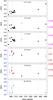 |
Fig. 1 Light curves in different energy ranges. On the x-axis, we report the last three digits of the Modified Julian Date. On the y-axis, on both left and right side, we report the count-rate. Black circles: XMM-Newton (0.3–0.5 keV, 0.5–2 keV, 2–10 keV); magenta nablas: Chandra (0.5–2 keV, 2–10 keV); red squares: NuSTAR (20–40 keV, 40–80 keV); blue triangles: INTEGRAL (20–40 keV, 40–80 keV, 80–300 keV). The vertical dotted lines highlight the seven observations we analysed in this paper (i.e., those including NuSTAR and/or INTEGRAL data). |
In Fig. 1, we show the light curves of all the fourteen XMM-Newton observations, the four NuSTAR observations and the five INTEGRAL observations of the campaign. The variability shown by the light curves in the low-energy ranges is mainly due to obscuration, as shown in Sect. 3. We will also show that the primary emission exhibits intrinsic variations as well, which explain the variability observed at higher energies. We refer the reader to Mehdipour et al. (2015) for the full time-line of the campaign (see their Fig. 1).
3. Spectral analysis
Spectral analysis and model fitting was carried out with the xspec 12.8 package (Arnaud 1996), using the χ2 minimisation technique throughout. In this paper, all errors are quoted at the 90% confidence level.
3.1. Spectral curvature above 10 keV
In Fig. 2 we plot for comparison the four NuSTAR/FPMA spectra above 10 keV, simultaneously fitted with a power law with tied parameters (χ2/d.o.f. = 1549/1178). The photon index obtained is Γ = 1.58 ± 0.02. The plot shows that the spectral variability in the hard X-rays during the campaign is not dramatic, while it is prominent in the soft X-rays (K14; Cappi et al., in prep.; di Gesu et al., in prep.) where obscuration plays a major role. After getting a general idea about the power law parameters, we tested the presence of spectral curvature by individually fitting each of the four NuSTAR spectra above 10 keV, first with a simple power law and as a second step including an exponential cut-off. The addition of the cut-off results in an improvement in all fits (Δχ2 ≲ −30), with a probability of chance improvement less than 10-8 according to the F-test. This result motivates the use of a cut-off power law in the analysis of the data. However, as a next step we test whether the spectral curvature is partly due to a reflection component.
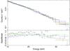 |
Fig. 2 Upper panel: 10–79 keV spectra of the four NuSTAR observations. Lower panel: residuals when simultaneously fitting with a power law. For clarity, we used only FPMA data, which are rebinned in the plot. |
3.2. The reflection component
To test for the presence of a reflection component, we fitted the data above 5 keV. By choosing 5 keV as a lower energy limit, we avoid the effects due to the strong absorption in the soft band. Good statistics are needed, so we only consider the four observations including NuSTAR data (obs. 2, 4, 5 and 6 of Table 1).
We fitted the XMM-Newton/pn, NuSTAR and INTEGRAL data simultaneously, leaving the cross-calibration constants free to vary. The normalization factors with respect to pn were always between 1 and 1.1. In particular, the spectral agreement between XMM-Newton and NuSTAR is generally good in their common 3–10 keV bandpass (Walton et al. 2013, 2014). We used a simple model, consisting of a cut-off power law modified by absorption, plus reflection. We included a neutral absorber with covering fraction fixed to 1, while the column density was free to vary. This is clearly an arbitrary choice, but the way we model the absorption, with a lower energy limit of 5 keV, does not affect the results that follow.
Following the analysis done by Cappi et al. (in prep.) and motivated by their detection of a neutral, narrow and constant Fe Kα line, we used the pexmon model (Nandra et al. 2007) in xspec for the reflection component. pexmon combines a neutral Compton reflection, as described by the pexrav model (Magdziarz & Zdziarski 1995) in xspec, with Fe Kα, Fe Kβ, Ni Kα lines and the Fe Kα Compton shoulder, generated self-consistently by Monte-Carlo simulations (George & Fabian 1991). We fixed the inclination angle of the reflector to 30 deg, appropriate for a type 1 source (e.g., Nandra et al. 1997) and consistent with past analyses of the Fe K lines in NGC 5548 (Yaqoob et al. 2001; Liu et al. 2010), but also with the inclination estimated for the broad-line region (Pancoast et al. 2014) and for the disk-corona system (Petrucci et al. 2000). The photon index, cut-off energy and normalization of the incident radiation were free to vary and not tied to those of the primary power law. This choice is justified a priori by the observed constancy of the Fe Kα line, and a posteriori by our constraints on the reflection component, which is consistent with being constant during the campaign. In this case, the distance of the reflecting material from the X-ray emitting region should be at least a few light months, i.e. a few ×104 gravitational radii, as we will discuss in Sect. 4.
The 90% contour plots of cut-off energy and normalization vs. photon index of pexmon are plotted in Figs. 3 and 4. The photon index and cut-off energy of the reflected continuum are not well constrained, however the contours are mutually consistent. The normalization vs. photon index contours are very similar for the four observations, with indication of a slightly larger normalization for obs. 6; nevertheless they are also marginally consistent with each other. These results are consistent with the reflected emission coming from remote material, and thus the parameters being constant during the campaign. For this reason, we chose to freeze hereafter the parameters of the reflection component to their weighted average derived from our analysis. We thus fixed the pexmon photon index to 1.9, cut-off energy to 300 keV and normalization to 5.5 × 10⁻³ (xspec units). The photon index of 1.9 is relatively high compared to the average value for NGC 5548, which is ~1.7 (see, e.g., Sobolewska & Papadakis 2009) but has indeed been observed in the past (Nandra et al. 1991; Reynolds 1997; Chiang et al. 2000). More importantly, the Swift monitoring discussed in Mehdipour et al. (in prep.) shows that the photon index reached 1.8–1.9 during most of 2012. Finally, from the pexmon parameters we estimate the average reflection fraction f as 0.3 ± 0.1, calculated as the ratio between the 20–40 keV flux illuminating the reflecting material and the 20–40 keV flux of the primary cut-off power law1. For a distant reflector, this ratio might not have a clear link with the covering factor as seen from the X-ray source (Malzac & Petrucci 2002), but this is discussed in more detail in Sect. 4.
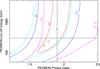 |
Fig. 3 pexmon cut-off energy vs. photon index 90% confidence level contours for the 4 NuSTAR observations, fitted above 5 keV. The grey solid lines indicate the values we chose to fix in the later broad-band analysis (1.9 for the photon index, 300 keV for the cut-off energy). |
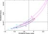 |
Fig. 4 pexmon normalization vs. photon index 90% confidence level contours for the 4 NuSTAR observations, fitted above 5 keV. The grey solid lines indicate the values we chose to fix in the later broad-band analysis (1.9 for the photon index, 5.5 × 10⁻³ for the normalization). |
3.3. Broad-band spectral analysis
Having obtained constraints on the parameters of the reflection component using the data above 5 keV, we now proceed to fit the total X-ray energy range available. We first use a phenomenological model, which is described below. Given the different satellites used in the seven observations, the energy range is limited to 0.5–79 keV for obs. 5 (Chandra/NuSTAR) and 0.3–79 keV for obs. 6 (XMM-Newton/NuSTAR). For all the other observations, the energy range is 0.3–400 keV, thanks to the addition of the INTEGRAL data.
3.3.1. The model components
Following Sects. 3.1 and 3.2, we modelled the continuum with a cut-off power law and the reflected component with pexmon, whose parameters were fixed. We describe in the following the other spectral components.
Obscuration:
the model presented by K14 includes two ionized, partially covering absorbers. Both were found to have a low degree of ionization, namely log ξ ≤ −4 and log ξ ≃ −1.2, such that at the EPIC-pn energy resolution they are almost equivalent to neutral absorbers. In particular, the absorber with log ξ = −1.2 was found to have a column density of 1.2 × 1022 cm-2 (K14) and such an absorber is indistinguishable, using pn data only, from a neutral one with a column density of 1.1 × 1022 cm-2. Since a detailed modelling of the obscuration is out of the scope of the present paper, we modelled the two absorbing components with pcfabs in xspec, which describes partial covering absorption by a neutral medium. Both the column density and the covering fraction of the two components were free to vary between different observations.
The warm absorber:
the model by K14 includes six warm absorber components, with different column densities (NH ~ 1020–1021 cm-2), ionization parameters (log ξ ~ 1–3), and outflow velocities (v ~ 250–1000 km s-1). We produced a table, with fixed parameters, from the best-fit model of the warm absorber derived by K14 and included it in xspec. For a comprehensive analysis of the UV properties of the warm absorber, see Arav et al. (2015).
The soft X-ray excess:
the physical origin of this component is still under debate, and it can be modelled with several different spectral models. The most common interpretations rely on relativistically blurred reflection (see, e.g., Crummy et al. 2006; Cerruti et al. 2011; Walton et al. 2012) or Comptonization by a warm medium (see, e.g., Petrucci et al. 2013; Boissay et al. 2014; Matt et al. 2014). Detailed modelling of the soft X-ray excess is beyond the scope of this paper, we thus followed the analysis done by Mehdipour et al. (in prep.) and assumed a thermal Comptonization component modelled by comptt (Titarchuk 1994) in xspec. The parameters of comptt were frozen, for each individual observation, to the values reported by Mehdipour et al. (in prep.), to which we refer the reader for details. We note that Mehdipour et al. (in prep.) found a significant flux variability of the soft excess between different observations, which we take into account here, but no apparent spectral shape variability.
Narrow emission lines:
a number of emission lines, such as [O VII] at 0.56 keV and [C V] at 0.3 keV, were detected in the XMM-Newton RGS spectra, as shown by K14. Again, we produced a table from the best-fit model and included it in xspec. These lines arguably originate from the Narrow-Line Region, therefore we do not expect line flux variations during the campaign (Peterson et al. 2013).
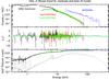 |
Fig. 5 Data and best-fit model for obs. 2 (XMM-Newton/NuSTAR/INTEGRAL, see Table 1). Upper panel: broad-band data and folded model. Middle panel: contribution to χ2. Lower panel: best-fit model E2f(E) with the plot of the various additive components, namely the cut-off power law, the reflection component, the soft excess and the narrow lines. |
3.3.2. Best-fit results
Best-fit parameters of the primary cut-off power law and the two absorbers (1) and (2), fitting the data down to 0.3 keV.
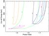 |
Fig. 6 Cut-off energy vs. primary photon index 90% confidence level contours for obs. 1 (black), obs. 2 (red), obs. 3 (green), obs. 4 (blue), obs. 5 (cyan), obs. 6 (magenta), obs. 7 (orange). |
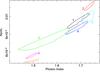 |
Fig. 7 Normalization vs. primary photon index 90% confidence level contours for obs. 1 (black), obs. 2 (red), obs. 3 (green), obs. 4 (blue), obs. 5 (cyan), obs. 6 (magenta), obs. 7 (orange). |
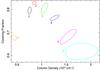 |
Fig. 8 Obscurer component 1: NH − CF 90% confidence level contours for obs. 1 (black), obs. 2 (red), obs. 3 (green), obs. 4 (blue), obs. 5 (cyan), obs. 6 (magenta), obs. 7 (orange). |
The best-fit parameters are reported in Table 2, while in Fig. 5 we show the data, residuals and best-fit model for obs. 2 (XMM-Newton/NuSTAR/INTEGRAL). The broad-band fit allows us to constrain the spectral shape more reliably with respect to the fit above 5 keV. In Figs. 6 and 7, we show the contour plots of the high-energy cut-off and normalization versus photon index, both for the primary continuum. The contours show significant variability of the photon index from ~1.5 (obs. 6, 7) to ~1.7 (obs. 1, 2, 4, 5). It should be noted that the photon index given in Kaastra et al. (2014), i.e. Γ = 1.566 ± 0.009, is a mean value which comes from the analysis of the co-added XMM-Newton and NuSTAR spectra of summer 2013. By including the individual NuSTAR and INTEGRAL high-energy spectra, we could constrain the photon index for each observation. Furthermore, the cut-off energy shows significant variability as well. We derive a lower limit for the cut-off energy in all the observations, and a measure of  keV for obs. 6. This measure is inconsistent, at 90% confidence level, with the lower limits determined from the other observations, with the exception of obs. 3. Finally, we note that the constraints we derived on the cut-off energy are mostly compatible with the average value estimated in Sect. 3.2 for the reflection component alone, i.e. 300 keV.
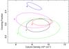 |
Fig. 9 Obscurer component 2: NH − CF 90% confidence level contours for obs. 1 (black), obs. 2 (red), obs. 3 (green), obs. 4 (blue), obs. 6 (magenta). This obscurer was not found in obs. 5 and 7. |
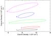 |
Fig. 10 NH − NH 90% confidence level contours for obs. 1 (black), obs. 2 (red), obs. 3 (green), obs. 4 (blue), obs. 6 (magenta). |
The broad-band fit helps constrain the obscurer components as well. In Figs. 8 and 9, we plot the contours of the covering fraction versus the column density of the two neutral absorbers, while in Fig. 10 we plot the contours of the two column densities versus each other. These contours show that absorption variability is statistically significant for both the low and high-NH absorbers. This can be seen, for example, by comparing obs. 2 (red contours) with obs. 4 (blue contours). Since the time interval between obs. 2 and 4 is ~10 days, we can conclude that the variability is significant on this time scale. In two cases, namely obs. 5 and 7, only one, low-NH absorber is needed, and adding the high-NH component does not improve the fit. For obs. 5 this can be explained by the lower sensitivity of Chandra HRC/LETG with respect to XMM-Newton EPIC-pn, which results in a lower signal-to-noise ratio in the soft band. For obs. 7, which is the last one and dated February 4, the absence of the high-NH component could simply mean that the source started changing back to the more usual, unobscured condition. However, for the model described above, we only obtain a relatively poor fit (χ2/ d.o.f. = 651 / 424), with strong, positive residuals around 0.5 keV, and negative residuals around 0.8 keV. We stress that the models we used for the warm absorber and the narrow emission lines were obtained from the analysis of pn and RGS data (K14), while our analysis is based on pn data alone. We may thus attribute such residuals in obs. 7 to a combination of the previously mentioned gain problem of the pn data with cross-calibration issues between the pn and RGS instruments (Kirsch et al. 2004). We obtained a much better fit (Δχ2 ≃ − 200) by adding a narrow Gaussian line with gauss in xspec, and an absorption edge with edge, without affecting the parameters of the primary cut-off power law. The emission line was found at E = 0.54 ± 0.01 keV, with an upper limit on the equivalent width of 20 eV. The absorption edge was found at E = 0.80 ± 0.01 keV with τ = 0.28 ± 0.06.
3.4. Test of Comptonization model
The last step of our analysis consists of fitting the average spectrum with a more realistic model, where the primary continuum is produced self-consistently via Comptonization of soft photons emitted by the disk. A more detailed analysis of the entire campaign with realistic Comptonization models is deferred to a future work.
First, we produced an average spectrum merging respectively the XMM-Newton, NuSTAR and INTEGRAL spectra used in this paper (Table 1) with the mathpha tool of heasoft. We then proceeded to fit this average spectrum over the range 0.3–400 keV, at first with the phenomenological model we have discussed above (Sect. 3.3.1). The resulting fit had χ2/d.o.f. = 3314/2631, with strong, positive residuals around 0.5 keV, and negative residuals around 0.6 keV (analogously to the already discussed obs. 7). We thus included two narrow Gaussian lines, with E = 0.53 ± 0.06 keV (in emission, equivalent width <50 eV) and E = 0.60 ± 0.02 keV (in absorption, equivalent width <20 eV). Again, we note that such residuals are most likely unphysical and due to cross-calibration between pn and RGS (Kirsch et al. 2004). However, the addition of these lines, while improving the fit, does not affect the best-fit parameters of the cut-off power law, namely Γ = 1.67 ± 0.02 and Ec> 250 keV, with χ2/d.o.f. = 3080/2627 and no prominent residual features. The relatively large χ2 is most likely an effect of averaging variable spectra (in particular in the soft band, due to absorption variability), and of the not perfect cross-calibration between XMM-Newton and NuSTAR, which especially appears in the co-added spectrum. We also note that XMM-Newton and NuSTAR do not cover strictly simultaneous times, since the exposure time of the two satellites is slightly different (see Table 1).
We then replaced the cut-off power law with the Comptonization model compps (Poutanen & Svensson 1996) in xspec. compps models the thermal Comptonization emission of a plasma cooled by soft photons with a disk black-body distribution. We chose a spherical geometry (parameter geom = −4 in compps) for the hot plasma and a temperature at the inner disk radius of 10 eV, fitting for the electron temperature kTe and Compton parameter y = 4τ(kTe/mec2). The best-fit parameters are reported in Table 3 and the kTe − y contour plot is shown in Fig. 11 (black contour). From the best-fit temperature kTe = 40 keV and parameter y = 0.85, we derive an optical depth  , where we estimate the errors from the kTe − y contour.
Best-fit parameters of the average data set, using the realistic Comptonization model compps for the continuum.
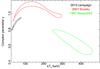 |
Fig. 11 kTe − y 90% confidence level contours for the spectra fitted with compps, using spherical geometry. Black: average spectrum of the 2013 campaign; red: average spectrum of the seven Suzaku observations taken in 2007; green: BeppoSAX observation taken in 1997. |
4. Discussion and conclusions
The broad-band coverage of the XMM-Newton, NuSTAR and INTEGRAL data allowed us to study the different components of the high-energy spectrum of NGC 5548 in detail.
First, we have been able to constrain the reflected component, which is consistent with being constant on a few months time scale, while the primary emission exhibits significant variability on a few days time scale. For example, the flux in the 2–10 keV band exhibits variations up to a factor of two over about 5 days during the campaign, with an outburst of several days duration in August-September (Mehdipour et al. 2015, see their Fig. 2). The lack of variability of the reflection component indicates that reflection is produced by cold and distant matter, lying at least a few light months away from the central X-ray source. This is consistent with the analysis of the Fe Kα line by Cappi et al. (in prep.) and with the absence of a significant contribution from relativistic reflection in this source (see, e.g., Brenneman et al. 2012). The lower limit of the reflector distance is consistent with this material being in the putative dusty torus, as the dust sublimation radius is estimated to be ~5 light months (Crenshaw et al. 2003). Furthermore, our results can be compared with past observations of the source. For this we focus on the 1997 BeppoSAX observation of NGC 5548 (Nicastro et al. 2000; Petrucci et al. 2000) and the average of seven Suzaku observations conducted in 2007 (Liu et al. 2010). In both cases, we re-fitted the archival data above 5 keV following the procedure described in Sect. 3.2. For the reflection component, we find that the spectral shape is always consistent with our best-fit parameters, i.e. a photon index of 1.9 and cut-off energy of 300 keV, while the reflected flux shows significant variations of about 50%. The primary flux (e.g., in the 2–10 keV band) shows similar variations, and we obtain a reflection fraction f consistent with that found during the 2013 campaign, i.e. f ~ 0.3, again calculated as the ratio between the illuminating and primary flux in the 20–40 keV range (see end of Sect. 3.2). Since f is consistent with being constant over a few years, the reflecting material should lie within a few light years from the primary X-ray source. In this case, the reflection fraction is indicative of the covering fraction of the reflector as seen from the X-ray source. From the definition of f, it follows that f = Ω / (4π − Ω). According to our results, then, the solid angle covered by the reflecting material can be estimated as Ω ≃ π, consistently with previous findings (e.g., Nandra & Pounds 1994; Pounds et al. 2003).
Then, we have been able to constrain the primary continuum and the effects of absorption. The primary continuum is well fitted by a power law with a photon index varying between ~1.5 and ~1.7, with at least a lower limit on the presence of a high-energy cut-off (Ec> 50 keV), which is usually considered a manifestation of Comptonization and is expected to be linked to the coronal temperature. The approximate relation between the temperature kTe of an optically thick Comptonizing corona and the cut-off energy Ec is kTe = Ec/ 3 (Petrucci et al. 2001). However, it should be noted that the cut-off of realistic Comptonization models is very different from an exponential cut-off. Moreover, the estimate of the temperature and of the optical depth also depends on the geometry assumed. In one case (obs. 6) we have obtained a measure of keV for the cut-off energy, which provides an estimate of  keV for the coronal temperature, with the caveats we just mentioned. Moreover, our results suggest a statistically significant variation of both the photon index and the cut-off energy. For example, in the case of obs. 5 we find a lower limit of 180 keV for the cut-off energy. We can thus estimate the coronal temperature to be >60 keV for obs. 5 and <37 keV for obs. 6, both at 90% confidence level. Such a variation may be due to different reasons, like a variation of the disk-corona geometry. The coronal optical depth and temperature should follow a univocal relationship for a given heating/cooling ratio, i.e. the ratio of the power dissipated in the corona to the intercepted soft luminosity which cools the electrons via Comptonization (Haardt & Maraschi 1991; Haardt et al. 1994, 1997). If the coronal optical depth changes, due for instance to a change in the accretion rate, the temperature will change accordingly, to keep the heating/cooling ratio constant. But the heating/cooling ratio can also change, responding to a variation in the disk-corona geometry, like a variation of the inner disk radius or a velocity variation of a potentially outflowing corona (Malzac et al. 2001). Then, the coronal optical depth and temperature will change in a non-trivial way to be consistent with the new heating/cooling ratio. Owing to these complexities, fitting the data with a phenomenological cut-off power law does not allow for a unique interpretation. However, our findings motivate us to apply realistic Comptonization models to constrain the coronal parameters.
Concerning absorption, we needed to add two different partially covering components (only one in two cases out of seven). The obscurer component 1 has NH ~ 1 × 1022 cm-2 and CF ~ 0.8, while the obscurer component 2 has NH ~ 9 × 1022 cm-2 and CF ~ 0.3, consistently with the estimates of K14. Both show significant variability on a time-scale of a few days, indicating that the obscuring material varies along the line of sight. This relatively heavy obscuration was unexpected, since NGC 5548 is historically thought to be an archetypal unobscured Seyfert 1. The discussion reported in K14 ascribes this obscuration to a fast and massive outflow which may be interpreted as a disk wind.
Finally, we have made a first step towards a more physical description of the primary emission by replacing the simple cut-off power law with a thermal Comptonization model to fit the average spectrum. According to our analysis, the X-ray emitting corona has a mean temperature of  keV and an optical depth of
  , assuming a spherical geometry, during this campaign. We compared this result with past observations of NGC 5548 by re-fitting the 1997 BeppoSAX spectrum and the 2007 Suzaku average spectrum. We used the compps model with spherical geometry (geom = −4) like we did in Sect. 3.4. The kTe − y contours are shown in Fig. 11. We find that the temperature and the optical depth are not consistent, at 90% confidence level, between the different observations. According to this test, the average values of the coronal temperature and optical depth show a significant long-term variability, namely over 10–15 years, with a clear decrease of the coronal temperature from about 300–400 keV in 1997 down to 40–50 keV in 2013. The optical depth, on the other hand, increases from about 0.2–0.3 up to 2–3. Although the values quoted are specific to the assumed spherical geometry for the corona, the changes in temperature and optical depth are significant if one were to assume a different geometry for the corona. The corresponding variation of the Compton parameter y suggests a variation, of uncertain origin, of the coronal heating/cooling ratio between these different observations. The coronal parameters may be variable on shorter time scales as well, as suggested by the detected variations of the cut-off energy.
Comparing with the 1997 BeppoSAX observation and the 2007 Suzaku observations, the 2013 campaign provided us a broader energy range which, together with the high signal-to-noise ratio spectra, allows for much better constraints on the coronal parameters (as shown by the contours in Fig. 11). However, for the optimal study of Comptonization, UV spectra may give a significant contribution. For example, Petrucci et al. (2013) have been able to fit the UV and soft X-ray spectra of Mrk 509 with a Comptonization component interpreted as a “warm” corona above the disk. If this scenario is also valid for NGC 5548, we expect a correlation between the UV and soft X-ray emission. This correlation can only be detected after the variability of the obscurer is properly removed. The analysis of the UV and soft X-ray emission by Mehdipour et al. (in prep.) indeed suggests that such a correlation is present, and that it may be intrinsically similar to that of Mrk 509. This point, and a thorough test of realistic Comptonization models, will be the subject of a forthcoming paper.
This definition is slightly different from the traditional R = Ω / 2π, where Ω is the solid angle subtended by the reflector (Magdziarz & Zdziarski 1995).
Acknowledgments
We are grateful to the anonymous referee for his/her helpful comments, which have improved the manuscript. This work is based on observations obtained with: the NuSTAR mission, a project led by the California Institute of Technology, managed by the Jet Propulsion Laboratory and funded by NASA; INTEGRAL, an ESA project with instrument and science data center funded by ESA member states (especially the PI countries: Denmark, France, Germany, Italy, Switzerland, Spain), Czech Republic, and Poland and with the participation of Russia and the USA; XMM-Newton, an ESA science mission with instruments and contributions directly funded by ESA Member States and the USA (NASA). The data used in this research are stored in the public archives of the international space observatories involved. This research has made use of data, software and/or web tools obtained from NASA’s High Energy Astrophysics Science Archive Research Center (HEASARC), a service of Goddard Space Flight Center and the Smithsonian Astrophysical Observatory. F.U., P.O.P., G.M., and S.B. acknowledge support from the French-Italian International Project of Scientific Collaboration: PICS-INAF project number 181542. F.U., P.O.P. acknowledge support from CNES. F.U. acknowledges support from Université Franco-Italienne (Vinci Ph.D. fellowship). F.U., G.M. acknowledges financial support from the Italian Space Agency under grant ASI/INAF I/037/12/0-011/13. G.A.K. was supported by NASA through grants for HST program number 13184 from the Space Telescope Science Institute, which is operated by the Association of Universities for Research in Astronomy, Incorporated, under NASA contract NAS5-26555. B.M.P. acknowledges support from the US NSF through grant AST-1008882. G.P. acknowledges support via an E.U. Marie Curie Intra-European fellowship under contract no. FP-PEOPLE-2012-IEF- 331095. K.C.S. acknowledges financial support from the Fondo Fortalecimiento de la Productividad Científica VRIDT 2013. We acknowledge support by ISSI in Bern; The Netherlands Organization for Scientific Research; the UK STFC; the French CNES, CNRS/PICS and CNRS/PNHE; the Swiss SNSF; the Italian INAF/PICS; the German Bundesministerium für Wirtschaft und Technologie/Deutsches Zentrum für Luft- und Raumfahrt (BMWI/DLR, FKZ 50 OR 1408); we acknowledge support from the Italian Space Agency under grants ASI-INAF I/037/12/P1 and ASI/INAF NuSTAR I/037/12/0.
References
- Arav, N., Chamberlain, C., Kriss, G. A., et al. 2015, A&A, 577, A37 (Paper II) [NASA ADS] [CrossRef] [EDP Sciences] [Google Scholar]
- Arnaud, K. A. 1996, in Astronomical Data Analysis Software and Systems V, eds. G. H. Jacoby, & J. Barnes, ASP Conf Ser., 101, 17 [Google Scholar]
- Ballantyne, D. R., Bollenbacher, J. M., Brenneman, L. W., et al. 2014, ApJ, 794, 62 [NASA ADS] [CrossRef] [Google Scholar]
- Bianchi, S., Guainazzi, M., Matt, G., Fonseca Bonilla, N., & Ponti, G. 2009, A&A, 495, 421 [NASA ADS] [CrossRef] [EDP Sciences] [Google Scholar]
- Boissay, R., Paltani, S., Ponti, G., et al. 2014, A&A, 567, A44 [NASA ADS] [CrossRef] [EDP Sciences] [Google Scholar]
- Brenneman, L. W., Elvis, M., Krongold, Y., Liu, Y., & Mathur, S. 2012, ApJ, 744, 13 [NASA ADS] [CrossRef] [Google Scholar]
- Brenneman, L. W., Madejski, G., Fuerst, F., et al. 2014, ApJ, 788, 61 [NASA ADS] [CrossRef] [Google Scholar]
- Cerruti, M., Ponti, G., Boisson, C., et al. 2011, A&A, 535, A113 [NASA ADS] [CrossRef] [EDP Sciences] [Google Scholar]
- Chiang, J., Reynolds, C. S., Blaes, O. M., et al. 2000, ApJ, 528, 292 [NASA ADS] [CrossRef] [Google Scholar]
- Courvoisier, T. J.-L., Walter, R., Beckmann, V., et al. 2003, A&A, 411, L53 [NASA ADS] [CrossRef] [EDP Sciences] [Google Scholar]
- Crenshaw, D. M., Kraemer, S. B., Gabel, J. R., et al. 2003, ApJ, 594, 116 [NASA ADS] [CrossRef] [Google Scholar]
- Crummy, J., Fabian, A. C., Gallo, L., & Ross, R. R. 2006, MNRAS, 365, 1067 [NASA ADS] [CrossRef] [Google Scholar]
- de Vaucouleurs, G., de Vaucouleurs, A., Corwin, Jr., H. G., et al. 1991, Third Reference Catalogue of Bright Galaxies, Vol. I: Explanations and references, Vol. II: Data for galaxies between 0h and 12h, Vol. III: Data for galaxies between 12h and 24h [Google Scholar]
- Done, C., Davis, S. W., Jin, C., Blaes, O., & Ward, M. 2012, MNRAS, 420, 1848 [NASA ADS] [CrossRef] [Google Scholar]
- George, I. M., & Fabian, A. C. 1991, MNRAS, 249, 352 [NASA ADS] [CrossRef] [Google Scholar]
- Haardt, F., & Maraschi, L. 1991, ApJ, 380, L51 [NASA ADS] [CrossRef] [Google Scholar]
- Haardt, F., Maraschi, L., & Ghisellini, G. 1994, ApJ, 432, L95 [NASA ADS] [CrossRef] [Google Scholar]
- Haardt, F., Maraschi, L., & Ghisellini, G. 1997, ApJ, 476, 620 [NASA ADS] [CrossRef] [Google Scholar]
- Harrison, F. A., Craig, W. W., Christensen, F. E., et al. 2013, ApJ, 770, 103 [NASA ADS] [CrossRef] [Google Scholar]
- Kaastra, J. S., Petrucci, P.-O., Cappi, M., et al. 2011, A&A, 534, A36 [NASA ADS] [CrossRef] [EDP Sciences] [Google Scholar]
- Kaastra, J. S., Kriss, G. A., Cappi, M., et al. 2014, Science, 345, 64 [NASA ADS] [CrossRef] [Google Scholar]
- Kirsch, M. G. F., Altieri, B., Chen, B., et al. 2004, in UV and Gamma-Ray Space Telescope Systems, eds. G. Hasinger, & M. J. L. Turner, SPIE Conf. Ser., 5488, 103 [Google Scholar]
- Liu, Y., Elvis, M., McHardy, I. M., et al. 2010, ApJ, 710, 1228 [NASA ADS] [CrossRef] [Google Scholar]
- Magdziarz, P. & Zdziarski, A. A. 1995, MNRAS, 273, 837 [NASA ADS] [CrossRef] [Google Scholar]
- Malizia, A., Molina, M., Bassani, L., et al. 2014, ApJ, 782, L25 [NASA ADS] [CrossRef] [Google Scholar]
- Malzac, J., & Petrucci, P.-O. 2002, MNRAS, 336, 1209 [NASA ADS] [CrossRef] [Google Scholar]
- Malzac, J., Beloborodov, A. M., & Poutanen, J. 2001, MNRAS, 326, 417 [NASA ADS] [CrossRef] [Google Scholar]
- Marinucci, A., Matt, G., Kara, E., et al. 2014, MNRAS, 440, 2347 [NASA ADS] [CrossRef] [Google Scholar]
- Matt, G., Marinucci, A., Guainazzi, M., et al. 2014, MNRAS, 439, 3016 [NASA ADS] [CrossRef] [Google Scholar]
- Mehdipour, M., Branduardi-Raymont, G., Kaastra, J. S., et al. 2011, A&A, 534, A39 [NASA ADS] [CrossRef] [EDP Sciences] [Google Scholar]
- Mehdipour, M., Kaastra, J. S., Kriss, G. A., et al. 2015, A&A, 575, A22 (Paper I) [NASA ADS] [CrossRef] [EDP Sciences] [Google Scholar]
- Nandra, K. & Pounds, K. A. 1994, MNRAS, 268, 405 [NASA ADS] [CrossRef] [Google Scholar]
- Nandra, K., Pounds, K. A., Stewart, G. C., et al. 1991, MNRAS, 248, 760 [NASA ADS] [CrossRef] [Google Scholar]
- Nandra, K., George, I. M., Mushotzky, R. F., Turner, T. J., & Yaqoob, T. 1997, ApJ, 477, 602 [NASA ADS] [CrossRef] [Google Scholar]
- Nandra, K., O’Neill, P. M., George, I. M., & Reeves, J. N. 2007, MNRAS, 382, 194 [NASA ADS] [CrossRef] [Google Scholar]
- Nicastro, F., Piro, L., De Rosa, A., et al. 2000, ApJ, 536, 718 [NASA ADS] [CrossRef] [Google Scholar]
- Pancoast, A., Brewer, B. J., Treu, T., et al. 2014, MNRAS, 445, 3073 [NASA ADS] [CrossRef] [Google Scholar]
- Perola, G. C., Matt, G., Cappi, M., et al. 2002, A&A, 389, 802 [Google Scholar]
- Peterson, B. M., Denney, K. D., De Rosa, G., et al. 2013, ApJ, 779, 109 [NASA ADS] [CrossRef] [Google Scholar]
- Petrucci, P. O., Haardt, F., Maraschi, L., et al. 2000, ApJ, 540, 131 [NASA ADS] [CrossRef] [Google Scholar]
- Petrucci, P. O., Haardt, F., Maraschi, L., et al. 2001, ApJ, 556, 716 [NASA ADS] [CrossRef] [Google Scholar]
- Petrucci, P.-O., Paltani, S., Malzac, J., et al. 2013, A&A, 549, A73 [NASA ADS] [CrossRef] [EDP Sciences] [Google Scholar]
- Ponti, G., Papadakis, I., Bianchi, S., et al. 2012, A&A, 542, A83 [NASA ADS] [CrossRef] [EDP Sciences] [Google Scholar]
- Pounds, K. A., Reeves, J. N., Page, K. L., et al. 2003, MNRAS, 341, 953 [NASA ADS] [CrossRef] [Google Scholar]
- Poutanen, J., & Svensson, R. 1996, ApJ, 470, 249 [NASA ADS] [CrossRef] [Google Scholar]
- Reis, R. C., & Miller, J. M. 2013, ApJ, 769, L7 [Google Scholar]
- Reynolds, C. S. 1997, MNRAS, 286, 513 [NASA ADS] [CrossRef] [Google Scholar]
- Sobolewska, M. A. & Papadakis, I. E. 2009, MNRAS, 399, 1597 [NASA ADS] [CrossRef] [Google Scholar]
- Steenbrugge, K. C., Kaastra, J. S., Crenshaw, D. M., et al. 2005, A&A, 434, 569 [NASA ADS] [CrossRef] [EDP Sciences] [Google Scholar]
- Titarchuk, L. 1994, ApJ, 434, 570 [NASA ADS] [CrossRef] [Google Scholar]
- Walton, D. J., Nardini, E., Fabian, A. C., Gallo, L. C., & Reis, R. C. 2012, MNRAS, 428, 2901 [Google Scholar]
- Walton, D. J., Fuerst, F., Harrison, F., et al. 2013, ApJ, 779, 148 [NASA ADS] [CrossRef] [Google Scholar]
- Walton, D. J., Harrison, F. A., Grefenstette, B. W., et al. 2014, ApJ, 793, 21 [NASA ADS] [CrossRef] [Google Scholar]
- Winkler, C., Courvoisier, T. J.-L., Di Cocco, G., et al. 2003, A&A, 411, L1 [NASA ADS] [CrossRef] [EDP Sciences] [Google Scholar]
- Yaqoob, T., George, I. M., Nandra, K., et al. 2001, ApJ, 546, 759 [NASA ADS] [CrossRef] [Google Scholar]
All Tables
Logs of the simultaneous XMM-Newton, NuSTAR, and/or INTEGRAL observations of NGC 5548 during our campaign.
Best-fit parameters of the primary cut-off power law and the two absorbers (1) and (2), fitting the data down to 0.3 keV.
Best-fit parameters of the average data set, using the realistic Comptonization model compps for the continuum.
All Figures
|
Fig. 1 Light curves in different energy ranges. On the x-axis, we report the last three digits of the Modified Julian Date. On the y-axis, on both left and right side, we report the count-rate. Black circles: XMM-Newton (0.3–0.5 keV, 0.5–2 keV, 2–10 keV); magenta nablas: Chandra (0.5–2 keV, 2–10 keV); red squares: NuSTAR (20–40 keV, 40–80 keV); blue triangles: INTEGRAL (20–40 keV, 40–80 keV, 80–300 keV). The vertical dotted lines highlight the seven observations we analysed in this paper (i.e., those including NuSTAR and/or INTEGRAL data). |
| In the text | |
|
Fig. 2 Upper panel: 10–79 keV spectra of the four NuSTAR observations. Lower panel: residuals when simultaneously fitting with a power law. For clarity, we used only FPMA data, which are rebinned in the plot. |
| In the text | |
|
Fig. 3 pexmon cut-off energy vs. photon index 90% confidence level contours for the 4 NuSTAR observations, fitted above 5 keV. The grey solid lines indicate the values we chose to fix in the later broad-band analysis (1.9 for the photon index, 300 keV for the cut-off energy). |
| In the text | |
|
Fig. 4 pexmon normalization vs. photon index 90% confidence level contours for the 4 NuSTAR observations, fitted above 5 keV. The grey solid lines indicate the values we chose to fix in the later broad-band analysis (1.9 for the photon index, 5.5 × 10⁻³ for the normalization). |
| In the text | |
|
Fig. 5 Data and best-fit model for obs. 2 (XMM-Newton/NuSTAR/INTEGRAL, see Table 1). Upper panel: broad-band data and folded model. Middle panel: contribution to χ2. Lower panel: best-fit model E2f(E) with the plot of the various additive components, namely the cut-off power law, the reflection component, the soft excess and the narrow lines. |
| In the text | |
|
Fig. 6 Cut-off energy vs. primary photon index 90% confidence level contours for obs. 1 (black), obs. 2 (red), obs. 3 (green), obs. 4 (blue), obs. 5 (cyan), obs. 6 (magenta), obs. 7 (orange). |
| In the text | |
|
Fig. 7 Normalization vs. primary photon index 90% confidence level contours for obs. 1 (black), obs. 2 (red), obs. 3 (green), obs. 4 (blue), obs. 5 (cyan), obs. 6 (magenta), obs. 7 (orange). |
| In the text | |
|
Fig. 8 Obscurer component 1: NH − CF 90% confidence level contours for obs. 1 (black), obs. 2 (red), obs. 3 (green), obs. 4 (blue), obs. 5 (cyan), obs. 6 (magenta), obs. 7 (orange). |
| In the text | |
|
Fig. 9 Obscurer component 2: NH − CF 90% confidence level contours for obs. 1 (black), obs. 2 (red), obs. 3 (green), obs. 4 (blue), obs. 6 (magenta). This obscurer was not found in obs. 5 and 7. |
| In the text | |
|
Fig. 10 NH − NH 90% confidence level contours for obs. 1 (black), obs. 2 (red), obs. 3 (green), obs. 4 (blue), obs. 6 (magenta). |
| In the text | |
|
Fig. 11 kTe − y 90% confidence level contours for the spectra fitted with compps, using spherical geometry. Black: average spectrum of the 2013 campaign; red: average spectrum of the seven Suzaku observations taken in 2007; green: BeppoSAX observation taken in 1997. |
| In the text | |
Current usage metrics show cumulative count of Article Views (full-text article views including HTML views, PDF and ePub downloads, according to the available data) and Abstracts Views on Vision4Press platform.
Data correspond to usage on the plateform after 2015. The current usage metrics is available 48-96 hours after online publication and is updated daily on week days.
Initial download of the metrics may take a while.