| Issue |
A&A
Volume 577, May 2015
|
|
|---|---|---|
| Article Number | A116 | |
| Number of page(s) | 14 | |
| Section | Extragalactic astronomy | |
| DOI | https://doi.org/10.1051/0004-6361/201425381 | |
| Published online | 13 May 2015 | |
SN 2013dx associated with GRB 130702A: a detailed photometric and spectroscopic monitoring and a study of the environment⋆,⋆⋆
1 INAF–Osservatorio Astronomico di Roma, via Frascati 33, 00040 Monteporzio Catone, Italy
e-mail: This email address is being protected from spambots. You need JavaScript enabled to view it.
2 ASI-Science Data Center, via del Politecnico snc, 00133 Rome, Italy
3 INAF–Istituto di Astrofisica Spaziale e Fisica Cosmica, via P. Gobetti 101, 40129 Bologna, Italy
4 Scuola Normale Superiore, Piazza dei Cavalieri 7, 56126 Pisa, Italy
5 INAF–Osservatorio Astronomico di Brera, via E. Bianchi 46, 23807 Merate (LC), Italy
6 INAF–Osservatorio Astronomico di Capodimonte, Salita Moiariello 16, 80131 Napoli, Italy
7 ICRANET, Piazza della Republica 10, 65122 Pescara, Italy
8 ARI, Liverpool John Moores University, IC2 Liverpool Science Park 146 Brownlow Hill, Liverpool, L3 5RF, UK
9 INAF–Osservatorio Astronomico di Padova, Vicolo dell’Osservatorio 5, 35122 Padova, Italy
10 Max-Planck Institute for Astrophysics, Garching, Karl-Schwarzschild-Str. 1, Postfach 1317, 85741 Garching, Germany
11 Millennium Institute of Astrophysics, Casilla 36-D, Santiago, Chile
12 Departamento de Ciencias Fisicas, Universidad Andres Bello, Avda. Republica 252, Santiago, Chile
13 Dark Cosmology Center, Niels Bohr Institute, University of Copenhagen, Juliane Maries Vej 30, 2100 Copenhagen, Denmark
14 European Southern Observatory, Karl-Schwarzschild-Strasse 2, 85748 Garching bei München, Germany
Received: 20 November 2014
Accepted: 17 February 2015
Abstract
Aims. Long-duration gamma-ray bursts (GRBs) and broad-line, type Ic supernovae (SNe) are strongly connected. We aim at characterizing SN 2013dx, which is associated with GRB 130702A, through a sensitive and extensive ground-based observational campaign in the optical-IR band.
Methods. We monitored the field of the Swift GRB 130702A (redshift z = 0.145) using the 8.2 m VLT, the 3.6 m TNG and the 0.6 m REM telescopes during the time interval between 4 and 40 days after the burst. Photometric and spectroscopic observations revealed the associated type Ic SN 2013dx. Our multiband photometry allowed constructing a bolometric light curve.
Results. The bolometric light curve of SN 2013dx resembles that of 2003dh (associated with GRB 030329), but is ~10% faster and ~25% dimmer. From this we infer a synthesized 56Ni mass of ~0.2 M⊙. The multi-epoch optical spectroscopy shows that the SN 2013dx behavior is best matched by SN 1998bw, among the other well-known low-redshift SNe associated with GRBs and XRFs, and by SN 2010ah, an energetic type Ic SN not associated with any GRB. The photospheric velocity of the ejected material declines from ~2.7 × 10⁴ km s-1 at 8 rest frame days from the explosion, to ~3.5 × 10³ km s-1 at 40 days. These values are extremely close to those of SN1998bw and 2010ah. We deduce for SN 2013dx a kinetic energy of ~35 × 1051 erg and an ejected mass of ~7 M⊙. This suggests that the progenitor of SN2013dx had a mass of ~25–30 M⊙, which is 15–20% less massive than that of SN 1998bw. Finally, we studied the SN 2013dx environment through spectroscopy of the closeby galaxies: 9 out of the 14 inspected galaxies lie within 0.03 in redshift from z = 0.145, indicating that the host of GRB 130702A/SN 2013dx belongs to a group of galaxies, an unprecedented finding for a GRB-associated SN and, to our knowledge, for long GRBs in general.
Key words: gamma-ray burst: general / supernovae: individual: SN 2013dx
Based on observations collected at the Italian 3.6-m Telescopio Nazionale Galileo (TNG), operated on the island of La Palma by the Fundacion Galileo Galilei of the INAF (Instituto Nazionale di Astrofisica) at the Spanish Observatorio del Roque de los Muchachos of the Instituto de Astrofisica de Canarias under program A27TAC 5, and at the European Southern Observatory, ESO, the VLT/Antu telescope, Paranal, Chile, proposal code: 291.D-5032(A).
Appendix A is available in electronic form at http://www.aanda.org
© ESO, 2015
1. Introduction
The connection between gamma-ray bursts (GRBs) and supernovae (SNe) has been firmly established on the basis of a handful of nearby events (z< 0.3) for which a decent spectroscopic monitoring was possible (Galama et al. 1998; Patat et al. 2001; Hjorth et al. 2003; Stanek et al. 2003; Malesani et al. 2004; Pian et al. 2006; Modjaz et al. 2006; Bufano et al. 2012), which enabled deriving the physical properties of the SNe (Mazzali et al. 2006a,b; Woosley & Bloom 2006; Hjorth & Bloom 2012).
In these few cases, observations have revealed that SNe accompanying GRBs are explosions of bare stellar cores, that is, their progenitors (whose estimated mass is higher than ~20 M⊙) have lost all their hydrogen and helium envelopes before collapse (a.k.a. supernovae of type Ic). A stripped star of Wolf-Rayet type (Crowther 2007) appears indeed more suited to favor the propagation of a relativistic jet. However, many unknowns still surround the GRB-SN connection: the properties of their progenitors (e.g., their multiplicity and metallicity, Podsiadlowski et al. 2010; Levesque et al. 2014), the nature of their remnants (e.g., Woosley & Heger 2012; Mazzali et al. 2014), and the formation and propagation of the jets through the stellar envelope (Zhang et al. 2003; Uzdensky & MacFadyen 2006; Fryer et al. 2009; Lyutikov 2011; Bromberg et al. 2014).
The detailed analysis of the physics of the supernovae can elucidate these problems, and accurate optical spectroscopy is a fundamental tool to this aim. It is well known, in fact, that light curve models alone do not have the ability to uniquely determine all supernova parameters. In particular, while the mass of 56Ni can be reasonably well established from the light-curve peak if the time of explosion is known to within a good accuracy, or from the late, exponential decline phase of the light curve if this is observed, the two parameters that determine the shape of the light curve, the ejecta mass Mej and the kinetic energy EK, are degenerate (Eq. (2); Arnett 1982). Only the simultaneous use of light curve and spectra can break this degeneracy (Mazzali et al. 2013, and references therein).
Time-resolved optical spectra of GRB-SNe can be acquired only at z ≲ 0.3, however. At higher redshift, the subtraction of the host galaxy and afterglow components from the spectrum of the GRB optical counterpart lowers the signal-to-noise ratio (S/N) dramatically, so that the resulting spectral residuals are noisy (e.g., Melandri et al. 2012, 2014). In fact, in the redshift range 0.3 ≲ z ≲ 1 the current generation of telescopes can test the SN-GRB connection only on the basis of a single spectrum acquired at the epoch of maximum light (Della Valle et al. 2003; Soderberg et al. 2005; Berger et al. 2011; Sparre et al. 2011; Jin et al. 2013; Cano et al. 2014) or through the detection of rebrightenings in the GRB afterglow light-curves, due to emerging SNe (e.g. Bloom et al. 1999; Lazzati et al. 2001; Greiner et al. 2003; Garnavich et al. 2003; Masetti et al. 2003; Zeh et al. 2004; Gorosabel et al. 2005; Bersier et al. 2006; Della Valle et al. 2006a,b; Soderberg et al. 2006, 2007; Cobb et al. 2010; Tanvir et al. 2010; Cano et al. 2011a,b, 2014). Finally, at redshift higher than one, even the detection of a rebrightening is in general not possible.
SN 2013dx, associated with GRB 130702A at z = 0.145, represents a remarkable new entry into the group of the most consistently investigated SN-GRB events. Here, we present the results of our extensive photometric and spectroscopic campaign, carried out with the VLT, TNG, and REM telescopes, covering an interval of about 40 days after GRB detection. In particular, we obtained 16 spectra spaced apart by 2–3 days.
The paper is organized as follows: Sect. 2 summarizes the properties of GRB 130702A and its associated SN 2013dx as reported in the literature; Sect. 3 introduces our dataset and illustrates the data reduction process; Sect. 4 presents our results; in Sect. 5 we draw our conclusions. We assume a cosmology with H0 = 70 km s-1 Mpc-1, Ωm = 0.3, ΩΛ = 0.7.
2. GRB 130702A/SN 2013 dx
GRB 130702A was detected by Fermi-LAT and -GBM instruments on July 02, 2013 at 00:05 UT (Fermi trigger 394416326, Cheung et al. 2013; Collazzi et al. 2013). In the following, this time represents our t0.
The intermediate Palomar Transient Factory reported a possible counterpart after following up the burst in the optical band at the position RA (J2000) = 14h29m14.78s Dec (J2000) = +15d46′26.4′′. The transient was 0.6′′ away from an SDSS faint source (r = 23.01) classified as a star, which was later identified as its host galaxy (Singer et al. 2013; Kelly et al. 2013). A Swift target-of-opportunity observation was then activated, and analysis of the XRT and UVOT data revealed a coincident, new X-ray source in the sky (D’Avanzo et al. 2013a). The fading behavior was confirmed both in the X-ray by subsequent XRT observations (D’Avanzo et al. 2013b) and in the optical bands by several ground-based telescopes (see, e.g., Guidorzi et al. 2013; Xu et al. 2013a, b; D’Avanzo et al. 2013b).
GRB 130702A was also observed by Konus-Wind in the 20–1200 keV band (Golenetskii et al. 2013) and by INTEGRAL (Hurley et al. 2013) in the mm (Perley & Kasliwal 2014) and in the radio band (van der Horst 2013).
The redshift of the transient was reported to be z = 0.145 (Mulchaey et al. 2013a; D’Avanzo et al. 2013c; Mulchaey et al. 2013b). The emerging of a new supernova associated with GRB 130702A was detected by several spectroscopic measurements (Schulze et al. 2013a; Cenko et al. 2013; D’Elia et al. 2013a), and was named SN 2013dx (Schulze et al. 2013b; D’Elia et al. 2013b).
3. Observations and data reduction
We observed the field of SN 2013dx in imaging and spectroscopic modes using VLT, TNG, and REM. Details on the data acquisition and reduction process are given below. Figure 1 shows the SN 2013dx field, with two nearby galaxies clearly visible. Details on the analysis of this field can be found in Sect. 4.6.
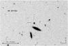 |
Fig. 1 SN 2013dx field acquired with VLT/FORS2 on July 27 in the R band. The SN and host galaxy position is indicated by two perpendicular markers. Two companion galaxies are clearly visible southward. |
3.1. Photometry
3.1.1. TNG photometry
TNG photometry was conducted using the DOLORES camera in imaging mode, with the SDSS g,r,i,z and the Johnson U filters. Image reduction was carried out by following the standard procedures: subtraction of an averaged bias frame, division by a normalized flat frame. Astrometry was performed using the USNOB1.01 catalogs. Aperture photometry was made with the Starlink2 PHOTOM package. The aperture was set to 10 pixels, which is equivalent to 2.5′′. The calibration was made against the SDSS catalog and Landolt standard field stars (for the U filter). To minimize any systematic effect, we performed differential photometry with respect to local isolated and non-saturated standard stars selected from these two catalogs.
The log of the TNG photometric observations can be found in Table 1.
Log of the TNG photometric observations.
3.1.2. VLT photometry
VLT photometry was carried out using the FORS2 camera in imaging mode with the Johnson U,B,R,I filters. Image reduction was performed using the same standard techniques as were adopted for the TNG data. Images were calibrated against Landolt standard field stars. Again, differential photometry was performed to minimize any systematic effects. The aperture was set to 10 pixels, which is equivalent to 1.3′′.
The log of the VLT photometric observations can be found in Table 2.
Log of the VLT photometric observations.
3.1.3. REM photometry
Optical and NIR observations were performed with the REM telescope (Zerbi et al. 2001; Chincarini et al. 2003; Covino et al. 2004) equipped with the ROSS2 optical imager and the REMIR NIR camera. The ROSS2 instrument is able to observe simultaneously in the g,r,i, and z SDSS filters. Observations of GRB 130702A/SN 2013dx were carried out over fifteen epochs between 2013 July 10 and Aug. 13. Image reduction was carried out by following the same standard procedures as for the TNG and VLT photometry, including differential photometry. The aperture was set to 10 pixels, which is equivalent to 5′′. Astrometry was performed using the USNOB1.0 and the 2MASS3 catalogs for the optical and NIR frames, respectively. The calibration was made against the SDSS catalog for the optical filters and the 2MASS catalog for NIR filters.
The log of the REM photometric observations can be found in Table 3, where we only report the g and r photometry. In the i band the S/N was too low, and the SN 2013dx too much contaminated by the host galaxy to obtain firm detections. In the z and H bands we did not detect the SN down to typical upper limits of z ~ 19.7 (AB, 3σ) and H ~ 18 (Vega, 3σ). The columns are organized in the same way as in Table 1.
Log of the REM photometric observations.
3.2. Spectroscopy
3.2.1. TNG spectroscopy
TNG spectroscopy was carried out using the DOLORES camera in slit mode, with the LR-B grism. This configuration covers the spectral range 3000–8430 Å with a resolution of λ/ Δλ = 585 for a slit width of 1′′ at the central wavelength 5850 Å. Spectra were acquired at five epochs. A slit width of 1′′ was used in all but the first observation, for which a 1.5′′ slit was adopted, owing to a seeing higher than 1′′. The slit position angle was set to the parallactic angle in all our observations. Table 4 contains a summary of the TNG spectroscopic observations.
The spectra were extracted using standard procedures (bias and background subtraction, flat fielding, wavelength and flux calibration) under the packages ESO-MIDAS4 and IRAF5. Ne-Hg or helium lamps and spectrophotometric stellar spectra acquired in the same nights as the target were used for wavelength and flux calibration.
To account for slit losses, we matched the flux-calibrated spectra with our multiband TNG photometry acquired in the same nights.
Log of the TNG spectroscopic observations.
3.2.2. VLT spectroscopy
VLT spectroscopy was carried out using the FORS2 camera in slit mode, with the 300V grism. This configuration covers the spectral range 3300–9500 Å with a resolution of λ/ Δλ = 440 for a slit width of 1′′ at the central wavelength 5900 Å. Eleven spectroscopic epochs were acquired. A slit width of 1′′ was used in all observations. The slit position angle was set to different values in each observation to place different field galaxies in the slit to study the SN 2013dx surroundings (see Sect. 4.6 for details). Table 5 gives a summary of the VLT spectroscopic observations.
As for the TNG data, the spectra were extracted using the packages ESO-MIDAS and IRAF. A He+Ag/Cd+Ar lamp and spectrophotometric stars acquired the same night of the target were used for wavelength and flux calibration. For a few epochs, some spectrophotometric stars were not observed in the same night as the target. In these cases, the flux calibration was performed using archival data. In none of these epochs, however, was the difference beween the observation time of the scientific files and the adopted standard longer than three days.
To account for slit losses, we checked the flux-calibrated spectra against our simultaneous VLT multiband photometry.
Log of the VLT spectroscopic observations.
4. Results
4.1. Optical light curves
Our optical photometric data, only corrected for Galactic extinction, are shown in Fig. 2. The SN component starts to emerge and dominate its host galaxy and GRB optical afterglow at about five days after the GRB explosion. We fit empirical curves to the data past day five to determine the peak times of SN2013dx in the different bands. The results in the rest frame are Tpeak,i = 16 ± 2 days, Tpeak,r = 15 ± 1 days, Tpeak,g = 10 ± 2 days, and Tpeak,U = 8 ± 1 days.
SN 2013dx is one of the few cases in which a SN is observed in the U band. The U peak is observed very early, at about one week in the rest-frame. As commonly observed in other SNe, the peak occurs at later times while moving to redder bands. As an example, the I-band peak is observed about a week later than that in the U-band.
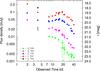 |
Fig. 2 GRB 130702A/SN2013dx optical and near-infrared light curves. The time origin t = 0 coincides with the GRB explosion time. |
4.2. Optical spectra
First, all the VLT and TNG optical spectra of SN 2013dx were dereddened using the Galactic value E(B − V) = 0.04 mag toward its line of sight (Schlegel et al. 1998). The intrinsic extinction appears to be negligible both from X-ray data and from analysis of the X-ray-to-optical spectral energy distribution. Then, we estimated the host galaxy contribution. Since SN 2013dx was still bright at the time of our last observation (10 Aug.) and later on its field became not observable anymore because of solar constraints, we could not acquire a reliable spectrum to subtract the host galaxy contribution from our data. Therefore, we considered the SDSS magnitudes of the host galaxy, u = 24.42 ± 0.96, g = 23.81 ± 0.85, r = 23.01 ± 0.24, i = 23.22 ± 0.39, and z = 23.04 ± 0.59, and noted that after they were reduced to rest-frame, they were consistent with the normalized template of a star-forming galaxy with moderate intrinsic absorption (E(B − V) < 0.10, Kinney et al. 1996). Then we subtracted this rescaled template from our dereddened fluxes. The host galaxy contributes about 15% of the total flux, and possibly less, because not all its light is captured in the slit when acquiring the SN spectra.
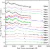 |
Fig. 3 Sixteen dereddened, host- and afterglow-subtracted TNG and VLT spectra. For clarity, the spectra have been vertically shifted by 2 × 10-17 erg cm-2 s-1 Å-1, with the earliest one (TNG, Jul. 9) at top and the latest one, not shifted, at the bottom. All VLT spectra are smoothed with a boxcar of 8 Å, with the exception of those from Jul. 20 and 22 (that have the lowest S/N), which are smoothed by 25 Å. All TNG spectra are smoothed with a boxcar of 7 Å. The time intervals are computed from the GRB explosion time. Black filled circles mark the position of the SiII6355 feature, used to determine the photospheric velocity of the ejecta (see Sect. 4.4). |
Finally, we subtracted the afterglow contribution. The afterglow light curve can be modeled with a broken power law, as shown in Singer et al. (2013). We thus adopted their first decay index (α1 = 0.57) and their temporal break tb = 1.17 days. However, the second decay index α2 does not take into account the emerging SN contribution. α2 = 1.85 is the lowest index for which the afterglow is not oversubtracted in our early time photometry, while α2 = 2.5 is the highest index allowed by the closure relations linking spectral and temporal indices (Zhang & Mészáros 2004). Thus, we chose an average α2 = 2.2. The adopted spectral index is βν = 0.7 (Singer et al. 2013). Even assuming the two extreme decay indices, the difference in the afterglow contribution can only be appreciated in the first three spectra, and it is lower than 20% in the worst case.
Figure 3 shows our sixteen dereddened, host- and afterglow-subtracted TNG and VLT spectra. The spectra are shown starting from 4000 Å in the rest-frame, because the flux calibration becomes unreliable at shorter wavelengths.
In Fig. 4 we compare in the rest-frame 11 of our spectra with those of SN 1998bw at comparable phases after explosion (Patat et al. 2001). Each SN 1998bw spectrum is scaled in flux by an arbitrary constant to find the best match with our spectral dataset. In most pairs of spectra the same continuum shape and broad absorption features can be seen, even if some diversities are present (at t< 20 d the 4400 Å pseudo-emission peak is completely absent in 1998bw; the pseudo-peak around 6300 Å in 1998bw is absent in 2013dx; the strong absorption around 7000 Å in 1998bw is much less pronounced in 2013dx at t< 15 d). This fact leads us to classify SN 2013dx as a broad-line type Ic SN, that is, one with a highly stripped progenitor (no hydrogen or helium left before explosion), similar to those of previously studied GRB- and XRF-SNe (Mazzali et al. 2006a,b). Other GRB-associated SNe, such as 2003dh, 2006aj, and 2010bh, do not compare spectrally as convincingly with SN 2013dx.
Of the broad-lined SNe that are not accompanied by GRBs/XRFs, the type Ic SN 2010ah shows a remarkable spectral similarity. In Fig. 5 we show the comparison of the models that best describe the two available spectra of SN2010ah (Mazzali et al. 2013) with the spectra of SN2013dx (corrected as detailed above) taken at comparable phases.
The agreement between the two SNe is quite good at 4500 ≲ λ ≲ 6000 Å, where the most relevant absorption features are located. At wavelengths shorter than 4500 Å some residual contamination from the afterglow or a shock breakout component (e.g., Campana et al. 2006; Ferrero et al. 2006) might still be present in the SN2013dx spectrum, while at wavelengths higher than 6000 Å the model shown for SN2010ah clearly does not match SN 2013dx accurately. We note that both SNe show a SiII absorption line (~6000 Å) and O I absorption line (~7300 Å), but they are weaker in SN2013dx than in SN2010ah. This may suggest a reduced abundance of silicon and oxygen in the former SN.
4.3. Bolometric light curve
We computed a bolometric light curve in the range 3000–10 000 Å from our multicolor light curves. After correcting the photometric data in an analogous way as done for the spectra (Galactic extinction, host galaxy, and afterglow contribution, see Sect. 4.2) and after applying k-corrections using our VLT spectra (that cover a wider wavelength range than the TNG spectra), we splined the residual monochromatic light curves, which should represent the supernova component, and the broad-band flux at each photometric observation epoch was integrated. The flux was linearly extrapolated blueward of the U-band flux down to 3000 Å and redward of the I-band flux to 10 000 Å. The result is reported in Fig. 6. The errors associated with the photometry, host galaxy template, and afterglow were propagated and summed in quadrature. The figure also shows the bolometric light curves of SN 1998bw (Patat et al. 2001), SN 2006aj (Pian et al. 2006), SN 2010bh (Bufano et al. 2012), SN 2003dh (Hjorth et al. 2003), SN 2003lw (Mazzali et al. 2006a), SN 1994I (Richmond et al. 1996) and SN 2012bz (Melandri et al. 2012).
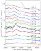 |
Fig. 4 Eleven spectra of SN 2013dx (various colors) and 1998bw (blue only) at comparable rest-frame phases, marked in days with respect to the explosion time of GRB130702A. As in Fig. 3, the SN 2013dx spectra have been smoothed and vertically shifted by 2 × 10-17 erg cm-2 s-1 Å-1, with the earliest one at the top and the latest one, not shifted, at the bottom. |
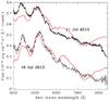 |
Fig. 5 Spectra of SN2013dx (black) taken on 11 and 16 July 2013, in rest-frame. For comparison, the models of the two available spectra of SN2010ah, taken at comparable phases after SN explosion, are shown in red. As in Fig. 3, the Jul. 11 spectrum has been vertically shifted by 3 × 10-17 erg cm-2 s-1 Å-1 with respect that of Jul. 16. |
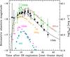 |
Fig. 6 Bolometric light curve of SN 2013dx (large circles) compared with those of other core-collapse type Ic SNe associated with a GRB or XRF (SNe 1998bw, crosses; 2003dh, triangles; 2006aj, squares; 2010bh, asterisks) and not associated with any detected high-energy event (SN1994I, small circles). Before day 20, several points of SN2013dx are affected by larger uncertainties than at later epochs, despite the higher brightness, because they are derived from the TNG photometry that is somewhat more noisy than the VLT photometry. The dashed line represents the model light curve for SN 2003dh, corresponding to the synthesis of 0.35 M⊙ of 56Ni, while the solid curve, which best reproduces the bolometric flux of SN 2013dx, was obtained by scaling down the above model curve by 25% and compressing it by 10%, which corresponds to a synthesized 56Ni mass of ~0.2 M⊙. |
4.4. Photospheric velocities
To estimate the velocity of the SN ejected material, we started out from the general similarity between our spectra and those of SN1998bw. Following Patat et al. (2001, see their Fig. 5), we identified the Si iiλ6355 feature and followed its redward shift along our spectra. In the spectra acquired between 17 and 22 July, the cosmological redshift and the blueshift due to the photospheric expansion combine to cause this absorption doublet to overlap with the telluric feature at 6870 Å. For these spectra, the position of the Si iiλ6355 cannot be measured.
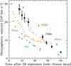 |
Fig. 7 Temporal evolution of the photosphere expansion velocity of SN 2013dx (large circles) measured directly on the spectra from the position of the minimum of the Si iiλ6355 absorption line. For comparison we report the photospheric velocities of other core-collapse Ic SNe (1994I, small circles; 2002ap, stars; 2003dh, triangles; 2006aj, small filled squares), as derived from spectral models (Sauer et al. 2006; Mazzali et al. 2002; 2003; b). For SN1998bw we report both the velocities derived from direct measurements (crosses, Patat et al. 2001) and those derived from models (large open squares, Nakamura et al. 2001). |
The time evolution of the photosphere expansion velocity as deduced from the minimum of the absorption trough of the Si iiλ6355 line is shown in Fig. 7 (large circles). The velocity decline extends from ~2.7 × 10⁴ km s-1 at 8 rest frame days from the explosion to ~3.5 × 10³ km s-1 at 40 days. Figure 7 also displays the photospheric velocities of other SNe, in particular that of SN 1998bw, computed by Patat et al. (2001) using the same procedure as that adopted by us. The photospheric velocities of SN 2013dx and SN 1998bw agree very well, although at very late time the latter retains a slightly higher velocity expansion (see also Fig. 4 of Patat et al. 2001). Comparing the expansion velocity of SN 2013dx with that of other SNe, we find that the former is higher than that of SN 1994D (Patat et al. 1996), SN 1994I (Millard et al. 1999), SN 1997ef (Patat et al. 2001) and SN 2006aj (Mazzali et al. 2006a,b), but not as extreme as that of SN 2003dh (Hjorth et al. 2003).
4.5. Physical parameters of SN 2013dx
The bolometric light curve of SN 2013dx shows that the peak luminosity of this SN is intermediate between those of the nearby GRB-SNe 1998bw and 2003dh on one hand and those of the two XRF-SNe 2006aj and 2010bh (Fig. 6) on the other. The spectrum of SN 2013dx is much more similar to that of the most energetic Ic SNe, and especially to SN 2010ah, which, among the broad-lined Ic SNe not accompanied by a GRB/XRF, is the most spectroscopically similar to SN 1998bw (Mazzali et al. 2013), although because of its lower ejecta mass, it has a significantly lower kinetic energy (1.2 × 1052 erg vs. 5 × 1052 erg inferred by Nakamura et al. 2001 for SN 1998bw).
The similarity of the light-curve shape of SN 2013dx to the shapes of those of SN 1998bw and SN 2003dh and the spectral resemblance to SN 1998bw and SN 2010ah led us to adopt these three previously known and well-studied SNe as “templates” for estimating the physical parameters of SN 2013dx through the relationships that link the SN ejecta mass Mej and kinetic energy EK to the observables, that is, to the width of the bolometric light curve and the photospheric velocities (Arnett 1982, see Sect. 4.1 in Mazzali et al. 2013). This method, described in detail by Mazzali et al. (2013; see also Valenti et al. 2008; Walker et al. 2014), should be applied with caution when only few SNe are available that provide a good match and the data coverage of both target and templates is not excellent. However, when the observational information is adequate, the outcome satisfactorily agrees with the results of modeling based on radiative transport: for SN 2010ah, which has a well-sampled light curve, but only two spectra taken around maximum light, the physical parameters obtained with the two approaches differ by no more than 25% (Mazzali et al. 2013).
The dataset presented here for SN 2013dx is detailed and rich, and we can compare it with as many as three template SNe with good data for which models were developed (Nakamura et al. 2001; Deng et al. 2005; Corsi et al. 2011; Mazzali et al. 2003; 2006a, 2013). This allows us to use the rescaling method to describe the physics of SN 2013dx with good accuracy. Developing a dedicated model is beyond the scope of this paper, but will be presented in the future.
Based on the similarity of the light-curve shape of SN2013dx and SN2003dh, we adapted the model curve of 2003dh (Mazzali et al. 2003; Deng et al. 2005) by compressing it by 10% in time and dimming it by 25% in flux. We thus obtained the synthetic curve reported in Fig. 6 (solid line). Since SN 2003dh produced an estimated 56Ni mass of ~0.35 M⊙ (Mazzali et al. 2006a), the 25% flux dimming corresponds to a 56Ni mass of 0.26 M⊙. However, this is further reduced by the effect of the 10% faster temporal evolution of SN 2013dx with respect to SN 2013dx. By taking this into account and assuming 56Ni decay dominates at early times (i.e., neglecting the contribution of 56Co decay), we obtain a further reduction of 20%, meaning that the final estimated 56Ni mass synthesized by SN 2013dx should be ~0.2 M⊙.
From a spectroscopic point of view, SN2013dx is a close analog of the GRB-SN prototype SN1998bw and a very close analog of the broad-lined type Ic SN2010ah, although in the latter case the comparison is limited to only two spectra. This suggests that the photospheric velocities are similar and that the kinetic energy of SN2013dx may then just simply scale like the ejecta mass.
Using the observed light curve width τ and measured photospheric velocities of SNe 1998bw, 2003dh, 2013dx (Figs. 6 and 7) and SN 2010ah (Mazzali et al. 2013), we applied the scaling relationships to SN2013dx and to each of the adopted template SN. Then we averaged the results and found for SN2013dx Mej = 7 ± 2 M⊙ and EK = (35 ± 10) × 1051 erg. Our errors on these physical quantities reflect conservatively the empirical nature of the method and its uncertainties (for instance, the fact that the phases at which the measured photospheric velocities are compared are never identical for the target and the template SN). The progenitor of SN 2013dx is thus probably 25–30 M⊙, which is 15–20% less massive than that estimated for SN 1998bw (30–35 M⊙, Maeda et al. 2006).
4.6. Field of SN2013dx
The field of SN 2013dx shows a bright galaxy southward of the transient, at ~8′′ from the SN position (see Fig. 8). This could have been the SN host, since the faint source (R = 23.01) at 0.6′′ from SN 2013dx was initially misclassified as a star in the SDSS (Singer et al. 2013). For this reason, Leloudas et al. (2013) obtained a spectrum of this galaxy, reporting a z = 0.145, which is the same as that of the transient (Mulchaey et al. 2013a,b; D’Avanzo et al. 2013c). Kelly et al. (2013) performed an extensive study of this galaxy and its outskirt, concluding that the SN 2013dx host galaxy is a dwarf satellite of the bright one.
Many more galaxies are present in the SN 2013dx field. Kelly et al. 2013 noted that many of them have an SDSS photometric redshift compatible with that of the host and the bright galaxy. In addition, they also pointed out that the SDSS spctroscopic galaxy survey targeted five galaxies brighter than 17.7 within 15′ from SN 2013dx, their redshift being close to z = 0.145.
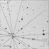 |
Fig. 8 Field of SN 2013dx with the slit positions used for FORS2 spectroscopy overimposed. Each slit position is identified by its observation date. Numbers mark the galaxies for which spectroscopic detection was secured. Red numbers refer to galaxies with redshift close to that of the SN 2013dx host galaxy (z = 0.145). Blue numbers refer to galaxies not related to the SN. The green “S” marks a field star included in the slit on 16 July. |
Observation dates, redshifts, and detected lines for the galaxies in the field of SN 2013dx.
We decided to use different slit position angles during our VLT spectroscopic campaign. This allowed us to study both the spectroscopic evolution of the SN and to determine the redshift of more nearby galaxies. The different position angles adopted are described in Table 5, and the corresponding slit orientations are displayed in Fig. 8. This figure also marks with numbers the 14 galaxies that we placed in the slit in our observations (“S” marks a star).
We determine the redshift of all these galaxies, although for three of them the determination is not completely certain because it relies on faint absorption or emission features. Table 6 illustrates the redshift of the galaxies, which are numbered as in Fig. 8. The uncertain redshifts are marked with “?”, while the last two columns of the table list the emission and absorption features on which the redshift determination is based. The spectra of our 14 field galaxies are shown in Appendix A.
It is interesting to note that 9 out of 14 galaxies lie within 0.03 from z = 0.145, that is, the redshift of SN 2013dx, and one more is within 0.2. These ten galaxies are marked in red in Fig. 8, while the remaining four are marked in blue. In particular, we confirm the photometric redshifts reported for two of the field galaxies in Fig. 2 of Kelly et al. (2013), their sources S3 and S5. This is clear evidence that SN 2013dx occurred in a group or a small cluster of galaxies. This conclusion is strengthened by the fact that many more galaxies in the SDSS, falling just outside the field of view of our images, have a spectroscopic or photometric redshift consistent with z = 0.145. In detail, since the angular separation among the two farthest galaxies with the same redshift in the field is ~3′, the physical extent of the group at z = 0.145 is ~600 kpc. This is the first SN associated with a long GRB detected in such an environment (and, to our knowledge, the first long GRB in general). For the SN 1998bw environment, a candidate cluster was first claimed (Duus & Newell 1977), but then not confirmed by spectroscopic analysis (Foley et al. 2006). For SN 2012bz, associated with GRB 120422A, two objects have been reported at the redshift of the GRB (Schulze et al. 2014). However, this looks like an interacting system consisting of two or possibly three galaxies, and not like a group.
Intuitively, one may argue that the probability of hosting a GRB should be higher in the largest galaxy of the cluster, where the maximum star-formation occurs. However, the dwarf galaxies have comparatively high or higher specific star-formation rates, which might bias the probability of hosting a GRB in their favor. Indeed, studies on complete samples of GRBs (see, e.g., Perley et al. 2015; Vergani et al. 2015) show that at z< 1 long GRBs strongly prefer low-mass galaxies (confirming previous studies on incomplete samples). This is probably because GRB progenitors are more easily developed in low-metallicity environments, which possess a high specific SFR.
5. Conclusions
We have presented an extensive and sensitive ground-based observational campaign on the SN associated with GRB 130702A at z = 0.145, one of the nearest GRB-SNe detected so far. Its relative proximity guaranteed the construction of a nice dataset with a good S/N. The properties of SN 2013dx are similar to those of previous GRB- and XRF-SNe: the peak luminosity is intermediate between those of GRB-SNe and XRF-SNe, and the photospheric velocities are more similar to those of GRB-SNe. Accordingly, the physical parameters of SN 2013dx, derived with the empirical method based on the rescaling of the quantities known for other SNe, are similar to those determined for the previous GRB-SNe, but somewhat lower than those of SN 1998bw: we estimate a synthesized 56Ni mass of ~0.2 M⊙, an ejecta mass of Mej ~ 7 M⊙, and a kinetic energy of EK ~ 35 × 1051 erg.
Furthermore, we performed a study of the SN 2013dx environment through spectroscopy of the field galaxies close to the host of GRB 130702A. We find that 65% of the observed targets have the same redshift as SN 2013dx, indicating that this is a group of galaxies. This represents the first report of a GRB-SN association taking place in a galaxy group or cluster.
Online material
Appendix A: SN 2013dx field galaxy spectra
In this appendix we report the 14 spectra of the galaxies in the field of SN 2013dx (see also Sect. 4.6).
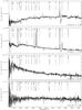 |
Fig. A.1 Spectra of the field galaxies of SN 2013dx. Wavelengths are in observer frame and galaxies are numbered as in Table 6 and Fig. 8. |
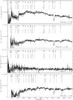 |
Fig. A.1 continued. |
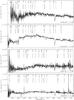 |
Fig. A.1 continued. |
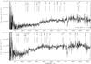 |
Fig. A.1 continued. |
Acknowledgments
We thank an anonymous referee for several helpful comments. We are grateful to the ESO Director for awarding Discretionary Time to this project. We thank S. Valenti for several helpful discussions and F. Patat for providing the photospheric velocities for SN 1998bw. We thank the TNG staff, in particular G. Andreuzzi, L. Di Fabrizio, and M. Pedani, for their valuable support with TNG observations, and the Paranal Science Operations Team, in particular H. Boffin, S. Brillant, C. Cid, O. Gonzales, V. D. Ivanov, D. Jones, J. Pritchard, M. Rodrigues, L. Schmidtobreick, F. J. Selman, J. Smoker and S. Vega. The Dark Cosmology Centre is funded by the Danish National Research Foundation. V.D.E. acknowledges partial support from PRIN MIUR 2009. This research was partially supported by INAF PRIN 2011, PRIN MIUR 2010/2011, and ASI-INAF grants I/088/06/0 and I/004/11/1. F.B. acknowledges support from FONDECYT through Postdoctoral grant 3120227 and from Project IC120009 “Millennium Institute of Astrophysics (MAS)” of the Iniciativa Cientifica Milenio del Ministerio de Economia, Fomento y Turismo de Chile. D.M. acknowledges the Instrument Center for Danish Astrophysics for support. The spectra are publicly available on WISeREP – http://wiserep.weizmann.ac.il
References
- Arnett, W. D. 1982, ApJ, 253, 785 [NASA ADS] [CrossRef] [Google Scholar]
- Berger, E., Chornock, R., Holmes, T. R., et al. 2011, ApJ, 743, 204 [NASA ADS] [CrossRef] [Google Scholar]
- Bersier, D., Fruchter, A. S., Strolger, L.-G., et al. 2006, ApJ, 643, 284 [NASA ADS] [CrossRef] [Google Scholar]
- Bloom, J. S., Kulkarni, S. R., Djorgovski, S. G., et al. 1999, Nature, 401, 453 [NASA ADS] [CrossRef] [Google Scholar]
- Bromberg, O., Granot, J., Lyubarsky, Y., & Piran, T. 2014, MNRAS, 443, 1532 [NASA ADS] [CrossRef] [Google Scholar]
- Bufano, F., Pian, E., Sollerman, J., et al. 2012, ApJ, 753, 67 [NASA ADS] [CrossRef] [Google Scholar]
- Campana, S., Mangano, V., Blustin, A. J., et al. 2006, Nature, 442, 1008 [NASA ADS] [CrossRef] [PubMed] [Google Scholar]
- Cano, Z., Bersier, D., Guidorzi, C., et al. 2011a, ApJ, 740, 41 [NASA ADS] [CrossRef] [Google Scholar]
- Cano, Z., Bersier, D., Guidorzi, C., et al. 2011b, MNRAS, 413, 669 [NASA ADS] [CrossRef] [Google Scholar]
- Cano, Z., de Ugarte Postigo, A., Pozanenko, A., et al. 2014, A&A, 568, A19 [NASA ADS] [CrossRef] [EDP Sciences] [Google Scholar]
- Cenko, S. B., Gal Yam, A., Kasliwal, M. M., et al. 2013, GCN Circ., 14998, 1 [NASA ADS] [Google Scholar]
- Cheung, T., Vianello, G., Zhu, S., et al. 2013, GCN Circ., 14971, 1 [NASA ADS] [Google Scholar]
- Chincarini, G., Zerbi, F. M., Antonelli, A., et al. 2003, The Messenger 113, 40 [NASA ADS] [Google Scholar]
- Cobb, B. E., Bloom, J. S., Perley, D. A., et al. 2010, ApJ, 718, 150 [Google Scholar]
- Collazzi, A. C., & Connaughton, V. 2013, GCN Circ., 14972, 1 [NASA ADS] [Google Scholar]
- Corsi, A., Ofek, E. O., Frail, D. A., et al. 2011, ApJ, 741, 76 [NASA ADS] [CrossRef] [Google Scholar]
- Covino, S., Stefanon, M., Fernandez-Soto, A., et al. 2004, SPIE, 5492, 1613 [Google Scholar]
- Crowther, P. A. 2007, ARA&A, 45, 177 [NASA ADS] [CrossRef] [Google Scholar]
- D’Avanzo, P., Porterfield, B., Burrows, D. N., et al. 2013a, GCN Circ., 14973, 1 [NASA ADS] [Google Scholar]
- D’Avanzo, P., Melandri, A., & Evans, P. A. 2013b, GCN Circ., 14982, 1 [NASA ADS] [Google Scholar]
- D’Avanzo, P., Melandri, A., Andreuzzi, G., & Mainella, G., et al. 2013c, GCN Circ., 14977, 1 [NASA ADS] [Google Scholar]
- D’Avanzo, P., D’Elia, V., Tagliarri, G., et al. 2013d, GCN Circ., 14984, 1 [NASA ADS] [Google Scholar]
- D’Elia, V., D’Avanzo, P., Melandri, A., et al. 2013a, GCN Circ., 15000, 1 [NASA ADS] [Google Scholar]
- D’Elia, V., D’Avanzo, P., Melandri, A., et al. 2013b, CBET, 3587, 1 [NASA ADS] [Google Scholar]
- Della Valle, M., Malesani, D., Benetti, S., et al. 2003, A&A, 406, L33 [NASA ADS] [CrossRef] [EDP Sciences] [Google Scholar]
- Della Valle, M., Chincarini, G., Panagia, N., et al. 2006a, Nature, 444, 1050 [NASA ADS] [CrossRef] [PubMed] [Google Scholar]
- Della Valle, M., Malesani, D., Bloom, J. S., et al. 2006b, ApJ, 642, L103 [NASA ADS] [CrossRef] [Google Scholar]
- Deng, J., Tominaga, N., Mazzali, P. A., et al. 2005, ApJ, 624, 898 [NASA ADS] [CrossRef] [Google Scholar]
- Duus, A., & Newell, B. 1977, ApJS, 35, 209 [NASA ADS] [CrossRef] [Google Scholar]
- Ferrero, P., Kann, D. A., Zeh, A., et al. 2006, A&A, 457, 857 [NASA ADS] [CrossRef] [EDP Sciences] [Google Scholar]
- Foley, S., Watson, D., Gorosabel, J., et al. 2006, A&A, 447, 891 [NASA ADS] [CrossRef] [EDP Sciences] [Google Scholar]
- Fryer, C. L., Brown, P. J., Bufano, F., et al. 2009, ApJ, 707, 193 [NASA ADS] [CrossRef] [Google Scholar]
- Galama, T. J., Vreeswijk, P. M., van Paradijs, J., et al. 1998, Nature, 395, 670 [NASA ADS] [CrossRef] [Google Scholar]
- Garnavich, P., Stanek, K. Z., Wyrzykowski, L., et al. 2003, ApJ, 582, 924 [NASA ADS] [CrossRef] [Google Scholar]
- Golenetskii, S., Aptekar, R., Pal’Shin, V., et al. 2013, GCN Circ., 14986, 1 [NASA ADS] [Google Scholar]
- Gorosabel, J., Fynbo, J. P. U., Fruchter, A., et al. 2005, A&A, 437, 411 [NASA ADS] [CrossRef] [EDP Sciences] [Google Scholar]
- Greiner, J., Klose, S., Salvato, M., et al. 2003, ApJ, 599, 1223 [NASA ADS] [CrossRef] [Google Scholar]
- Guidorzi, C., Mundell, C. G., Steele, I. A., & Singer, L. P. 2013, GCN Circ., 14968, 1 [NASA ADS] [Google Scholar]
- Hjorth, J., & Bloom, J. S. 2012, in Gamma-Ray Bursts, eds. C. Kouveliotou, R. A. M. J. Wijers, & S. E. Woosley (Cambridge: Cambridge Univ. Press) [Google Scholar]
- Hjorth, J., Sollerman, J., Møller, P., et al. 2003, Nature, 423, 847 [NASA ADS] [CrossRef] [PubMed] [Google Scholar]
- Hurley, K., Goldsten, J., Connaughton, V., et al. 2013, GCN Circ., 14974, 1 [NASA ADS] [Google Scholar]
- Jin, Z.-P., Covino, S., Della Valle, M., et al. 2013, ApJ, 774, 114 [NASA ADS] [CrossRef] [Google Scholar]
- Kelly, P. L., Filippenko, A. V., Fox, O. D., Zheng, W., & Clubb, K. I. 2013, ApJ, 775, L5 [NASA ADS] [CrossRef] [Google Scholar]
- Kinney, A., Calzetti, D., Bohlin, R. C., et al. 1996, ApJ, 467, 38 [NASA ADS] [CrossRef] [Google Scholar]
- Lazzati, D., Covino, S., Ghisellini, G., et al. 2001, A&A, 378, 996 [NASA ADS] [CrossRef] [EDP Sciences] [Google Scholar]
- Leloudas, G., Fynbo, J. P. U., Schulze, S., et al. 2013, GCN Circ., 14983, 1 [NASA ADS] [Google Scholar]
- Levesque, E. M. 2014, PASP, 126, 1 [NASA ADS] [CrossRef] [Google Scholar]
- Lyutikov, M. 2011, MNRAS, 411, 2054 [NASA ADS] [CrossRef] [Google Scholar]
- Maeda, K., Nomoto, K., Mazzali, P. A., & Deng, J. 2006, ApJ, 640, 854 [NASA ADS] [CrossRef] [Google Scholar]
- Malesani, D., Tagliaferri, G., Chincarini, G., et al. 2004, ApJ, 609, L5 [NASA ADS] [CrossRef] [Google Scholar]
- Masetti, N., Palazzi, E., Pian, E., et al. 2003, A&A, 404, 465 [NASA ADS] [CrossRef] [EDP Sciences] [Google Scholar]
- Mazzali, P. A., Deng, J., Maeda, K., et al. 2002, ApJ, 572, L61 [NASA ADS] [CrossRef] [Google Scholar]
- Mazzali, P. A., Deng, J., Tominaga, N., et al. 2003, ApJ, 599, 95 [Google Scholar]
- Mazzali, P. A., Deng, J., Pian, E., et al. 2006a, ApJ, 645, 1323 [NASA ADS] [CrossRef] [Google Scholar]
- Mazzali, P. A., Deng, J., Nomoto, K., et al. 2006b, Nature, 442, 1018 [NASA ADS] [CrossRef] [PubMed] [Google Scholar]
- Mazzali, P. A., Walker, E. S., Pian, E., et al. 2013, MNRAS, 432, 2463 [NASA ADS] [CrossRef] [Google Scholar]
- Mazzali, P. A., McFadyen, A. I., Woosley, S. E., Pian, E., & Tanaka, M. 2014, MNRAS, 443, 67 [NASA ADS] [CrossRef] [Google Scholar]
- Melandri, A., Pian, E., Ferrero, P., et al. 2012, A&A, 547, A82 [NASA ADS] [CrossRef] [EDP Sciences] [Google Scholar]
- Melandri, A., Pian, E., D’Elia, V., et al. 2014, A&A, 565, A72 [NASA ADS] [CrossRef] [EDP Sciences] [Google Scholar]
- Millard, J., Branch, D., Baron, E., et al. 1999, ApJ, 527, 746 [NASA ADS] [CrossRef] [Google Scholar]
- Modjaz, M., Stanek, K. Z., Garnavich, P. M., et al. 2006, ApJ, 645, L21 [NASA ADS] [CrossRef] [Google Scholar]
- Mulchaey, J., Kasliwal, M. M., Arcavi, I., Bellm, E., & Kelson, D. 2013a, ATel 5191, 1 [Google Scholar]
- Mulchaey, J., Kasliwal, M. M., Arcavi, I., Bellm, E., & Kelson, D. 2013b, GCN Circ., 14985, 1 [NASA ADS] [Google Scholar]
- Nakamura, T., Mazzali, P. A., Nomoto, K., et al. 2001, ApJ, 550, 991 [NASA ADS] [CrossRef] [Google Scholar]
- Patat, F., Benetti, S., Cappellaro, E., et al. 1996, MNRAS, 278, 111 [NASA ADS] [CrossRef] [Google Scholar]
- Patat, F., Cappellaro, E., Danziger, J., et al. 2001, ApJ, 555, 900 [NASA ADS] [CrossRef] [Google Scholar]
- Perley, D., & Kasliwal, M. 2014, GCN Circ., 14979, 1 [Google Scholar]
- Perley, D., Perley, R. A., Hjorth, J., et al. 2015, ApJ, 801, 102 [NASA ADS] [CrossRef] [Google Scholar]
- Pian, E., Mazzali, P. A., Masetti, N., et al. 2006, Nature, 442, 1011 [NASA ADS] [CrossRef] [PubMed] [Google Scholar]
- Podsiadlowski, P., Ivanova, N., Justham, S., & Rappaport, S. 2010, MNRAS, 406, 840 [NASA ADS] [Google Scholar]
- Richmond, M. W., van Dyk, S. D., Ho, W., et al. 1996, AJ, 111, 327 [NASA ADS] [CrossRef] [Google Scholar]
- Sauer, D., Mazzali, P. A., Deng, J., et al. 2006, MNRAS, 369, 1939 [NASA ADS] [CrossRef] [Google Scholar]
- Schlegel, D. J., Finkbeiner, D. P., & Davis, M. 1998, ApJ, 500, 525 [NASA ADS] [CrossRef] [Google Scholar]
- Schulze, S., Lelloudas, G., Xu, D., et al. 2013a, GCN Circ., 14994, 1 [NASA ADS] [Google Scholar]
- Schulze, S., Lelloudas, G., Xu, D., et al. 2013b, CBET, 3587, 1 [NASA ADS] [Google Scholar]
- Schulze, S., Malesani, D., Cucchiara, A., et al. 2014, A&A, 566, A102 [NASA ADS] [CrossRef] [EDP Sciences] [Google Scholar]
- Singer, L. P., Cenko, S. B., Kasliwal, M. M., et al. 2013, ApJ, 776, L34 [NASA ADS] [CrossRef] [Google Scholar]
- Soderberg, A. M., Kulkarni, S. R., Fox, D. B., et al. 2005, ApJ, 627, 877 [NASA ADS] [CrossRef] [Google Scholar]
- Soderberg, A. M., Kulkarni, S. R., Price, P. A., et al. 2006, ApJ, 636, 391 [NASA ADS] [CrossRef] [Google Scholar]
- Soderberg, A. M., Nakar, E., Cenko, S. B., et al. 2007, ApJ, 661, 982 [NASA ADS] [CrossRef] [Google Scholar]
- Sparre, M., Sollerman, J., Fynbo, J. P. U., et al. 2011, ApJ, 735, 24 [Google Scholar]
- Stanek, K. Z., Matheson, T., Garnavich, P. M., et al. 2003, ApJ, 591, L17 [NASA ADS] [CrossRef] [Google Scholar]
- Tanvir, N. R., Rol, E., Levan, A. J., et al. 2010, ApJ, 725, 625 [NASA ADS] [CrossRef] [Google Scholar]
- Uzdensky, D. A., & MacFadyen, A. I. 2006, ApJ, 647, 1192 [NASA ADS] [CrossRef] [Google Scholar]
- Valenti, S., Benetti, S., Cappellaro, E., et al. 2008, MNRAS, 383, 1485 [NASA ADS] [CrossRef] [Google Scholar]
- van der Horst, A. J. 2013, GCN Circ., 14987, 1 [NASA ADS] [Google Scholar]
- Vergani, S. D., Salvaterra, R., Japelj, J., et al. 2015, A&A, submitted, [arXiv:1409.7064] [Google Scholar]
- Walker, E. S., Mazzali, P. A., Pian, E., et al. 2014, MNRAS, 442, 2768 [NASA ADS] [CrossRef] [Google Scholar]
- Woosley, S. E., & Bloom, J. S. 2006, ARA&A, 44, 507 [NASA ADS] [CrossRef] [Google Scholar]
- Woosley, S. E., & Heger, A. 2012, ApJ, 753, 32 [NASA ADS] [CrossRef] [Google Scholar]
- Xu, D., Esamdin, A., Ma, L., & Zhang, X. 2013a, GCN Circ., 14975, 1 [NASA ADS] [Google Scholar]
- Xu, D., de Ugarte Postigo, A., Leloudas, G., et al. 2013b, ApJ, 776, 98 [NASA ADS] [CrossRef] [Google Scholar]
- Zeh, A., Klose, S., & Hartmann, D. H. 2004, ApJ, 609, 952 [NASA ADS] [CrossRef] [Google Scholar]
- Zerbi, F. M., Chincarini, G., Ghisellini, G., et al. 2001, Astron. Nachr., 322, 275 [NASA ADS] [CrossRef] [Google Scholar]
- Zhang, B., & Mészáros, P. 2004, IJMPA, 19, 2385 [Google Scholar]
- Zhang, W., Woosley, S. E., & MacFadyen, A. I. 2003, ApJ, 586, 356 [NASA ADS] [CrossRef] [Google Scholar]
All Tables
Observation dates, redshifts, and detected lines for the galaxies in the field of SN 2013dx.
All Figures
|
Fig. 1 SN 2013dx field acquired with VLT/FORS2 on July 27 in the R band. The SN and host galaxy position is indicated by two perpendicular markers. Two companion galaxies are clearly visible southward. |
| In the text | |
|
Fig. 2 GRB 130702A/SN2013dx optical and near-infrared light curves. The time origin t = 0 coincides with the GRB explosion time. |
| In the text | |
|
Fig. 3 Sixteen dereddened, host- and afterglow-subtracted TNG and VLT spectra. For clarity, the spectra have been vertically shifted by 2 × 10-17 erg cm-2 s-1 Å-1, with the earliest one (TNG, Jul. 9) at top and the latest one, not shifted, at the bottom. All VLT spectra are smoothed with a boxcar of 8 Å, with the exception of those from Jul. 20 and 22 (that have the lowest S/N), which are smoothed by 25 Å. All TNG spectra are smoothed with a boxcar of 7 Å. The time intervals are computed from the GRB explosion time. Black filled circles mark the position of the SiII6355 feature, used to determine the photospheric velocity of the ejecta (see Sect. 4.4). |
| In the text | |
|
Fig. 4 Eleven spectra of SN 2013dx (various colors) and 1998bw (blue only) at comparable rest-frame phases, marked in days with respect to the explosion time of GRB130702A. As in Fig. 3, the SN 2013dx spectra have been smoothed and vertically shifted by 2 × 10-17 erg cm-2 s-1 Å-1, with the earliest one at the top and the latest one, not shifted, at the bottom. |
| In the text | |
|
Fig. 5 Spectra of SN2013dx (black) taken on 11 and 16 July 2013, in rest-frame. For comparison, the models of the two available spectra of SN2010ah, taken at comparable phases after SN explosion, are shown in red. As in Fig. 3, the Jul. 11 spectrum has been vertically shifted by 3 × 10-17 erg cm-2 s-1 Å-1 with respect that of Jul. 16. |
| In the text | |
|
Fig. 6 Bolometric light curve of SN 2013dx (large circles) compared with those of other core-collapse type Ic SNe associated with a GRB or XRF (SNe 1998bw, crosses; 2003dh, triangles; 2006aj, squares; 2010bh, asterisks) and not associated with any detected high-energy event (SN1994I, small circles). Before day 20, several points of SN2013dx are affected by larger uncertainties than at later epochs, despite the higher brightness, because they are derived from the TNG photometry that is somewhat more noisy than the VLT photometry. The dashed line represents the model light curve for SN 2003dh, corresponding to the synthesis of 0.35 M⊙ of 56Ni, while the solid curve, which best reproduces the bolometric flux of SN 2013dx, was obtained by scaling down the above model curve by 25% and compressing it by 10%, which corresponds to a synthesized 56Ni mass of ~0.2 M⊙. |
| In the text | |
|
Fig. 7 Temporal evolution of the photosphere expansion velocity of SN 2013dx (large circles) measured directly on the spectra from the position of the minimum of the Si iiλ6355 absorption line. For comparison we report the photospheric velocities of other core-collapse Ic SNe (1994I, small circles; 2002ap, stars; 2003dh, triangles; 2006aj, small filled squares), as derived from spectral models (Sauer et al. 2006; Mazzali et al. 2002; 2003; b). For SN1998bw we report both the velocities derived from direct measurements (crosses, Patat et al. 2001) and those derived from models (large open squares, Nakamura et al. 2001). |
| In the text | |
|
Fig. 8 Field of SN 2013dx with the slit positions used for FORS2 spectroscopy overimposed. Each slit position is identified by its observation date. Numbers mark the galaxies for which spectroscopic detection was secured. Red numbers refer to galaxies with redshift close to that of the SN 2013dx host galaxy (z = 0.145). Blue numbers refer to galaxies not related to the SN. The green “S” marks a field star included in the slit on 16 July. |
| In the text | |
|
Fig. A.1 Spectra of the field galaxies of SN 2013dx. Wavelengths are in observer frame and galaxies are numbered as in Table 6 and Fig. 8. |
| In the text | |
|
Fig. A.1 continued. |
| In the text | |
|
Fig. A.1 continued. |
| In the text | |
|
Fig. A.1 continued. |
| In the text | |
Current usage metrics show cumulative count of Article Views (full-text article views including HTML views, PDF and ePub downloads, according to the available data) and Abstracts Views on Vision4Press platform.
Data correspond to usage on the plateform after 2015. The current usage metrics is available 48-96 hours after online publication and is updated daily on week days.
Initial download of the metrics may take a while.