| Issue |
A&A
Volume 577, May 2015
|
|
|---|---|---|
| Article Number | A124 | |
| Number of page(s) | 11 | |
| Section | The Sun | |
| DOI | https://doi.org/10.1051/0004-6361/201425309 | |
| Published online | 13 May 2015 | |
Stopping frequency of type III solar radio bursts in expanding magnetic flux tubes
SUPA School of Physics and Astronomy, University of Glasgow, Glasgow, G12 8QQ, UK
e-mail: This email address is being protected from spambots. You need JavaScript enabled to view it.
Received: 10 November 2014
Accepted: 10 March 2015
Abstract
Aims. Understanding the properties of type III radio bursts in the solar corona and interplanetary space is one of the best ways to remotely deduce the characteristics of solar accelerated electron beams and the solar wind plasma. One feature of all type III bursts is the lowest frequency they reach (or stopping frequency). This feature reflects the distance from the Sun that an electron beam can drive the observable plasma emission mechanism. The stopping frequency has never been systematically studied before from a theoretical perspective.
Methods. Using numerical kinetic simulations, we explore the different parameters that dictate how far an electron beam can travel before it stops inducing a significant level of Langmuir waves, responsible for plasma radio emission. We use the quasilinear approach to model the resonant interaction between electrons and Langmuir waves self-consistently in inhomogeneous plasma, and take into consideration the expansion of the guiding magnetic flux tube and the turbulent density of the interplanetary medium.
Results. We find that the rate of radial expansion has a significant effect on the distance an electron beam travels before enhanced levels of Langmuir waves, hence radio waves, cease. Radial expansion of the guiding magnetic flux tube rarefies the electron stream to the extent that the density of non-thermal electrons is too low to drive Langmuir wave production. The initial conditions of the electron beam have a significant effect, where decreasing the beam density or increasing the spectral index of injected electrons would cause higher type III stopping frequencies. We also demonstrate how the intensity of large-scale density fluctuations increases the highest frequency to which Langmuir waves can be driven by the beam and how the magnetic field geometry can be the cause of type III bursts that are only observed at high coronal frequencies.
Key words: Sun: flares / Sun: radio radiation / Sun: particle emission / solar wind / Sun: corona / Sun: magnetic fields
© ESO, 2015
1. Introduction
Type III radio bursts observed in the metre range were initially classified (Wild & McCready 1950) as an impulsive radio frequency signal that drifted from high to low frequencies with time. They were given the name “type III” because the rate at which they drift in frequency with time (or drift rate) was higher than “type I” and “type II” bursts. Type III bursts are one of the most frequently observed impulsive electromagnetic signals driven by the Sun and are produced by accelerated electrons beams travelling at near-relativistic energies through the plasma of the solar system (see e.g. Goldman 1983; Suzuki & Dulk 1985; Dulk 1985; Melrose 1990; Muschietti 1990; Reid & Ratcliffe 2014, for reviews). Understanding which properties of accelerated electron beams and the solar wind plasma give rise to certain features in type IIIs allows us to use these transient burst properties as a diagnostic tool.
The escaping radio emission responsible for type III bursts can be broadly described as a two-stage process (first suggested by Ginzburg & Zhelezniakov 1958). The first stage is a two-stream instability between the electron beam and the background plasma that induces a high level of Langmuir waves. The second stage is wave-wave interactions between Langmuir waves and either ion-sound waves for fundamental emission or oppositely propagating Langmuir waves for harmonic emission. The current theory has been refined by many authors (e.g. Zheleznyakov & Zaitsev 1970; Smith 1970; Zaitsev et al. 1972; Smith et al. 1976; Melrose 1980b, 1987; Goldman 1983; Dulk 1985; Kontar et al. 1998; Mel’Nik 2003; Ledenev et al. 2004) and continues to develop with the advent of numerical simulations (e.g. Takakura & Shibahashi 1976; Magelssen & Smith 1977; Grognard 1985; Robinson 1992; Kontar 2001c; Li et al. 2008; Kontar & Reid 2009; Tsiklauri 2010, 2011; Reid & Kontar 2013; Ratcliffe et al. 2012; Li & Cairns 2014; Ratcliffe & Kontar 2014).
Type III bursts cover a wide range of frequencies. The starting frequency of type III bursts varies from hundreds of MHz, and rarely GHz, down to 1 MHz and below. The stopping frequency of type III bursts varies over a even wider frequency range from the hundreds to tens of MHz for type III bursts that originate only in the corona, all the way down to tens of kHz for type III bursts from interplanetary space. The properties of an electron beam and the background heliospheric plasma govern at what frequencies the type III radio emission starts and stops being observed. Whilst recent studies have investigated what is important in determining the starting frequency of type III bursts (Reid et al. 2011, 2014), the processes affecting the stopping frequency of type III bursts has never been systematically investigated. Figure 1 shows an example of many type III bursts observed before and after a large flare. Although electron beams associated with the flare reached frequencies around 0.04 MHz, the majority of other type III bursts stopped at higher frequencies. What plasma parameters dictate at what frequency a type III burst stops is unclear.
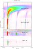 |
Fig. 1 Example of many type III bursts on 16 February 2014, detected by the WAVES instrument on the WIND spacecraft at 14−0.02 MHz (Bougeret et al. 1995), the Nançay Decametre Array at 80−14 MHz (Lecacheux 2000) and Phoenix 4 at 900−200 MHz (Benz et al. 2009). The large type III burst at 09:30 was associated with a GOES M1 flare. We can observe type III bursts stopping at a variety of different frequencies. The periodicity observed below 1 MHz is an artefact. |
Previous observational studies of type III burst stopping frequencies by Leblanc et al. (1995, 1996) used radio data from the WAVES instrument onboard the WIND spacecraft and the URAP experiment on the Ulysses spacecraft (Stone et al. 1992). They analysed type III bursts detected only by Ulysses between 1990 and 1994 (Leblanc et al. 1995) and by both WIND and Ulysses detected below 1 MHz between 1994 and 1995 (Leblanc et al. 1996). Each type III burst was given a stopping frequency, estimated from the lowest observable frequency on the type III dynamic spectra. Repeating the process a number of times for the same type III bursts, they estimated an error on their results of 12%. Typical stopping frequencies for type III bursts were observed between 100−200 kHz for weak type III bursts and 20−50 kHz for strong type III bursts. Neither study observed type III bursts below 9 kHz despite the plasma frequency at Ulysses being as low as 3 kHz during observations. They found a connection between the intensity of the type III burst emission and the stopping frequency. The higher the intensity of the type III burst, the lower the stopping frequency tended to be.
There were three postulations by Leblanc et al. (1995) for what influences the burst’s stopping frequency. In the first, the electron beam is diluted by expansion of the guiding magnetic flux tube. The diluted electron beam becomes ineffective in forming the required magnitude of the positive slope in velocity space for generating Langmuir waves. In the second, the level of density fluctuations or ion-acoustic waves required to convert Langmuir waves into electromagnetic waves decreases as a function of distance from the Sun and throttles the production of radio emission (previously suggested by de Genouillac & Escande 1981). In the third, the density fluctuations suppress the level of Langmuir waves excited by the electron beam (e.g. Nishikawa & Ryutov 1976) and thus cease the production of radio emission. That large scale density fluctuations suppress Langmuir wave growth has been discussed at length by many authors (e.g. Smith & Sime 1979; Muschietti et al. 1985; Kontar 2001b; Reid & Kontar 2010; Li et al. 2011; Ratcliffe et al. 2012).
Dulk et al. (1996) tested the hypothesis that radio wave prorogation governs the lowest type III frequencies and that the cut-offs are not intrinsic to the radiation mechanism. Using simultaneous WIND and Ulysses (which was behind the Sun) observations, they found a reasonable correlation coefficient of 0.51 but with a high degree of scatter. 28% of bursts they observed had the same stopping frequency to within a factor of 1.12, whilst 50% of the bursts had the same stopping frequency to within a factor of 1.4. At the extremes, the stopping frequency of type III bursts differed by a factor of 5. The difference in cutoff frequencies suggests that some directivity or rather the blocking of radio emission between source and observer by density fluctuations can play a role in determining stopping frequency. However, it is not the dominant process because the stopping frequency of type III bursts can vary over many orders of magnitude in frequency. For example in the study by Dulk et al. (1996) they recorded stopping frequencies from 300 kHz down to 20 kHz. The large spread suggests that the plasma processes involved with the production of type III bursts largely determine the stopping frequency.
A more recent study using the WAVES instrument (Bougeret et al. 2008) onboard the STEREO spacecraft was carried out by Krupar et al. (2014) on 154 type III bursts occurred between 2007 and 2013. They found that the stopping frequency in 65% to 75% of events was at 125 kHz, the lowest frequency channel measured. It is also important to mention that the measured stopping frequency is dependent upon the sensitivity of the radio receiver and/or the level of ambient signal from the background plasma and the galactic background.
The necessary condition for a type III radio burst is a population of coronal accelerated electrons that are able to drive Langmuir waves with access to open magnetic field lines. If a population of accelerated electrons is able to drive Langmuir wave generation, what causes this Langmuir wave generation to cease and how does it vary with distance from the Sun? To answer these questions, we have simulated the outward propagation of a solar electron beam injected in the low corona. We self-consistently modelled the wave-particle interactions that govern the production of Langmuir waves through the beam-plasma instability. We also modelled collisional effects, wave refraction in an inhomogeneous background plasma, the expanding magnetic field lines of the solar corona and solar wind. The model and the initial condition of the injected electron beam are all described in Sect. 2. Using Langmuir wave energy density as a proxy for the level of radio emission generated by an electron beam, we considered a number of different effects that govern when the production of Langmuir waves will cease: the expansion of guiding magnetic flux tube in Sect. 3, the level of density fluctuations in Sect. 4, and the initial beam parameters in Sect. 5. Our results are discussed in Sect. 6.
2. Model equations, initial conditions, and approximations
2.1. Model
To predict the evolution of an electron beam travelling through the heliosphere we will rely on the quasilinear approximation of wave-particle interactions (e.g. Drummond & Pines 1962; Vedenov et al. 1962). This utilises the WKB approximation where we are treating waves as quasi-particles interacting resonantly ωpe(r) = kv, where ωpe(r) is the background plasma angular frequency (Bian et al. 2014). Using f(v,r,t) as the electron distribution function and W(v,r,t) as the Langmuir wave spectral energy density in the one dimension of propagation, we can describe the time evolution using  where
where  is the Langmuir wave dispersion relation, me is the electron mass, e is the electron charge, ne(r) is the background plasma density (defined in Sect. 2.2.2) and lnΛ is the Coulomb logarithm that is assumed constant and =20. M(r) is the cross-sectional area of the magnetic flux tube (defined in Sect. 3. In this case where M(r) ∝ r2 it corresponds to spherically symmetric expansion of the flux tube (e.g. Reid & Kontar 2013). For the background electron thermal velocity we have
  where kB is the Boltzmann constant. The background plasma frequency is defined as
  .
.
For the particles, the physical processes we are considering in order of terms from left to right in Eq. (1) are: change in time of the distribution function, transport through space in an expanding magnetic field, resonant interaction with Langmuir waves, collisional damping from the background plasma, and a source term of electrons S(v,r,t) is defined in Sect. 2.2.1.
For the Langmuir waves, the physical processes we are considering in order of terms from left to right in Eq. (2) are: change in time of the Langmuir wave spectral energy density, propagation of waves through space1, Langmuir wave refraction, resonant interaction with the high velocity electrons, Landau damping from the background Maxwellian plasma  , collisional damping from background ions
  , and the spontaneous generation from the background plasma.
2.2. Initial conditions
2.2.1. Electron beam
We introduce a source of electrons into the simulations, where the source function takes the following form:  (3)Each dimension of the source function is characterised by one parameter. The velocity distribution is given by
  (4)where α is the velocity spectral index. We have chosen α to be 7 that corresponds to 3.5 in energy space, and is indicative of injected electron beam spectral indices derived from X-ray observations during flares (e.g. Dennis 1988; Holman et al. 2011). The velocity normalisation constant is given by
  . The parameter nbeam is the total density of electrons injected at the centre of the injection site between the minimum and maximum velocities vmin = 2.6vTe = 1.43 × 109 cm s-1 and vmax = 36vTe = 2 × 1010 cm s-1. We set nbeam = 2 × 106 cm-3.
The spatial distribution is given by  (5)where the characteristic parameter in space is given by the spread of the electron beam d. We have chosen d at 109 cm which is a typical size of a flare acceleration region derived from simultaneous X-ray and radio observations (Reid et al. 2011, 2014). The centre of the injection, r = 0 has an altitude of rinj = 50 Mm, consistent with the estimates from a number of flares (Reid et al. 2011, 2014). This altitude corresponds to a density of 2.14 × 109 cm-3 and plasma frequency of 415 MHz in our density model (Sect. 2.2.2). Whilst we are injecting quite a large number of electrons into the simulation (nbeam/ne = 10-3), we note that the large background density will cause the majority of the electrons to lose their energy before they can escape the corona (Reid & Kontar 2013).
The temporal profile is given by  (6)where the characteristic parameter in time is given by the injection time τ. We have chosen τ = 0.001 s, which is equivalent to an instantaneous injection of electrons in the corona. The time normalisation constant is given by
  such that
  . An instantaneous injection was chosen to minimise the influence of injection time on the starting height that Langmuir waves are induced by the electron beam (Reid & Kontar 2013; Ratcliffe et al. 2014). The constant tinj = 4τ is a delay time such that four characteristic times can occur before the injection maximum.
2.2.2. Background plasma
We introduce a population of thermal electrons as a background plasma. This background Maxwellian population is characterised by a background temperature Te = 2 MK that corresponds to a background thermal velocity of vTe = 5.5 × 108 cm s-1. The choice of 2 MK is related to the higher Landau damping that is predicted from the strahl present in the heliosphere (e.g. Maksimovic et al. 2005).
For the background electron density ne(r), we use the density profile of the Parker model that solves the equations for a stationary spherical symmetric solution (Parker 1958) with normalisation factor found from satellites (Mann et al. 1999). 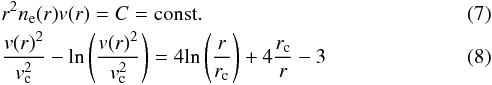 where the critical velocity vc is defined such that
  and the critical radius is defined by
  (both independent on r). Tsw is the temperature of the solar wind2, taken as 1 MK, Ms is the mass of the Sun, mp is the proton mass and
  is the mean molecular weight. The constant appearing above is fixed by satellite measurements near the Earth’s orbit (at r = 1 AU, n = 6.59 cm-3) and equates to 6.3 × 1034 s-1. This model is static in time, set at the start of the simulations. We justify this because the electron beam is moving at least two orders of magnitude faster than the solar wind velocity.
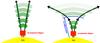 |
Fig. 2 Cartoon of an electron cloud (green) travelling upwards from an acceleration region through the corona, following the magnetic field. The density of the electron cloud is represented through the transparency. Left: an example of a constant radial expansion described by Eq. (12). Right: at a critical height rc the magnetic field lines begin to expand at an increased rate described by Eq. (13), causing the density of the electron cloud to decrease faster. |
We also consider a thermal level of Langmuir waves in the background plasma (e.g. Hannah et al. 2009, 2013; Reid & Kontar 2013) when wave collisions are weak. This takes the form 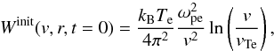 (9)where kB is the Boltzmann constant.
2.3. Langmuir wave energy density
Using the model and the initial conditions described in Sects. 2.1 and 2.2 respectively, we have simulated the propagation of an electron beam injected in the corona that can travel into interplanetary space. The electron beam resonantly interacts with Langmuir waves forming a beam-plasma structure (e.g. Mel’Nik 1995; Kontar et al. 1998). This structure consists of an electron beam inducing Langmuir waves at the front of the beam and absorbing Langmuir waves at the back of the beam. The constant generation and absorption of Langmuir waves allows the beam-plasma structure to travel large distances up to 1 AU and beyond without running out of energy. At any moment in time, the majority of energy is contained in the electron population and only a small fraction is contained in the Langmuir waves.
As a proxy for the type III radio bursts we use the energy density of Langmuir waves. This is justified because only a small fraction of the energy contained in Langmuir waves is actually converted to type III radio emission. As such, the bulk of the Langmuir wave energy is a good tracer of what times and what frequencies the electron beam will be radiating radio waves. Moreover, dealing only with the Langmuir waves makes the problem computationally tractable for the long simulated distances of 1 AU. It has been found that the energy density of Langmuir waves is not an exact proxy for the level of radio emission (Ratcliffe & Kontar 2014; Ratcliffe et al. 2014) with fundamental and harmonic type III radio emission depending differently upon the spectral characteristics of the induced Langmuir waves. However, both branches of emission are dependent upon Langmuir waves; the absenece of enhanced Langmuir waves will stop both emission types. The radial distance that Langmuir waves cease will give a good indication of where the beam instability terminates. No Langmuir waves means no radio waves.
We calculated the energy density of Langmuir waves Ew(r,t) (erg cm-3) at every point in time and space by integrating the spectral energy density W(v,r,t) over k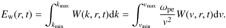 (10)To see the variation of Langmuir wave enhancement over thermal level as a function of distance, we normalised the level of Ew(r,t) by the local thermal level of Langmuir wave energy density, found from Eqs. (9) and (10) as
 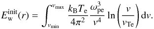 (11)To obtain a stopping frequency for type III bursts, we must quantify at what point in space (and hence what frequency) the electron beam stops generating high levels of Langmuir waves, required to emit type III radio bursts. We do this by calculating the maximum level of Langmuir wave energy density
  for every point of space and time. Again we normalise this by the thermal level of Langmuir wave energy density
  . By taking a fixed level for
  we are then able to estimate the lowest frequency an electron beam was able to induce this level of Langmuir wave energy density. We call this the stopping frequency.
3. Radial expansion of the guiding magnetic flux tubes
When electrons propagate outwards from the Sun, they follow the lines of decreasing magnetic field. As the magnetic flux tubes expand, so too does the electron beam, causing the beam density to decrease. An example cartoon showing this behaviour is given by Fig. 2 (left). We have modelled the expansion via the second term in Eq. (1). We use M(r) to model the cross-section of the expanding flux tube that the electrons are travelling along as a function of r and it takes the form  (12)where r0 is the characteristic length of the expansion of the magnetic flux tube. The power-law index β defines an expanding flux tube and the radial dependency of the magnetic field B ∝ M(r)-1 ∝ r− β. M0 = π(d/ 2)2 cm2 ≃ 80 Mm2 is the cross-sectional area of the flux tube at the centre of the acceleration site, r = 0. For r0 = 3.4 × 109 cm, an expansion of r2 gives a cone of angle 33 degrees, an angle that has been deduced from some in situ observations of high energy electrons near the Earth (e.g. Lin 1974; Steinberg et al. 1985; Krucker et al. 2007; Wang et al. 2012).
We have not changed the background density profile when changing the expansion of the magnetic flux tube. Whislt the magnetic field, solar wind speed and background electron density are all interdependent properties (e.g. solving Eqs. (12)−(14) in Kontar 2001a), it is beyond the scope of the paper to simulate how all three change with radial distance together. We focus on the effects of the magnetic field.
As the electron cloud propagates outwards along the expanding magnetic flux tube (Fig. 2), the electron number density decreases with the rate dependent on the flux tube expansion rate. Whilst velocity dispersion also causes an increases in the derivative ∂f/∂v that grows with distance, the decrease in beam density from the electrons following the expanding magnetic flux tube is greater. These two processes are not the entire picture but it is clear that the expansion of the magnetic flux tube is expected to be a major factor that governs when subsequent type III radio emission stops.
3.1. Simulations
To illustrate how the expansion of the magnetic flux tube can influence the propagation of an electron beam we numerically solved Eqs. (1), (2) with the parameters given in Sect. 2 except that we change the rate of magnetic flux expansion. For this we varied β in Eq. (12) such that β = 2, 2.5, 3, 3.5.
As described in Sect. 2.3 we used the Langmuir wave energy density as a proxy for the type III radio emission. We plot the Langmuir wave energy density variation as a function of time and frequency (see e.g. Fig. 3), similar to what is normally produced for type III bursts using the flux density of radio waves as a function of time and frequency. To account for the decreasing Langmuir wave energy as a function of frequency, shown in Eq. (10), we normalised the energy density by the thermal level of Langmuir waves given by  .
.
Figure 3 shows how the energy density of Langmuir waves varies as a function of frequency and time for all four values of β = 2, 2.5, 3, 3.5. When β = 3.5 (top left graph) the energy density in Langmuir waves is low, ceasing completely after only 0.8 mins and not reaching frequencies less than roughly 4 MHz. The magnetic flux tube expands very rapidly, causing the electron beam to decrease in density over a short distance and is consequently no longer able to drive the wave-particle interaction. When β = 3.0 (top right graph) the magnetic flux tube expands less rapidly and Langmuir waves are induced by the electron beam over a longer time (2.5 min) and at lower frequencies (1 MHz). This trend continues for β = 2.5 (bottom left graph) and β = 2.0 (bottom right graph) with the Langmuir wave energy density being significant over the thermal level at 0.1 MHz and 0.03 MHz respectively.
For different levels of magnetic flux tube expansion, Fig. 4 (left) shows the minimum background plasma frequency the electron beam was able to excite a certain level of Langmuir wave energy, as described in Sect. 2.2.1. We note that the background plasma frequency relates to distance using the density model described in Sect. 2.2.2. The different lines in Fig. 4 illustrate different values of , taken between 102 and 103.
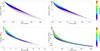 |
Fig. 3 Langmuir wave energy density |

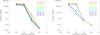 |
Fig. 4 Minimum frequency (stopping frequency) where an electron beam is able to induce certain amount of Langmuir wave energy density (see colour-coded lines). plotted against the different radial expansion exponents, β. The different coloured lines represent different levels of Langmuir wave energy (normalised by the thermal level) between 100 and 1000. The right graph includes density fluctuations in the background plasma. |
We can see from Fig. 4 that slow expansion (smaller β) leads to a significant energy of Langmuir waves at frequencies below ~1 MHz. The points representing different levels of maximum Langmuir wave energy density are closer together in minimum frequency for β = 2 compared to β = 2.5. As the electron beam propagates farther from the Sun, the plasma density profile becomes flatter, (| ∂ωpe/∂r | decreases) and hence the Langmuir wave energy decreases faster with frequency. The similarity between the simulations with β = 3.5 and β = 3.0 is because the electron beam density decreases very quickly in both simulations. In comparison to the cases β = 2, 2.5, only a small amount of energy is transferred to Langmuir waves before the wave generation is quenched.
When we consider weaker radial expansion (for instance β = 2), we observe Langmuir waves being generated at distances much farther from the Sun and consequently at much lower frequencies. We considered radial expansion with smaller β values of β = 1.5, 1.0 but they produced so much Langmuir wave energy that by 2 AU (the end of our simulation box) there was still a significant level of energy density in Langmuir waves, with  . As shown in the next section, part of this result is related to not considering the density fluctuations in the background plasma. These results support the idea (Buttighoffer et al. 1995; Buttighoffer 1998) that narrow flux tubes are encountered when electrons producing type III emission are observed with Ulysses at distances greater than 1 AU.
3.2. Complex radial expansion
In Eq. (12) the magnetic flux tube expands in the corona at the same rate as it expands in the heliosphere. Whilst this might be more relevant in areas of open field (for instance the coronal holes), solar active regions can be far from simplistic. It is possible that the magnetic field can be focussed in the corona through narrow flux tubes. From Sect. 3 we know this will facilitate a higher level of Langmuir wave turbulence. However, it has been observed that type III bursts can occur at high frequencies and not at lower frequencies. One explanation for this behaviour is an increased expansion as electrons propagate out of the corona. Figure 2 (right) shows a cartoon of the geometry of the magnetic field in such a scenario, where the expansion of the magnetic field lines increase at a certain height rc.
We model the magnetic field proposed in Fig. 2 (right) by modifying magnetic flux tube cross-sectional area M(r), so that![Mathematical equation: \begin{equation} \label{eqn:double_expansion} M(r) = M_0 \begin{cases} \left( 1 + \frac{r}{r_0}\right)^{\beta} & \mbox{for } r<r_{\rm c} \\ \left[\left(1 + \frac{r}{r_0}\right)^{\beta} + Z_{\rm c} \left( 1 - \frac{r}{r_{\rm c}}\right)^{\beta}\right] & \mbox{for } r\geq r_{\rm c}. \end{cases} \end{equation}](/articles/aa/full_html/2015/05/aa25309-14/aa25309-14-eq93.png) (13)where rc is a height above the photosphere where the expansion of the magnetic flux tube changes. Above this height the expansion is more rapid, with the severity of this increased expansion modelled through the constant Zc. Similar to Eq. (12), the constant M0 = 80 Mm is the cross-sectional area of the flux tube at the centre of the acceleration site r = 0.
(13)where rc is a height above the photosphere where the expansion of the magnetic flux tube changes. Above this height the expansion is more rapid, with the severity of this increased expansion modelled through the constant Zc. Similar to Eq. (12), the constant M0 = 80 Mm is the cross-sectional area of the flux tube at the centre of the acceleration site r = 0.
In Fig. 5, we set β = 3 for the magnetic flux tube expansion, so that magnetic field decreases as r-3. To simulate a reduced expansion in the corona we increased the value of r0 = 1010 cm. We set rc = 2 × 1010 cm and rc = 4 × 1010 cm to demonstrate expansion at two different heights above the photosphere that correspond roughly to 100 MHz and 50 MHz. For each height we have varied the constant Zc = 101,103,105 to show different rates of expansion.
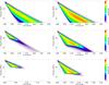 |
Fig. 5 Langmuir wave energy density |
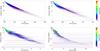 |
Fig. 6 Langmuir wave energy density |
Figure 5 shows the Langmuir wave energy density for the six different cases described above. Langmuir wave energy density is clearly reduced after the electron beam reaches rc when the expansion is significant. The two different frequencies of 100 MHz corresponding to rc = 2 × 1010 cm and 40 MHz corresponding to rc = 4 × 1010 cm are evident in Fig. 5 when Zc = 105, whereas Langmuir waves continue to be induced after the electron beam reaches rc when Zc = 10 (Fig. 5).
4. Density fluctuations in the background plasma
The expansion of the guiding magnetic flux tubes is not the only factor that determines the stopping distance of a type III burst. Density fluctuations in the background plasma are known to decrease the level of Langmuir waves induced by an electron beam (e.g. Ryutov 1969; Smith & Sime 1979; Melrose 1980a; Kontar 2001a; Reid & Kontar 2010, 2013; Li et al. 2012; Ratcliffe et al. 2012). Langmuir waves are shifted out of resonance with the electron beam by the density fluctuations that results in a decreased level of Langmuir wave turbulence.
The power spectrum of density fluctuations near the Earth has been observed to obey a Kolmogorov-type power law with a spectral index of − 5 / 3 (e.g. Celnikier et al. 1983, 1987; Chen et al. 2013). Following Reid & Kontar (2010), the spectrum of density fluctuations was modelled with spectral index − 5 / 3 between the wavelengths of 107 and 1010 cm, so that the new perturbed density profile is given by the following equation ![Mathematical equation: \begin{equation} \label{fluc} n_{\rm e}(r) = n_0(r)\left[1 + C(r)\sum_{n=1}^N\lambda_n^{\mu/2}\sin(2\pi r/\lambda_n + \phi_n)\right], \end{equation}](/articles/aa/full_html/2015/05/aa25309-14/aa25309-14-eq111.png) (14)where N = 1000 is the number of perturbations, n0(r) is the initial unperturbed density (defined in Sect. 2.2.2), λn is the wavelength of nth fluctuation, μ = 5 / 3 is the power-law spectral index in the power spectrum, and φn is the random phase of the individual fluctuations. C(r) is the normalisation that defines the level of density fluctuations
(14)where N = 1000 is the number of perturbations, n0(r) is the initial unperturbed density (defined in Sect. 2.2.2), λn is the wavelength of nth fluctuation, μ = 5 / 3 is the power-law spectral index in the power spectrum, and φn is the random phase of the individual fluctuations. C(r) is the normalisation that defines the level of density fluctuations 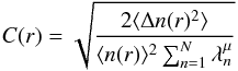 (15)where the rms deviation of the density
  is taken so that near the Earth at r = 1 AU
 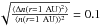 . Reid & Kontar (2010) used numerical simulations of electron beams travelling to the Earth to estimate C(r). The best fit was a level of fluctuations that decreased as a function of distance using the formula
 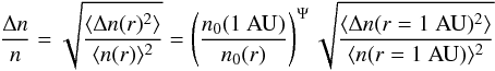 (16)where Ψ = 0.25. This results in a level of fluctuations (denoted now for simplicity as Δn/n) at the Sun that is roughly 1% of the level at the Earth, or Δn/n = 10-3. The value increases as a function of distance to Δn/n = 10-1 at the Earth.
4.1. Simulations
Using the same beam and plasma parameters as Sect. 3 we conducted the simulations with the inclusion of a fluctuating background plasma. We varied the expansion of the magnetic flux tubes using β = 2, 2.5, 3.0, 3.5. The normalised spectral energy density of Langmuir waves are presented as a function of time and plasma frequency in Fig. 6. The bursty nature of the Langmuir wave energy density is evident, especially comparing Figs. 6 to 3. The bursty nature of the Langmuir energy density in Fig. 6 is increased for lower frequencies because of the model that we used for density fluctuations. Equation (16) has a high intensity of density fluctuations farther away from the Sun.
Figure 4 (right) shows how the different levels of magnetic field expansion affects the minimum frequency of the background plasma that certain levels of Langmuir wave energy density are induced. A comparison with the case without fluctuations reveals that in general the inclusion of density fluctuations increases this minimum frequency. For instance at β = 2.0 an increased Langmuir wave energy density was not observed below 0.08 MHz compared to the 0.02 MHz with density fluctuations were not included. Density fluctuations in the background plasma are therefore another important parameter in the background plasma that affects the stopping frequency of type III bursts. Increasing the rms deviation of the density Δn/n given in Eq. (16) increases the suppression of Langmuir waves induced by the electron beam density, and vice versa.
We also point out that for any single value of β, the points in Fig. 4 are more closely spaced when density fluctuations are present in the background plasma. Indeed, all points are almost on top of each other when β = 2.0 or β = 2.5. These points are due to the spikes in the spatial distribution of Langmuir wave energy that reached at least 103 times that of the background level. The spikes are able to produce higher Langmuir wave energy density at lower background frequencies. For example a level around 103 is only observed at 5 MHz without fluctuations but at 0.5 MHz with fluctuations. However, the total Langmuir wave energy is lower when density fluctuations are considered.
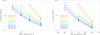 |
Fig. 7 Minimum frequency (stopping frequency) where an electron beam is able to induce certain level of Langmuir wave energy density (see colour-coded lines). Left: plotted against beam density. Right: plotted against velocity spectral index. The different coloured lines represent different levels of Langmuir wave energy (normalised by the thermal level) between 102 and 103. |
5. Role of initial electron beam parameters
In this section we explore how the different initial electron beam parameters can affect the stopping frequency of type III bursts. Specifically we look at the number of injected electrons and how they are distributed in energy space.
5.1. Injected beam density
Clearly the number of electrons we inject into the simulations is important when determining the level of Langmuir waves that is induced and consequently at what frequency the beam stops wave generation. As described in Sect. 5, the simulation parameter that dictates the number density of electrons injected into the simulation is nbeam3. Our simulations are set up as described in Sect. 2 with the guiding flux tube characterised using β = 2.5. We have varied the beam density over one order of magnitude such that nbeam = 5 × 106 cm-3, 2 × 106 cm-3, 1 × 106 cm-3,5 × 105 cm-3.
Similar to the previous sections, we have plotted the normalised maximum Langmuir wave energy density as a function of frequency in Fig. 7. As expected, the beams with higher initial densities are able to excite higher levels of Langmuir wave energy at lower plasma frequencies (or at distances farther away from the Sun). As the initial number of electrons in the beam is reduced, the beam is less and less able to generate Langmuir waves farther out. For beam density 5 × 105 cm-3 the beam is not able to excite  other than when it initially became unstable at frequencies >100 MHz, similar to the beams that experience high magnetic flux tube expansion in Fig. 5.
5.2. Injected beam energy distribution
The distribution of beam electrons as a function of energy is very important for the production of Langmuir waves. Exactly what distribution we inject into the simulation will have a very significant effect on the minimum frequency the beam can interact with Langmuir waves. The energy distribution is governed by the spectral index δ defined in Eq. (4). We demonstrate the importance by using simulations with the same parameters as Sect. 3, keeping the magnetic field expansion static using β = 2.5, and varying the velocity spectral index δ = 6,7,8.
We plot the normalised maximum Langmuir wave energy density  for these three initial spectral indices as a function of frequency in Fig. 7. We can see the frequencies corresponding to a high peak level of Langmuir wave energy density dramatically decreases as we decrease the initial velocity spectral index. As we have normalised the number density of electrons injected, if we lower the spectral index, more high energies are injected. There are two reasons this leads to higher level of Langmuir wave turbulence:
-
The injection altitude is relatively low in the corona (fpe = 500 MHz). The background density is 2 × 109 cm-3 where the collision rate is not negligible. Therefore the low energy electrons (e.g. ≲6 keV) collisionally lose energy before the beam escapes to a lower density background plasma. As demonstrated in Reid & Kontar (2013) the electrons with energy 1.5−6 keV will lose 99% of their energy after only 0.1 R⊙ of travel. A lower spectral index (harder spectrum) means that the beam loses less energy in the low corona and retains more energy to transfer to Langmuir waves.
-
Since the growth rate of Langmuir waves at one point in space is proportional to v2∂f/∂v, the v2 term means that a flatter initial electron spectrum will increase it.
6. Discussion and conclusions
To analyse the stopping frequency of type III radio bursts the outward propagation of deka-keV electrons have been modelled from a flaring acceleration site through the solar corona and inner heliosphere. The wave-particle interaction between electrons and Langmuir waves, Coulomb collisions, Langmuir wave refraction, and the radial expansion of the guiding magnetic flux tubes have been included. We have investigated the lowest frequency that the beam causes enhanced levels of Langmuir waves, and hence radio waves, for different electron beam and background plasma properties.
The radial expansion of the guiding magnetic flux tube significantly affects the distances from the Sun that electrons can induce high levels of Langmuir wave turbulence (and hence characteristic type III burst frequencies). The electron beam follows the expanding magnetic flux tube and consequently decreases in density as a function of distance from the Sun. The decrease in density eventually quenches the instability that causes Langmuir wave generation. This scenario could be the cause of type III bursts that are observed only at high frequencies although it is not the only mechanism that can produce such type III bursts.
Background density fluctuations caused an electron beam to cease producing Langmuir waves at shorter distances from the Sun. However, their effect on stopping frequencies was not as significant as varying the rate of magnetic flux tube expansion. Due to the clumping of Langmuir waves in space, caused by the density fluctuations, we were able to observe high level of Langmuir waves at reasonably low frequencies but the overall level of Langmuir waves was reduced.
Varying the properties of the injected electron beam also affects the lowest frequency where Langmuir waves production is significant. Decreasing the density of the injected electron beam or increasing the spectral index of the injected electron beam reduces the distance the electron beam can travel before it stops producing high levels of Langmuir wave turbulence. We then expect that less dense electron beams or beams with high spectral indices will have higher type III stopping frequencies. It is possible that injection of electrons at high altitudes ≳0.1 R⊙ would be less sensitive to the spectral index of the beam in respect to the type III stopping frequency due to a reduced role of Coulomb collisions.
How do these finding relate to some of the hypothesised reasons in Leblanc et al. (1995)? We find that all the different effects that govern the number of high energy electrons play some roles in the type III stopping frequency: the expansion of the guiding magnetic flux tubes, the injected beam density and the injected spectral index. We also found that large scale density fluctuations in the background electron density play a role, although a high level of density fluctuations may still cause irregular radio emission caused by the localised clumping of Langmuir waves. The hypothesis that we have not checked is how the other non-linear plasma processes required to convert Langmuir waves into radio waves affect the stopping frequency of type III bursts. What we have also explained is the prevalence for stronger type III bursts to have lower stopping frequencies, a result observed by Leblanc et al. (1995, 1996), Dulk et al. (1996). The beams with more deca-keV electrons produce in general higher levels of Langmuir waves, and consequently make brighter type IIIs and have lower stopping frequencies. The upcoming missions Solar Orbiter and Solar Probe Plus should help to observationally study the radial plasma properties with in situ measurements.
Magnetic flux tubes have been observed to expand super-radially (rates faster than r2) in the corona with type III radio emission following the magnetic flux tube expansion (e.g. Klein et al. 2008). Whilst this expansion can be large, it is very difficult to have a large expansion such that B ∝ r-3.5 and produce type III radio emission. The electron beam decreases in density too fast. To demonstrate this we injected an electron beam with the same characteristics described in Sect. 2.2.1 but with a spectral index of 5 in velocity space. Such a low spectral index is on the verge of what is inferred observationally from hard X-rays (see e.g. Kašparová et al. 2005). Figure 8 shows how the energy density of Langmuir waves varies as a function of time and frequency. We only observe a high level of Langmuir wave energy at the high frequencies and not at the low frequencies. A flare with such a low spectral index would almost certainly produce type III radio emission below 0.1 MHz, similar to Fig. 1. We conclude that we would not observe type III bursts if the solar magnetic field ever expands at such a super-radial rate.
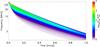 |
Fig. 8 Langmuir wave energy density Ew/Einit in plasma frequency – time plane. The coefficient that models the magnetic flux tube expansion is β = 3.5 and the velocity spectral index of injected electrons is α = 5. |
From type III burst simulations (Ratcliffe et al. 2014), it is evident that the spectrum of Langmuir wave energy density does not exactly reflect the spectrum of radio waves that are observed. The requirement for backscattered Langmuir waves to interact with forward propagating Langmuir waves in the production of harmonic emission means that spectral characteristics of Langmuir waves are important, not just the absolute energy density. However, the radial expansion of the magnetic flux tube reduces the Langmuir wave production. Therefore our conclusions on stopping frequency are expected to be mirrored in escaping radio emission, although a detailed study including the generation of radio emission can explore additional effects of wave-wave plasma processes on the type III stopping frequencies.
Since Langmuir waves do not propagate far before being re-absorbed, M(r) is not taken into account in Eq. (2).
Tsw used in the density model is different from the electron temperature Te that defines vTe.
nbeam is the time integrated beam density injected at the centre of the acceleration region. However, given the fast injection characteristic time of 10-3 s, we refer to it simply as the beam density.
Acknowledgments
We acknowledge support from the STFC consolidated grant ST/L000741/1. Hamish Reid acknowledges funding from a SUPA Advanced Fellowship. Support from a Marie Curie International Research Staff Exchange Scheme Radiosun PEOPLE-2011-IRSES-295272 RadioSun project is greatly appreciated. This work benefited from the Royal Society grant RG130642.
References
- Benz, A. O., Monstein, C., Beverland, M., Meyer, H., & Stuber, B. 2009, Sol. Phys., 260, 375 [NASA ADS] [CrossRef] [Google Scholar]
- Bian, N. H., Kontar, E. P., & Ratcliffe, H. 2014, J. Geophys. Res. (Space Phys.), 119, 4239 [NASA ADS] [CrossRef] [Google Scholar]
- Bougeret, J., Kaiser, M. L., Kellogg, P. J., et al. 1995, Space Sci. Rev., 71, 231 [NASA ADS] [CrossRef] [Google Scholar]
- Bougeret, J. L., Goetz, K., Kaiser, M. L., et al. 2008, Space Sci. Rev., 136, 487 [NASA ADS] [CrossRef] [Google Scholar]
- Buttighoffer, A. 1998, A&A, 335, 295 [NASA ADS] [Google Scholar]
- Buttighoffer, A., Pick, M., Roelof, E. C., et al. 1995, J. Geophys. Res., 100, 3369 [NASA ADS] [CrossRef] [Google Scholar]
- Celnikier, L. M., Harvey, C. C., Jegou, R., Moricet, P., & Kemp, M. 1983, A&A, 126, 293 [NASA ADS] [Google Scholar]
- Celnikier, L. M., Muschietti, L., & Goldman, M. V. 1987, A&A, 181, 138 [NASA ADS] [Google Scholar]
- Chen, C. H. K., Howes, G. G., Bonnell, J. W., et al. 2013, in AIP Conf. Ser. 1539, eds. G. P. Zank, J. Borovsky, R. Bruno, et al., 143 [Google Scholar]
- de Genouillac, G. V., & Escande, D. F. 1981, A&A, 94, 219 [NASA ADS] [Google Scholar]
- Dennis, B. R. 1988, Sol. Phys., 118, 49 [NASA ADS] [CrossRef] [Google Scholar]
- Drummond, W. E., & Pines, D. 1962, Nucl. Fusion Supp., 3, 1049 [Google Scholar]
- Dulk, G. A. 1985, ARA&A, 23, 169 [NASA ADS] [CrossRef] [Google Scholar]
- Dulk, G. A., Leblanc, Y., Bougeret, J.-L., & Hoang, S. 1996, Geophys. Res. Lett., 23, 1203 [NASA ADS] [CrossRef] [Google Scholar]
- Ginzburg, V. L., & Zhelezniakov, V. V. 1958, Sov. Astron., 2, 653 [Google Scholar]
- Goldman, M. V. 1983, Sol. Phys., 89, 403 [NASA ADS] [CrossRef] [Google Scholar]
- Grognard, R. J.-M. 1985, in Solar Radiophysics: Studies of Emission from the Sun at Metre Wavelengths (CUP), 253 [Google Scholar]
- Hannah, I. G., Kontar, E. P., & Sirenko, O. K. 2009, ApJ, 707, L45 [NASA ADS] [CrossRef] [Google Scholar]
- Hannah, I. G., Kontar, E. P., & Reid, H. A. S. 2013, A&A, 550, A51 [NASA ADS] [CrossRef] [EDP Sciences] [Google Scholar]
- Holman, G. D., Aschwanden, M. J., Aurass, H., et al. 2011, Space Sci. Rev., 159, 107 [NASA ADS] [CrossRef] [Google Scholar]
- Kašparová, J., Karlický, M., Kontar, E. P., Schwartz, R. A., & Dennis, B. R. 2005, Sol. Phys., 232, 63 [NASA ADS] [CrossRef] [Google Scholar]
- Klein, K.-L., Krucker, S., Lointier, G., & Kerdraon, A. 2008, A&A, 486, 589 [NASA ADS] [CrossRef] [EDP Sciences] [Google Scholar]
- Kontar, E. P. 2001a, Sol. Phys., 202, 131 [NASA ADS] [CrossRef] [Google Scholar]
- Kontar, E. P. 2001b, A&A, 375, 629 [NASA ADS] [CrossRef] [EDP Sciences] [Google Scholar]
- Kontar, E. P. 2001c, Comp. Phys. Comm., 138, 222 [Google Scholar]
- Kontar, E. P., & Reid, H. A. S. 2009, ApJ, 695, L140 [NASA ADS] [CrossRef] [Google Scholar]
- Kontar, E. P., Lapshin, V. I., & Mel’Nik, V. N. 1998, Plasm. Phys. Rep., 24, 772 [Google Scholar]
- Krucker, S., Kontar, E. P., Christe, S., & Lin, R. P. 2007, ApJ, 663, L109 [Google Scholar]
- Krupar, V., Maksimovic, M., Santolik, O., et al. 2014, Sol. Phys., 289, 3121 [NASA ADS] [CrossRef] [Google Scholar]
- Leblanc, Y., Dulk, G. A., & Hoang, S. 1995, Geophys. Res. Lett., 22, 3429 [NASA ADS] [CrossRef] [Google Scholar]
- Leblanc, Y., Dulk, G. A., Hoang, S., Bougeret, J.-L., & Robinson, P. A. 1996, A&A, 316, 406 [NASA ADS] [Google Scholar]
- Lecacheux, A. 2000, Geophysical Monograph Series (Washington, DC: AGU), 119, 321 [Google Scholar]
- Ledenev, V. G., Zverev, E. A., & Starygin, A. P. 2004, Sol. Phys., 222, 299 [NASA ADS] [CrossRef] [Google Scholar]
- Li, B., & Cairns, I. H. 2014, Sol. Phys., 289, 951 [NASA ADS] [CrossRef] [Google Scholar]
- Li, B., Cairns, I. H., & Robinson, P. A. 2008, J. Geophys. Res. (Space Phys.), 113, 6104 [NASA ADS] [CrossRef] [Google Scholar]
- Li, B., Cairns, I. H., Yan, Y. H., & Robinson, P. A. 2011, ApJ, 738, L9 [NASA ADS] [CrossRef] [Google Scholar]
- Li, B., Cairns, I. H., & Robinson, P. A. 2012, Sol. Phys., 279, 173 [NASA ADS] [CrossRef] [Google Scholar]
- Lin, R. P. 1974, Space Sci. Rev., 16, 189 [NASA ADS] [CrossRef] [Google Scholar]
- Magelssen, G. R., & Smith, D. F. 1977, Sol. Phys., 55, 211 [NASA ADS] [CrossRef] [Google Scholar]
- Maksimovic, M., Zouganelis, I., Chaufray, J., et al. 2005, J. Geophys. Res. (Space Phys.), 110, 9104 [NASA ADS] [CrossRef] [Google Scholar]
- Mann, G., Jansen, F., MacDowall, R. J., Kaiser, M. L., & Stone, R. G. 1999, A&A, 348, 614 [NASA ADS] [Google Scholar]
- Mel’Nik, V. N. 1995, Plasma Phys. Rep., 21, 89 [Google Scholar]
- Mel’Nik, V. N. 2003, Sol. Phys., 212, 111 [NASA ADS] [CrossRef] [Google Scholar]
- Melrose, D. B. 1980a, Plasma astrohysics. Nonthermal processes in diffuse magnetized plasmas, Vol. 1, The emission, absorption and transfer of waves in plasmas, Vol. 2, Astrophysical applications (New York: Gordon and Breach) [Google Scholar]
- Melrose, D. B. 1980b, Space Sci. Rev., 26, 3 [NASA ADS] [CrossRef] [Google Scholar]
- Melrose, D. B. 1987, Sol. Phys., 111, 89 [NASA ADS] [CrossRef] [Google Scholar]
- Melrose, D. B. 1990, Sol. Phys., 130, 3 [NASA ADS] [CrossRef] [Google Scholar]
- Muschietti, L. 1990, Sol. Phys., 130, 201 [NASA ADS] [CrossRef] [Google Scholar]
- Muschietti, L., Goldman, M. V., & Newman, D. 1985, Sol. Phys., 96, 181 [NASA ADS] [CrossRef] [Google Scholar]
- Nishikawa, K., & Ryutov, D. D. 1976, J. Phys. Soc. Japan, 41, 1757 [NASA ADS] [CrossRef] [Google Scholar]
- Parker, E. N. 1958, ApJ, 128, 664 [Google Scholar]
- Ratcliffe, H., & Kontar, E. P. 2014, A&A, 562, A57 [NASA ADS] [CrossRef] [EDP Sciences] [Google Scholar]
- Ratcliffe, H., Bian, N. H., & Kontar, E. P. 2012, ApJ, 761, 176 [NASA ADS] [CrossRef] [Google Scholar]
- Ratcliffe, H., Kontar, E. P., & Reid, H. A. S. 2014, A&A, 572, A111 [NASA ADS] [CrossRef] [EDP Sciences] [Google Scholar]
- Reid, H. A. S., & Kontar, E. P. 2010, ApJ, 721, 864 [NASA ADS] [CrossRef] [Google Scholar]
- Reid, H. A. S., & Kontar, E. P. 2013, Sol. Phys., 285, 217 [NASA ADS] [CrossRef] [Google Scholar]
- Reid, H. A. S., & Ratcliffe, H. 2014, RA&A, 14, 773 [Google Scholar]
- Reid, H. A. S., Vilmer, N., & Kontar, E. P. 2011, A&A, 529, A66 [NASA ADS] [CrossRef] [EDP Sciences] [Google Scholar]
- Reid, H. A. S., Vilmer, N., & Kontar, E. P. 2014, A&A, 567, A85 [NASA ADS] [CrossRef] [EDP Sciences] [Google Scholar]
- Robinson, P. A. 1992, Sol. Phys., 137, 307 [NASA ADS] [CrossRef] [Google Scholar]
- Ryutov, D. D. 1969, Sov. J. Exper. Theor. Phys., 30, 131 [Google Scholar]
- Smith, D. F. 1970, Sol. Phys., 15, 202 [NASA ADS] [CrossRef] [Google Scholar]
- Smith, D. F., & Sime, D. 1979, ApJ, 233, 998 [NASA ADS] [CrossRef] [Google Scholar]
- Smith, R. A., Goldstein, M. L., & Papadopoulos, K. 1976, Sol. Phys., 46, 515 [NASA ADS] [CrossRef] [Google Scholar]
- Steinberg, J. L., Hoang, S., & Dulk, G. A. 1985, A&A, 150, 205 [NASA ADS] [Google Scholar]
- Stone, R. G., Pedersen, B. M., Harvey, C. C., et al. 1992, Science, 257, 1524 [NASA ADS] [CrossRef] [Google Scholar]
- Suzuki, S., & Dulk, G. A. 1985, Bursts of Type III and Type V (Solar Radiophysics: Studies of Emission from the Sun at Metre Wavelengths), 289 [Google Scholar]
- Takakura, T., & Shibahashi, H. 1976, Sol. Phys., 46, 323 [NASA ADS] [CrossRef] [Google Scholar]
- Tsiklauri, D. 2010, Sol. Phys., 267, 393 [NASA ADS] [CrossRef] [Google Scholar]
- Tsiklauri, D. 2011, Phys. Plasmas, 18, 052903 [NASA ADS] [CrossRef] [Google Scholar]
- Vedenov, A. A., Lelikhov, E. P., & Sagdeev, R. Z. 1962, Nucl. Fusion Supp., 2, 465 [Google Scholar]
- Wang, L., Lin, R. P., Krucker, S., & Mason, G. M. 2012, ApJ, 759, 69 [NASA ADS] [CrossRef] [Google Scholar]
- Wild, J. P., & McCready, L. L. 1950, Austr. J. Sci. Res. A Phys. Sci., 3, 387 [Google Scholar]
- Zaitsev, V. V., Mityakov, N. A., & Rapoport, V. O. 1972, Sol. Phys., 24, 444 [NASA ADS] [CrossRef] [Google Scholar]
- Zheleznyakov, V. V., & Zaitsev, V. V. 1970, Sov. Astron., 14, 47 [NASA ADS] [Google Scholar]
All Figures
|
Fig. 1 Example of many type III bursts on 16 February 2014, detected by the WAVES instrument on the WIND spacecraft at 14−0.02 MHz (Bougeret et al. 1995), the Nançay Decametre Array at 80−14 MHz (Lecacheux 2000) and Phoenix 4 at 900−200 MHz (Benz et al. 2009). The large type III burst at 09:30 was associated with a GOES M1 flare. We can observe type III bursts stopping at a variety of different frequencies. The periodicity observed below 1 MHz is an artefact. |
| In the text | |
|
Fig. 2 Cartoon of an electron cloud (green) travelling upwards from an acceleration region through the corona, following the magnetic field. The density of the electron cloud is represented through the transparency. Left: an example of a constant radial expansion described by Eq. (12). Right: at a critical height rc the magnetic field lines begin to expand at an increased rate described by Eq. (13), causing the density of the electron cloud to decrease faster. |
| In the text | |
|
Fig. 3 Langmuir wave energy density |
| In the text | |
|
Fig. 4 Minimum frequency (stopping frequency) where an electron beam is able to induce certain amount of Langmuir wave energy density (see colour-coded lines). plotted against the different radial expansion exponents, β. The different coloured lines represent different levels of Langmuir wave energy (normalised by the thermal level) between 100 and 1000. The right graph includes density fluctuations in the background plasma. |
| In the text | |
|
Fig. 5 Langmuir wave energy density |
| In the text | |
|
Fig. 6 Langmuir wave energy density |
| In the text | |
|
Fig. 7 Minimum frequency (stopping frequency) where an electron beam is able to induce certain level of Langmuir wave energy density (see colour-coded lines). Left: plotted against beam density. Right: plotted against velocity spectral index. The different coloured lines represent different levels of Langmuir wave energy (normalised by the thermal level) between 102 and 103. |
| In the text | |
|
Fig. 8 Langmuir wave energy density Ew/Einit in plasma frequency – time plane. The coefficient that models the magnetic flux tube expansion is β = 3.5 and the velocity spectral index of injected electrons is α = 5. |
| In the text | |
Current usage metrics show cumulative count of Article Views (full-text article views including HTML views, PDF and ePub downloads, according to the available data) and Abstracts Views on Vision4Press platform.
Data correspond to usage on the plateform after 2015. The current usage metrics is available 48-96 hours after online publication and is updated daily on week days.
Initial download of the metrics may take a while.