| Issue |
A&A
Volume 577, May 2015
|
|
|---|---|---|
| Article Number | A92 | |
| Number of page(s) | 10 | |
| Section | The Sun | |
| DOI | https://doi.org/10.1051/0004-6361/201425138 | |
| Published online | 08 May 2015 | |
Non-LTE modelling of prominence fine structures using hydrogen Lyman-line profiles
1
Astronomical Institute of Slovak Academy of Sciences,
05960
Tatranská Lomnica,
Slovak Republic
e-mail:
pschwartz@astro.sk
2
School of Mathematics and Statistics, University of St.
Andrews, North Haugh, St.
Andrews, Fife,
KY16 9SS,
UK
3
Max-Planck-Institut für Sonnensystemforschung,
Justus-von-Liebig-Weg 3,
37077
Göttingen,
Germany
4
Astronomical Institute, Academy of Sciences of the Czech
Republic, 25165
Ondřejov, Czech
Republic
Received: 10 October 2014
Accepted: 10 March 2015
Aims. We perform a detailed statistical analysis of the spectral Lyman-line observations of the quiescent prominence observed on May 18, 2005.
Methods. We used a profile-to-profile comparison of the synthetic Lyman spectra obtained by 2D single-thread prominence fine-structure model as a starting point for a full statistical analysis of the observed Lyman spectra. We employed 2D multi-thread fine-structure models with random positions and line-of-sight velocities of each thread to obtain a statistically significant set of synthetic Lyman-line profiles. We used for the first time multi-thread models composed of non-identical threads and viewed at line-of-sight angles different from perpendicular to the magnetic field.
Results. We investigated the plasma properties of the prominence observed with the SoHO/SUMER spectrograph on May 18, 2005 by comparing the histograms of three statistical parameters characterizing the properties of the synthetic and observed line profiles. In this way, the integrated intensity, Lyman decrement ratio, and the ratio of intensity at the central reversal to the average intensity of peaks provided insight into the column mass and the central temperature of the prominence fine structures.
Key words: Sun: filaments, prominences / line: profiles / radiative transfer / methods: statistical
© ESO, 2015
1. Introduction
Spectral observations of the quiescent solar prominences in hydrogen Lyman lines and continuum represent a unique tool for probing of their structure and physical properties. A substantial amount of prominence spectral data in Lyman lines was provided by the Solar Ultraviolet Measurements of Emitted Radiation (SUMER) UV-spectrograph (Wilhelm et al. 1995) onboard the Solar and Heliospheric Observatory (SoHO) satellite. Prominence observations made with instruments onboard SoHO were reviewed by Patsourakos & Vial (2002); see also a review of the prominence fine structures by Heinzel (2007).
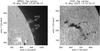 |
Fig. 1 Left panel: part of the full-disk Hα line-centre filtergram obtained by BBSO/NST on 18 May 2005. Vertical bar marks the position of the SoHO/SUMER slit. Spectra were obtained only from the part of the slit that is marked by the solid line because the SUMER detector was partially damaged. Right panel: prominence seen as a filament in part of the full-disk observations in the Hα line centre made at the Kanzelhöhe Solar Observatory three days earlier. The two clearly visible Hα features marked by arrows and denoted as NHS and SHS are the northern and southern Hα prominence structures. |
Interpreting the prominence observations in the Lyman lines requires sophisticated models of the prominence plasma in the magnetic field and complex non-LTE radiative transfer computations. Such models were first developed by Poland & Anzer (1971) and Heasley & Mihalas (1976). Later, Gouttebroze et al. (1993) used a sophisticated hydrogen atom with more than 20 levels plus continuum and a large grid of 1D isothermal isobaric slab models. This was followed by Anzer & Heinzel (1998, 1999), who developed 1D magnetohydrostatic equilibrium models of the Kippenhahn-Schlüter (K-S) type. These were generalized into 2D by Heinzel & Anzer (2001), whose prominence fine-structure models take the form of 2D vertically infinite plasma threads in magnetohydrostatic equilibrium, suspended in magnetic dips. The temperature structure of these prominence fine-structure threads is described semi-empirically and includes the prominence-corona transition region (PCTR). The substantial influence of the PCTR on the Lyman-line intensities was demonstrated by Anzer & Heinzel (1999). Two-dimensional vertically infinite prominence fine-structure models, but with the cylindrical cross-section, were also developed by Gouttebroze (2006).
The importance of the multi-thread prominence fine-structure models was shown by Gunár et al. (2007), who used a trial-and-error method to reproduce the observed Lyman spectrum. Later, Gunár et al. (2008) added random line-of-sight (LOS) macroscopic velocities to each thread of the multi-thread model, thus showing that even relatively low LOS velocities (of about 10 km s-1) have a significant effect on the asymmetries of the Lyman line profiles. Multi-thread models with randomly distributed LOS velocities of individual threads were shown by Gunár et al. (2010) to produce synthetic Lyman spectra that agree well with observations on the profile-to-profile as well as on statistical bases. Moreover, Berlicki et al. (2011) and Gunár et al. (2012) showed that the synthetic Hα spectra produced by multi-thread prominence fine-structure models also agree with the observations. Furthermore, Gunár et al. (2011a) and Gunár et al. (2011b) demonstrated that the temperature and electron density structures of these models lead to the synthetic differential emission-measure curves that agree well with the observations. Recently, Gunár et al. (2014) combined the multi-thread prominence fine-structure models with the 3D prominence magnetic field modelling to analyse a prominence observed on 22 June 2010.
Current reviews of the prominence physics can be found in Labrosse et al. (2010) and Mackay et al. (2010) and also in the review of the prominence fine-structure modelling by Gunár (2014).
In Sect. 2 we describe the observations in detail. Section 3 provides details of the prominence fine-structure modelling. In Sect. 4 we present our results, Sect. 5 contains the discussion, and Sect. 6 provides the conclusions.
2. Observations
A quiescent prominence was observed on the NW limb of the Sun by the SUMER spectrograph onboard the SoHO satellite. The observations were made during the fifteenth MEDOC observing campaign between 18 May 2005 22:01:12 and 19 May 2005 01:37:19 UT with static slit position (sit-and-stare observations). The position of the SoHO/SUMER spectrograph slit is shown in the left panel of Fig. 1 on the Hα line-centre filtergram from National Solar Telescope (NST; Goode et al.2003) at Big Bear Solar Observatory (BBSO). The co-alignment was achieved by correlating the distributions of BBSO/NST Hα data and the integrated Lyα SoHO/SUMER intensities along the slit. Usable SUMER data were obtained from only 40 pixels on the northern part of the SUMER slit because other part of detector A was damaged. The usable part of the slit, marked by the full line in Fig. 1, crosses a large column-like prominence structure oriented radially, which contains cool (T ≤ 10 000 K) plasma where the Hα line is formed. Another similar smaller structure is visible to the south. In Fig. 1 we mark these two features as the northern and southern Hα prominence structures. In the right panel of Fig. 1 the prominence is seen as a filament in the Hα filtergram made two days earlier by the Patrol Telescope for Solar Observations located at the Kanzelhöhe Solar Observatory. The two Hα prominence structures are clearly visible as two individual filamentary objects marked by arrows.
Properties of the SOHO/SUMER observations.
Complete hydrogen Lyman series were observed by SUMER in four spectral windows: 1215.6 Å, 1025.0 Å, 972.0 Å, and 940 Å, each with a wavelength range of approximately 45 Å and a cadence of 1–2 min. The basic properties of this set of observations are shown in Table 1. The observed spectra were reduced and calibrated using standard SolarSoft procedures. The spectral lines were identified using the SUMER spectral atlas of Curdt et al. (2001).
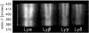 |
Fig. 2 Calibrated spectra of the Lyα–Lyδ lines. The spectra were corrected for vertical shifts. The vertical white bar marks the usable part of the slit. |
We note that the spectral image on the detector is inclined with respect to the direction of dispersion as a result of the different orientation of the grating and the detector. This causes two spectral lines with different wavelengths to be shifted with respect to each other. Moreover, displacement of the slit image on the detector due to non-linearity of the grating focus mechanism causes additional cross-dispersion shifts (Schühle 2003). Vertical shifts of the Lyβ and the higher Lyman lines with respect to the Lyα line were estimated by a comparison of the integrated intensity distributions and line profile shapes along the slit. Owing to the low signal-to-noise ratio in the spectra of the Ly5 and higher Lyman lines, only profiles of the Lyα–Lyδ lines were used in our analysis. An example of calibrated and corrected spectra of the four Lyman lines from one observation of the sit-and-stare observing sequence is shown in Fig. 2.
The Lyα line was placed on a so-called bare part of the detector A – outside the KBr coating and the attenuator. To protect the detector from further damage caused by high Lyα intensity, a lower detector voltage of 5390 V (standard is 5656 V) was set during the Lyα observations. As was shown by Schwartz et al. (2012), calibration is only marginally affected (by less than 2%) at such lower voltage. Other Lyman lines were observed with the standard voltage. A similar set of Lyman-line observations with lower voltage for the Lyα line was also used by Gunár et al. (2010).
3. Prominence fine-structure modelling
Quiescent solar prominences are not homogeneous, but are composed of numerous fine structures, often quasi-vertical threads (see e.g. the review by Heinzel 2007). To analyse the Lyman spectra observations of these structures, we used the 2D prominence fine structure model of Heinzel & Anzer (2001) in the multi-thread configuration including the random LOS velocities of individual threads developed by Gunár et al. (2008). In this section we briefly describe the single- and multi-thread models and show the results of the statistical comparison of the synthetic Lyman line profiles with observed data.
3.1. Single-thread model
The 2D prominence fine structure model of Heinzel & Anzer (2001) approximates prominence quasi-vertical threads by a vertically infinite 2D structure embedded in a horizontal dipped magnetic field. The plasma in the thread is in the local magneto-hydrostatic (MHS) equilibrium of Kippenhahn-Schlüter type. The thread is symmetrically irradiated at all four sides by diluted (height-dependent) radiation from the solar surface. The dimension across the magnetic field – y coordinate – is fixed, but the dimension along the field – x coordinate – is determined by the MHS equilibrium. The centre of the coordinate system is fixed in the centre of the thread. Instead of the geometrical x-scale, the column mass m-scale was used in the direction along the magnetic field. The total column mass M(y) along a magnetic field line at a position y is defined as (Heinzel & Anzer 2001) 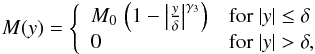 (1)where M0 is the column mass at the centre of the thread (at y = 0), δ is half of the dimension of the thread across the magnetic field, and γ3 is the exponent describing the column mass gradient across the magnetic field. We assumed here γ3 = 2. The 2D temperature structure of the thread in m − y scale is defined as (Heinzel & Anzer 2001)
![\begin{eqnarray} T(m,y) & = & T_{\mathrm{cen}}(y)+\left[T_{\mathrm{tr}}-T_{\mathrm{cen}}(y)\right]\left\{1-4\frac{m}{M(y)}\right. \nonumber \\[-1.5ex] & & \label{eq:tmy} \\[-1.5ex] & & \!\quad \quad\quad \quad \quad \quad\quad \quad \quad\quad\left.\times\left[\rule{0ex}{3ex}1-\frac{m}{M(y)}\right]\right\}^{\gamma_1}, \nonumber \end{eqnarray}](/articles/aa/full_html/2015/05/aa25138-14/aa25138-14-eq32.png) (2)where Ttr is the temperature at the thread boundary and γ1 is the exponent describing the temperature gradient along the magnetic field. Tcen(y) is the temperature at the dip centre at a position y and is defined as (Heinzel & Anzer 2001)
(2)where Ttr is the temperature at the thread boundary and γ1 is the exponent describing the temperature gradient along the magnetic field. Tcen(y) is the temperature at the dip centre at a position y and is defined as (Heinzel & Anzer 2001) 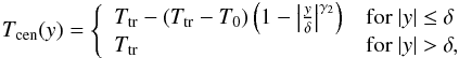 (3)where T0 is the minimum temperature at the thread centre (x = 0, y = 0) and γ2 is the exponent describing the temperature gradient across the magnetic field. This together with two additional input parameters of the model – the gas pressure p0 at the thread boundary and the horizontal component of the magnetic field Bx(0) in the dip centre – defines the distribution of the gas pressure p(x,y) in the thread.
 |
Fig. 3 Example of the temperature and gas-pressure distributions produced by the 2D single-thread model with the best agreement with observed spectra. The temperature step between contours is 10 000 K, that of the gas pressure is 0.02 dyn/cm2. |
Thus, the 2D vertical-thread model of the thread has 11 input parameters: the column mass M0, the dimension across the magnetic field Δy = 2δ, the temperatures at the boundary Ttr and at the centre T0, the central horizontal magnetic field Bx(0), the boundary gas pressure p0, the exponents γ1, γ2, γ3, the abundance of helium A(He) with respect to hydrogen (here we used 0.1), and the ratio of the microturbulence and sound velocities ε (we adopted ε = 0.5). We assumed the dimension of the threads in the direction across the magnetic field 2δ to be 1000 km. Temperatures in the PCTR reach up to the coronal values, but because hydrogen spectral lines are formed at temperatures well below 100 000 K, we adopted this value for Ttr. Examples of the temperature and gas-pressure distributions in the 2D thread are shown in Fig. 3.
We solved the 2D non-LTE radiative transfer by employing the Multilevel Accelerated Lambda Iterations (MALI; Auer & Paletou 1994) in the short characteristics method (Kunasz & Auer 1988). To solve the statistical equilibrium, we used a hydrogen atom with 12 levels plus continuum. Partial frequency redistribution (PRD) was assumed for the Lyα and Lyβ lines. For the higher Lyman lines the complete frequency redistribution was assumed.
3.2. Multi-thread model
As was shown by Gunár et al. (2007), the observed intensities in the peaks and near wings of the Lyβ and higher Lyman lines are better reproduced by multi-thread prominence fine-structure models than by models with only one thread. At the same time, the intensities in the centre of these lines produced by single-thread and multi-thread models are the same. This can be explained by the fact that in the line centre, where optical thickness is very large, only radiation from the foremost fine-structure thread can be seen. In contrast, the optical thickness in peaks is much lower and thus also the radiation from the threads farther away from the observer contributes to the measured intensities. This effect is more pronounced for the higher members of the Lyman line series, but is negligible for the Lyα line because of its large optical thickness even in the near wings. The multi-thread model used in this work (Gunár et al. 2008) was constructed in such a way that the foremost thread (the one closest to the observer) was fixed in the centre of the computational domain. The other threads were shifted to the left or right along the magnetic field with a maximum displacement equal to the half of the x-dimension of the thread. The distance between the threads was fixed to 1000 Km. The mutual irradiation of threads was not taken into account. As was shown by Gunár et al. (2008), assigning various LOS velocities to individual threads of such a multi-thread model can explain the observed asymmetries in the Lyman-line profiles.
The total intensity Iλ(total) along a given LOS emerging from the multi-thread model composed of N threads with random LOS velocities (see scheme in Fig. 4) was calculated using the following recurrent formula (derived from Eq. (1) of Gunár et al.2008) with j increasing from 2 to N:  (4)where
  and
and  . The intensity emerging from the jth thread of the multi-thread model is denoted as
  , Iλ(j ) is the intensity radiated by the jth thread itself, and τλ(j ) is its optical thickness. The latter two quantities are defined in the observer’s frame as
![\begin{eqnarray} I_{\lambda}\left(j\rule{0pt}{1.7ex}\,\right) & \equiv & I\left(\lambda-\Delta\lambda\left(j\rule{0pt}{1.7ex}\,\right) \rule{0pt}{2ex}\right) \label{eq:ilamdef} \\[-0.5ex] \tau\left(j\rule{0pt}{1.7ex}\,\right) & \equiv & \tau\left(\lambda-\Delta\lambda\left(j\rule{0pt}{1.7ex}\,\right) \rule{0pt}{2ex}\right) \label{eq:taulamdef}. \end{eqnarray}](/articles/aa/full_html/2015/05/aa25138-14/aa25138-14-eq58.png) The quantity Δλ(j ) is the Doppler shift for the jth thread corresponding to its LOS velocity ξ(j ):
The quantity Δλ(j ) is the Doppler shift for the jth thread corresponding to its LOS velocity ξ(j ):  (7)where λ0 is the central wavelength of a given spectral line and c the speed of light in vacuum. Positive values of ξ(j ) represent velocities oriented towards the observer. Here we used LOS velocities from the interval of ±10 km s-1. Equation (4) can be adapted to obtain the total emerging intensities also along the LOS not perpendicular to the magnetic field. In this case, parameter μ (the cosine of the angle between the actual LOS and the direction perpendicular to the magnetic field) is introduced.
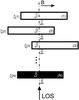 |
Fig. 4 Scheme of the prominence multi-thread model composed of N threads and LOS perpendicular to the magnetic field. Quantities ξ(j) represent the LOS velocities of individual threads. |
We obtained the distributions of the absorption and emission coefficient for individual threads with the 2D single-thread model described in the previous section. The Iλ(j ) intensities for the given value of μ were calculated by the quadrature form of Mihalas et al. (1978) for the formal solution of radiative transfer. More details can be found in Gunár et al. (2008).
3.3. Statistical comparison of observed and synthetic profiles
Previously, Gunár et al. (2010) used a 2D multi-thread model composed of identical threads for a statistical analysis of the promincence observed on May 25, 2005. Here we employed the multi-thread models with identical and, for the first time, also non-identical threads. For the non-identical threads we assumed higher values of the central minimum temperatures T0 in threads at the edges of the multi-thread model. Moreover, we used for the first time the LOS angles different from the perpendicular to the magnetic field in the statistical analysis. We do not aim to determine the exact configuration of the multi-thread model with randomly generated shifts and LOS velocities of individual threads. To perform the statistical analysis, we instead estimated the input parameters of the single-thread model by comparing the synthetic and observed Lyα profiles. The Lyα line is suitable for this because of its large optical thickness, which means that its profiles are contributed mainly from the foremost thread of any multi-thread setup. The multi-thread model is then constructed from individual threads with input parameters determined in this way. The same method was used by Gunár et al. (2010). When synthetic Lyman line profiles for a large number of realizations of the multi-thread model are calculated, the characteristics of the synthetic profiles can be statistically compared with large sets of observed profiles. Multiple observations of prominences with a static slit (sit-and-stare mode) are suitable for such a study. We used three statistical characteristics of the Lyman-line profiles: integrated intensity, Lyman decrement – ratio of the integrated intensity of a given line to the Lyβ integrated intensity, and depth of the reversal – ratio of intensity at the central reversal to average intensity of peaks (the so-called centre-to-peak ratio). The centre-to-peak ratio for both the synthetic and observed profiles was determined as follows (see also Gunár et al.2010): first, positions of the two peaks in a profile were found and the ratio was calculated by dividing the minimum intensity in wavelength interval between the peaks by the mean intensity of the peaks. To eliminate the influence of the noise on the estimation of the center-to-peak ratio, average intensities from three wavelength pixels at the reversal minimum and at each peak were used in the observed data. For profiles without reversal, the centre-to-peak ratios were not estimated, and these profiles were excluded from the statistical analysis of the reversal depth, but not from the analysis of the other two parameters. Gunár et al. (2010) used an additional characteristic quantifying the asymmetry of profiles with reversal. We did not use this here because it is sensitive mostly to the values of the LOS velocities, which are not the main interest of this study. The synthetic spectra obtained by the multi-thread model were resampled from the virtual slit scale (the actual x-y grid of the model seen with an angle μ) into the SUMER slit scale. One pixel along the SUMER slit is equivalent to one arcsec, which is equal to 726 km on the solar limb at the date of observations. The observed profiles of the Lyman lines are mainly blended by Balmer lines of He ii and by UV lines of O i. These blends need to be taken into account when deriving the three statistical characteristics. Approximate contributions of blends to the Lyman-line profiles were estimated by fitting the blending lines with Gaussian functions, using the data averaged along the slit.
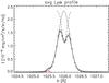 |
Fig. 5 Example of fitting of a Lyα profile to estimate the influence of a blend on the three profile characteristics. Observed data are plotted with stars, while the resulting fitted profile (including blends) is plotted as a thick full line. The Voigt function fitting the profile in the wings is plotted as a thin solid line and the negative Gaussian in the profile reversal as a dashed line. The blend occurring at approximately 1025.5 Å was fitted with the Gaussian and is plotted in red. |
The shape of the observed Lyman-line profiles were reproduced with the Voigt function in the wings and with a negative Gaussian in the central reversal, as is shown in an example of the Lyα profile in Fig. 5. This shows that even non-symmetrical profiles can be fitted by this method. The profiles were fitted with the Levemberg-Marquardt method. The negative Gaussian used for fitting the central reversals has no physical meaning, it was only used to reproduce the shape of the Lyman-line profiles without blends with the highest achievable accuracy. It is important to note that the fitting of the observed profiles was not used to derive the three profile characteristics. It was used only to estimate the influence of blends on the three profile characteristics estimated from the observed profiles. However, only blends located outside the Lyman-line cores that were sufficiently intense could be removed. For the Lyα line the influence of blends on all profile characteristics is negligible. We estimate the contributions of blends to the integrated intensities of higher Lyman lines to be 2.8% for Lyβ, 6.3% for Lyγ, and 7.8% for Lyδ. These contributions were subtracted from the integrated intensities of the observed profiles. Blends do not significantly influence the other two statistical characteristics used here.
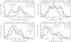 |
Fig. 6 Compared histograms of the integrated intensities of the observed and synthetic Lyα to Lyδ line profiles. The solid black line represents the observed data. Three values of μ are represented by corresponding colours and line-styles. |
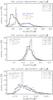 |
Fig. 7 Compared histograms of the Lyman decrement of observed and synthetic Lyman-line profiles. The solid black line represents the observed data. Three values of μ are represented by corresponding colours and line-styles. |
4. Results
4.1. Multi-thread model with identical threads
To obtain the best possible agreement between synthetic profiles obtained by the multi-thread model and the observations, we proceeded as follows. Several sets of single-thread models that each produced synthetic Lyα profiles similar to the observed ones were identified by trial and error. Then we selected from each such set the single-thread model with the least χ2 between the observed and synthetic Lyα profiles. Next, synthetic Lyα to Lyδ profiles were calculated for multiple configurations (random shifts and LOS velocities) of the multi-thread model with ten identical threads for each of the selected single-thread models. We calculated the synthetic profiles for various LOS angles μ. Three statistical characteristics of the synthetic profiles (see Sect. 3.3) were then compared with observations. Finally, a unique single-thread model with the best agreement of statistical characteristics of synthetic and observed profiles was identified. The input parameters of this model are the following:  The distributions of the temperature and gas pressure of this single-thread model are shown in Fig. 3.
The set of observed profiles contains 2160 Lyα profiles and 4320 profiles of each of the higher three Lyman lines. We compared the profile characteristics of such statistically significant set of observed data with the characteristics of 30 000 synthetic profiles of each of the four Lyman lines calculated with the multi-thread model. That means 300 profiles along the virtual SUMER slit corresponding to the size of the multi-thread structure in 100 realisations of the multi-thread model.
In Fig. 6 we show the histograms of the integrated intensity of the Lyα to Lyδ synthetic profiles obtained with the multi-thread model with ten identical threads. For each thread the single-thread model with shown above input parameters was used. The synthetic profiles were calculated for three LOS directions – perpendicular to the magnetic field (μ = 1) and at angles 30° (μ = 0.866) and 60° (μ = 0.5) from the direction perpendicular to the magnetic field. Each angle is represented by a specific colour and line-style. The solid black line represents the observed spectra. Numbers in the upper right corner in each panel of Fig. 6 are median values of histograms in corresponding colours. In parenthesis, a percentage value of the median of absolute deviations from the median is given. This provides information on the histogram dispersion. The histograms of the integrated intensities of the synthetic Lyα profiles only agree well with the observed data in their higher intensity peak (around 30 000 erg/cm2/s/sr). The lower intensity peak at approximately 15 000 erg/cm2/s/sr is absent from the synthetic data. For Lyβ, the histograms of the synthetic integrated intensities have only one peak for μ equal to 1 and 0.866, while the observed data show two peaks. Only the synthetic data histogram for μ = 0.5 has two peaks, and their positions agree with the observed data. For Lyγ and Lyδ, the situation is similar as for Lyβ, but the agreement between the positions of the two peaks in the histograms of the synthetic data for μ = 0.5 and observed data is poorer.
For the integrated intensity ratios of Lyγ/Lyβ and Lyδ/Lyβ (Lyman decrement), the synthetic and observed data agree well for all three studied values of μ, as can be seen in Fig. 7. However, they agree less well for the Lyα/Lyβ ratio. Although a narrow peak in the synthetic data histograms almost coincides with the observed data, to the right of it, a wide bulge appears that is absent from the observed data. This could be explained by the fact that the observed data only represent a small part of the whole prominence, while the synthetic profiles are produced along the whole length of the fine-structure threads.
The histograms of the centre-to-peak ratio of the synthetic Lyα, Lyγ, and Lyδ lines shown in Fig. 8 agree reasonably well with the observed data. Only the histogram for the Lyβ line differs significantly – the maximum of the centre-to-peak ratio of the observed data is lower than the maximum of the synthetic data histograms. This difference contradicts the findings of Gunár et al. (2010), who found the synthetic Lyβ profiles to have a much deeper central reversal than the observed profiles. From this brief analysis we conclude that the agreement between the observed and synthetic Lyα to Lyδ line profiles for μ between 0.5 and 0.866 (angles 30° and 60°) is satisfactory. However, it is difficult to reproduce the observed data histograms of some profile characteristics with double-peak distributions using the multi-thread model with identical threads. These double-peak distributions suggest threads with various plasma conditions. In the following subsection we assume for the first time multi-thread models with non-identical threads.
4.2. Hotter threads at the edge of the prominence
In this subsection we investigate whether hotter threads at the edge of the multi-thread model can improve the agreement between the synthetic and observed data. For the inner threads of this multi-thread model we used the same single-thread model as for identical threads. For the outer threads we assumed higher values of the minimum central temperature T0, while other input parameters were left unchanged. For very high values of T0 equal to 30 000 K in the foremost and farthest threads and 15 000 K in the second and penultimate threads (the 9th in our case), the histograms of integrated intensities of the synthetic Lyα to Lyδ profiles are much wider (4.8 times wider for Lyα, 6.3 times for Lyβ, 6.2 times for Lyγ, and 7 times for Lyδ) than for the observed data. The example for the Lyα line is shown in the left panel of Fig. 9. When lower T0 values of 15 000 K and 10 000 K were used for the outer threads, the synthetic histograms of the integrated intensities are still approximately twice as wide as the observed ones – see example for Lyα in the right panel of Fig. 9. These results clearly demonstrate that any significant change of the input parameters even in a few threads of the multi-thread model produces large differences.
However, if values of T0 in the outer threads are only slightly higher than in the inner threads, non-negligible changes occur only in a few histograms of the profile characteristics compared with histograms for multi-thread models with identical threads. We compare a model with marginally hotter outer threads (10 000 and 9000 K) with the identical-thread model and with observations in Fig. 10. We show only the histograms with a non-negligible differences from the identical-thread model. The histograms for those values of μ are shown here that agree best with observations. The histograms of the integrated intensity of the synthetic Lyα and Lyβ lines agree moderately worse with observations for models with outer threads with T0 of 10 000 and 9000 K than for identical threads. In contrast, using outer threads with T0 of 10 000 and 9000 K improves agreement of the histograms of the integrated intensity of the synthetic Lyγ and Lyδ line-profiles with observations. The histograms of the Lyman decrement are almost the same as those for the models with identical threads and are therefore not shown in Fig. 10.
The histograms of the centre-to-peak ratio of the synthetic Lyα line profiles obtained using the models with marginally hotter outer threads reproduce the observed histogram much better than the models with identical threads (see Fig. 10). For Lyβ, neither the model with outer threads with T0 of 10 000 and 9000 K nor identical-thread model reproduce the observed histogram. Only much higher values of T0 in the outer threads (such as T0 of 30 000 and 15 000 K) would produce histograms of the synthetic Lyβ centre-to-peaks ratio that are comparable with the observations. However, the histograms of integrated intensities are much wider than the observed ones at the same time (see Fig. 9).
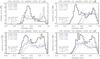 |
Fig. 8 Histograms of ratio of the intensity at the central reversal to mean intensity from peaks for the observed and synthetic profiles of the Lyα to Lyδ lines. The solid black line represents the observed data. Three values of μ are represented by corresponding colours and line-styles. |
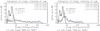 |
Fig. 9 Compared histograms of the Lyα integrated intensity of the observed profiles with those calculated using multi-thread models with hotter outer threads. Left panel: multi-thread models with T0 values of 30 000 and 15 000 K in the outer threads. Right panel: comparison for somewhat lower temperatures of 15 000 and 10 000 K. The solid black line represents the observed data. Three values of μ are represented with corresponding colours and line-styles. |
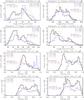 |
Fig. 10 Compared histograms of selected Lyman-line profile characteristics for synthetic profiles calculated using the models with identical threads (denoted as ident.) and models with outer threads with temperatures T0 of 9000 and 10 000 K (denoted as nidn) with histograms of characteristics of observed profiles (solid black line). |
5. Discussion
The multi-thread model with identical threads is not able to reproduce the histogram of the observed Lyα integrated intensity with two peaks. The reason for this might be that in reality threads in prominences are probably not identical. To investigate this idea, we used for the first time 2D multi-thread models with non-identical threads. We placed two hotter threads on either sides of the multi-thread model while keeping the total number of threads equal to 10. Assuming central temperatures T0 above 10 000 K in the outer threads while keeping inner threads temperature T0 at 8000 K leads to histograms of integrated intensities of the synthetic Lyα to Lyδ lines that are much wider than the observed data histograms. When using central temperatures T0 of the outer threads that are only one and two thousand K higher than in the inner threads, the histograms of the centre-to-peak ratio of the synthetic Lyα line with single peak were obtained for all three LOS angles 0°, 30° and 60° (corresponding to μ values of 1, 0.866, and 0.5). This agrees well with the observed Lyα line histogram that likewise has a single peak. In contrast, the multi-thread model with identical threads produces histograms with two-peak distribution of the Lyα centre-to-peak ratio. The histograms of the centre-to-peak ratio for the synthetic Lyβ, Lyγ and Lyδ lines differ only slightly from those obtained with the identical-thread model. However, using the hotter outer threads does not lead to histograms of integrated intensity of the synthetic Lyα profiles with two peaks as in the observed data. We also ran tests with outer threads having a lower central column mass M0. However, these models did not lead to a double-peaked distributions of the synthetic Lyα integrated intensities. For example, using M0 lower by an order of magnitude, 1 × 10⁻⁵ g cm2, in the outer threads (Model_2 of Berlicki et al.2011) only shifts the histograms of the integrated intensities and the centre-to-peak ratio to lower values. It can be also argued that the temporal changes of the prominence structure occurring during the observations cannot be the cause of the double-peak distribution of the observed Lyα integrated intensities. This is because variations of the Lyα integrated intensities between individual spectra obtained at different times are significantly smaller (lower than 40%) than the difference between the peaks in the histogram. The lower intensity peak in the histogram could be caused by the apparent spatial separation of the lower and higher intensity Lyα profiles within the spectra. The lower-intensity profiles tend to cluster in the southern part of the slit, which is probably located outside of the bright part of the observed prominence (see Fig. 1, left). However, without co-temporal high-resolution Hα observations we cannot study this spatial distribution in detail. The disagreement for histograms of the Lyα and Lyβ centre-to-peak ratio might be explained by neglecting the mutual radiative interaction between individual threads. As was shown by Heinzel et al. (2010) using 2D multi-thread models with three identical threads, the mutual radiative interaction mainly influences peaks of the Lyman-line profiles, thus mainly histograms of the centre-to-peak ratio are affected. Heinzel et al. (2010) found that the most intense profiles have the highest increase of intensities at peaks and that the influence of the mutual radiative interaction decreases with the distance between threads. Thus, with increasing intensities at peaks, the number of deeper profiles increases, while the number of shallower profiles at the same time decreases. This shifts the maxima of the centre-to-peak ratio histograms towards lower values. The effect of the mutual radiative interaction is strongest mainly for the Lyα and Lyβ lines. In contrast, Heinzel (1989) found an opposite effect for a 1D multi-thread model with 40 threads – the intensity at peaks decreased when mutual interaction was taken into account. This discrepancy between the findings of Heinzel (1989) in 1D and of Heinzel et al. (2010) in 2D geometry clearly shows that the question of the effect of the mutual radiative interaction is still unanswered. We plan to study it in detail in future with 2D multi-thread models.
6. Conclusions
We analysed the quiescent prominence observed on NW limb on May 18, 2005 in detail. Using profile-to-profile comparison of the observed Lyα profiles with the synthetic Lyα profiles obtained by the single-thread model, we found a set of input parameters representing a rather dense prominence with the central total column mass M0 ~ 10-4 g/cm2. This is similar to Model1 found by Gunár et al. (2010). For the statistical analysis we used three characteristics of the Lyman-line profiles: the integrated intensity, the Lyman decrement ratio, and the ratio of intensity at the central reversal to average intensity of peaks. The multi-thread model with ten identical threads used for this statistical analysis agrees satisfactorily with observations for histograms of the integrated intensities of synthetic and observed Lyα to Lyδ line profiles for angles 30° and 60° (corresponding to the μ of 0.866 and 0.5) between the LOS and the direction perpendicular to the magnetic field. LOS angles different from perpendicular were used here for the first time. However, the multi-thread model with identical threads is not capable to reliably reproduce the two-peaked histograms of the observed Lyα integrated intensities. In addition, while the histograms of the Lyman decrements of Lyγ/Lyβ and Lyδ/Lyβ agree very well with observations, the Lyα/Lyβ histograms of the synthetic data are considerably wider (due to the double-peak distribution of the Lyα integrated intensities) than the histograms of the observed data. Histograms of the centre-to-peak ratio for the synthetic Lyα and Lyβ lines fit the observed data only partially, while for Lyγ and Lyδ the agreement is satisfactory. Gunár et al. (2010) found for a different prominence also agreement of the centre-to-peak histograms with observations only for Lyγ and Lyδ. But the discrepancy between their Lyα and Lyβ synthetic and observed data is much more significant.
To investigate the idea that the double-peak histograms of the observed Lyα integrated intensities might be caused by threads with various plasma parameters, we used here for the first time multi-thread models with non-identical threads. When we used relatively hot threads (T0> 10 000 K) at the edges of the multi-thread model, the synthetic spectra histograms of integral intensities were significantly different from the observed data histograms. This clearly shows that a relatively large variation of parameters of multi-thread model, even in a few of the threads, produces a very large difference in the synthetic spectra. On the other hand, when we used outer threads with slightly higher temperatures (T0 = 10 000 and 9000 K), only some of the statistical parameters were significantly affected, improving the agreement with observations in several cases and deteriorating it in others. Therefore we argue that the temperature in the interiors of cool prominence fine structures in the studied prominence is at about 8000 K and does not vary significantly among individual structures. This means that the multi-thread model with identical threads is sufficient for a statistical comparison of observed and synthetic data. However, none of the multi-thread models with non-identical threads was able to reproduce the double-peak histogram of the observed Lyα integrated intensities.
The results of the multi-thread model with hotter threads at its edges does not suggest that areas with plasma of higher temperatures do not exist in prominences. The visibility of prominences in the transition-region (TR) lines was previously demonstrated by Poland & Tandberg-Hanssen (1983) on UV observations of a prominence obtained on November 20, 1980 by the Ultraviolet Spectrometer and Polarimeter (Woodgate et al. 1980) onboard the Solar Maximum Mission. For filaments, the TR O v line emission from PCTR was assumed in Schwartz et al. (2004). However, results presented here show that extended regions of prominences filled with plasma at the lower limit of PCTR temperatures (below 30 000 K) would have a significant effect on the Lyman spectra emitted by prominences.
Acknowledgments
P.S. acknowledges support from grant P209/12/0906 of the Grant Agency of the Czech Republic. S.G. acknowledges support from the European Commission via the Marie Curie Actions – Intra-European Fellowships Project No. 328138. The work of P.S. was supported by project RVO: 67985815. P.S. acknowledges support from the Slovak Research and Development Agency under the contract No. APVV-0816-11. The work of P.S. was supported by grant project VEGA 2/0108/12 of the Science Grant Agency. S.G. thanks for support by the Astronomical Institute of the Academy of Sciences of the Czech Republic. We are thankful to P. Heinzel for providing us with his 2D non-LTE code for solving radiative transfer in solar prominences. We are also thankful to the anonymous referee for useful comments and suggestions.
References
- Anzer, U., & Heinzel, P. 1998, Sol. Phys., 179, 75 [NASA ADS] [CrossRef] [Google Scholar]
- Anzer, U., & Heinzel, P. 1999, A&A, 349, 974 [NASA ADS] [Google Scholar]
- Auer, L. H., & Paletou, F. 1994, A&A, 285, 675 [NASA ADS] [Google Scholar]
- Berlicki, A., Gunár, S., Heinzel, P., Schmieder, B., & Schwartz, P. 2011, A&A, 530, A143 [NASA ADS] [CrossRef] [EDP Sciences] [Google Scholar]
- Curdt, W., Brekke, P., Feldman, U., et al. 2001, A&A, 375, 591 [NASA ADS] [CrossRef] [EDP Sciences] [Google Scholar]
- Goode, P. R., Denker, C. J., Didkovsky, L. I., Kuhn, J. R., & Wang, H. 2003, J. Kor. Astron. Soc., 36, 125 [CrossRef] [Google Scholar]
- Gouttebroze, P. 2006, A&A, 448, 367 [NASA ADS] [CrossRef] [EDP Sciences] [Google Scholar]
- Gouttebroze, P., Heinzel, P., & Vial, J. C. 1993, A&AS, 99, 513 [NASA ADS] [Google Scholar]
- Gunár, S. 2014, in IAU Symp., 300, 59 [Google Scholar]
- Gunár, S., Heinzel, P., Schmieder, B., Schwartz, P., & Anzer, U. 2007, A&A, 472, 929 [NASA ADS] [CrossRef] [EDP Sciences] [Google Scholar]
- Gunár, S., Heinzel, P., Anzer, U., & Schmieder, B. 2008, A&A, 490, 307 [NASA ADS] [CrossRef] [EDP Sciences] [Google Scholar]
- Gunár, S., Schwartz, P., Schmieder, B., Heinzel, P., & Anzer, U. 2010, A&A, 514, A43 [NASA ADS] [CrossRef] [EDP Sciences] [Google Scholar]
- Gunár, S., Heinzel, P., & Anzer, U. 2011a, A&A, 528, A47 [NASA ADS] [CrossRef] [EDP Sciences] [Google Scholar]
- Gunár, S., Parenti, S., Anzer, U., Heinzel, P., & Vial, J.-C. 2011b, A&A, 535, A122 [NASA ADS] [CrossRef] [EDP Sciences] [Google Scholar]
- Gunár, S., Mein, P., Schmieder, B., Heinzel, P., & Mein, N. 2012, A&A, 543, A93 [NASA ADS] [CrossRef] [EDP Sciences] [Google Scholar]
- Gunár, S., Schwartz, P., Dudík, J., et al. 2014, A&A, 567, A123 [NASA ADS] [CrossRef] [EDP Sciences] [Google Scholar]
- Heasley, J. N., & Mihalas, D. 1976, ApJ, 205, 273 [NASA ADS] [CrossRef] [Google Scholar]
- Heinzel, P. 1989, Hvar Observatory Bulletin, 13, 317 [Google Scholar]
- Heinzel, P. 2007, in The Physics of Chromospheric Plasmas, eds. P. Heinzel, I. Dorotovič, & R. J. Rutten, ASP Conf. Ser., 368, 27 [Google Scholar]
- Heinzel, P., & Anzer, U. 2001, A&A, 375, 1082 [NASA ADS] [CrossRef] [EDP Sciences] [Google Scholar]
- Heinzel, P., Anzer, U., & Gunár, S. 2010, Mem. Soc. Astron. It., 81, 654 [NASA ADS] [Google Scholar]
- Kunasz, P., & Auer, L. H. 1988, J. Quant. Spec. Radiat. Transf., 39, 67 [NASA ADS] [CrossRef] [Google Scholar]
- Labrosse, N., Heinzel, P., Vial, J., et al. 2010, Space Sci. Rev., 151, 243 [Google Scholar]
- Mackay, D. H., Karpen, J. T., Ballester, J. L., Schmieder, B., & Aulanier, G. 2010, Space Sci. Rev., 151, 333 [NASA ADS] [CrossRef] [Google Scholar]
- Mihalas, D., Auer, L. H., & Mihalas, B. R. 1978, ApJ, 220, 1001 [NASA ADS] [CrossRef] [Google Scholar]
- Patsourakos, S., & Vial, J.-C. 2002, Sol. Phys., 208, 253 [NASA ADS] [CrossRef] [Google Scholar]
- Poland, A., & Anzer, U. 1971, Sol. Phys., 19, 401 [Google Scholar]
- Poland, A. I., & Tandberg-Hanssen, E. 1983, Sol. Phys., 84, 63 [Google Scholar]
- Schühle, U. 2003, SUMER Data Cookbook, Published at http://www.mps.mpg.de/projects/soho/sumer/text/cookbook.html [Google Scholar]
- Schwartz, P., Heinzel, P., Anzer, U., & Schmieder, B. 2004, A&A, 421, 323 [NASA ADS] [CrossRef] [EDP Sciences] [Google Scholar]
- Schwartz, P., Schmieder, B., Heinzel, P., & Kotrč, P. 2012, Sol. Phys., 281, 707 [NASA ADS] [CrossRef] [Google Scholar]
- Wilhelm, K., Curdt, W., Marsch, E., et al. 1995, Sol. Phys., 162, 189 [NASA ADS] [CrossRef] [Google Scholar]
- Woodgate, B. E., Brandt, J. C., Kalet, M. W., et al. 1980, Sol. Phys., 65, 73 [NASA ADS] [CrossRef] [Google Scholar]
All Tables
All Figures
|
Fig. 1 Left panel: part of the full-disk Hα line-centre filtergram obtained by BBSO/NST on 18 May 2005. Vertical bar marks the position of the SoHO/SUMER slit. Spectra were obtained only from the part of the slit that is marked by the solid line because the SUMER detector was partially damaged. Right panel: prominence seen as a filament in part of the full-disk observations in the Hα line centre made at the Kanzelhöhe Solar Observatory three days earlier. The two clearly visible Hα features marked by arrows and denoted as NHS and SHS are the northern and southern Hα prominence structures. |
| In the text | |
|
Fig. 2 Calibrated spectra of the Lyα–Lyδ lines. The spectra were corrected for vertical shifts. The vertical white bar marks the usable part of the slit. |
| In the text | |
|
Fig. 3 Example of the temperature and gas-pressure distributions produced by the 2D single-thread model with the best agreement with observed spectra. The temperature step between contours is 10 000 K, that of the gas pressure is 0.02 dyn/cm2. |
| In the text | |
|
Fig. 4 Scheme of the prominence multi-thread model composed of N threads and LOS perpendicular to the magnetic field. Quantities ξ(j) represent the LOS velocities of individual threads. |
| In the text | |
|
Fig. 5 Example of fitting of a Lyα profile to estimate the influence of a blend on the three profile characteristics. Observed data are plotted with stars, while the resulting fitted profile (including blends) is plotted as a thick full line. The Voigt function fitting the profile in the wings is plotted as a thin solid line and the negative Gaussian in the profile reversal as a dashed line. The blend occurring at approximately 1025.5 Å was fitted with the Gaussian and is plotted in red. |
| In the text | |
|
Fig. 6 Compared histograms of the integrated intensities of the observed and synthetic Lyα to Lyδ line profiles. The solid black line represents the observed data. Three values of μ are represented by corresponding colours and line-styles. |
| In the text | |
|
Fig. 7 Compared histograms of the Lyman decrement of observed and synthetic Lyman-line profiles. The solid black line represents the observed data. Three values of μ are represented by corresponding colours and line-styles. |
| In the text | |
|
Fig. 8 Histograms of ratio of the intensity at the central reversal to mean intensity from peaks for the observed and synthetic profiles of the Lyα to Lyδ lines. The solid black line represents the observed data. Three values of μ are represented by corresponding colours and line-styles. |
| In the text | |
|
Fig. 9 Compared histograms of the Lyα integrated intensity of the observed profiles with those calculated using multi-thread models with hotter outer threads. Left panel: multi-thread models with T0 values of 30 000 and 15 000 K in the outer threads. Right panel: comparison for somewhat lower temperatures of 15 000 and 10 000 K. The solid black line represents the observed data. Three values of μ are represented with corresponding colours and line-styles. |
| In the text | |
|
Fig. 10 Compared histograms of selected Lyman-line profile characteristics for synthetic profiles calculated using the models with identical threads (denoted as ident.) and models with outer threads with temperatures T0 of 9000 and 10 000 K (denoted as nidn) with histograms of characteristics of observed profiles (solid black line). |
| In the text | |
Current usage metrics show cumulative count of Article Views (full-text article views including HTML views, PDF and ePub downloads, according to the available data) and Abstracts Views on Vision4Press platform.
Data correspond to usage on the plateform after 2015. The current usage metrics is available 48-96 hours after online publication and is updated daily on week days.
Initial download of the metrics may take a while.