| Issue |
A&A
Volume 577, May 2015
|
|
|---|---|---|
| Article Number | A7 | |
| Number of page(s) | 10 | |
| Section | Numerical methods and codes | |
| DOI | https://doi.org/10.1051/0004-6361/201424860 | |
| Published online | 22 April 2015 | |
An open-source, massively parallel code for non-LTE synthesis and inversion of spectral lines and Zeeman-induced Stokes profiles⋆
1
Instituto de Astrofísica de Canarias,
Avda vía Láctea S/N, 38205
La
Laguna, Tenerife
Spain
e-mail:
This email address is being protected from spambots. You need JavaScript enabled to view it.
2
Departamento de Astrofísica, Universidad de La Laguna
38205,
La Laguna, Tenerife,
Spain
3
Institute for Solar Physics, Dept. of Astronomy, Stockholm
University, Albanova University Center, 10691
Stockholm,
Sweden
4
Consejo Superior de Investigaciones Científicas,
28006
Madrid,
Spain
Received: 26 August 2014
Accepted: 16 January 2015
Abstract
With the advent of a new generation of solar telescopes and instrumentation, interpreting chromospheric observations (in particular, spectropolarimetry) requires new, suitable diagnostic tools. This paper describes a new code, NICOLE, that has been designed for Stokes non-LTE radiative transfer, for synthesis and inversion of spectral lines and Zeeman-induced polarization profiles, spanning a wide range of atmospheric heights from the photosphere to the chromosphere. The code features a number of unique features and capabilities and has been built from scratch with a powerful parallelization scheme that makes it suitable for application on massive datasets using large supercomputers. The source code is written entirely in Fortran 90/2003 and complies strictly with the ANSI standards to ensure maximum compatibility and portability. It is being publicly released, with the idea of facilitating future branching by other groups to augment its capabilities.
Key words: radiative transfer / Sun: chromosphere / Sun: photosphere / Sun: magnetic fields / polarization / Sun: abundances
The source code is currently hosted at the following repository: https://github.com/hsocasnavarro/NICOLE
© ESO, 2015
1. Introduction
The relevance of chromospheric-line diagnostics has increased dramatically in the past decade among solar scientists. This is due to (or evidenced by, depending on the point of view) very significant advances in both numerical simulations and spectropolarimetric observations. The largest instrumental projects for the next decades, the DKIST (previously known as ATST, Keil et al. 2011, 2003), the EST (Collados et al. 2010, 2013), and Solar-C (Katsukawa et al. 2012; Shimizu et al. 2011) have all been designed with chromospheric magnetometry as a top priority. Moreover, several important modern facilities such as SOLIS (Bertello et al. 2013; Pevtsov et al. 2011), Gregor (Denker et al. 2012; Soltau et al. 2012), the SST with CRISP (Scharmer et al. 2003, 2008), the DST and the Big Bear NST (Cao et al. 2013; Goode & Cao 2012), feature remarkable chromosphere-observing capabilities.
Numerical simulations of the solar atmosphere have grown notably in size, scope, and complexity (Stein 2012; Rempel & Schlichenmaier 2011). A particularly noteworthy effort in this context is the development of numerical MHD simulations of the magnetic chromosphere (Khomenko et al. 2014; Gudiksen et al. 2011).
Bridging the gap between the new ground-breaking observations and simulations requires complex modeling and diagnostic tools. NICOLE is a step in this direction. Capable of non-LTE (hereafter NLTE) spectral line calculations, it is suitable for the analysis of chromospheric lines and their polarization profiles in the Zeeman regime. The user is able to synthesize spectral profiles from large simulation datacubes, allowing a direct comparison with observations (it is possible to include the instrumental profile in the calculation). Conversely, the code inversion engine is able to work on the observed spectral data to infer relevant atmospheric parameters (such as temperatures, magnetic field vector, or Doppler velocities), which may provide interesting information or be compared directly with the simulations. Other existing NLTE codes that share some (but not all) of NICOLE’s features are MULTI (Carlsson 1986), RH (Uitenbroek 2001), Phoenix (Hauschildt & Baron 2006), HAZEL (Asensio Ramos et al. 2008), and PORTA (Štěpán & Trujillo Bueno 2013).
NICOLE has been designed from the beginning to work on massive datasets, for example, large simulation snapshots or high-resolution observations. The code implements a simple but efficient master-slave scheme using the widely available message-passing interface (MPI) parallelization. This design makes it suitable for any architecture, including the most powerful supercomputers with over a thousand processors. With its 1.5D approach (meaning that each model column is treated as a horizontally infinite atmosphere), almost ideal paralellization is achieved even for the largest number of processors.
The discussion presented in this section has thus far been only focused on solar physics, but this tool is of great potential usefulness in other areas of astrophysics as well. The code can easily provide flux-calibrated spectra of late-type stars. The capability for inverting stellar spectra has been implemented following the work of Allende Prieto et al. (1998, see also 2000, 2001) and works similarly to their code MISS. Chemical abundances may also be inverted using NICOLE, which might be an interesting capability for studies of solar/stellar compositions.
NICOLE has been released to the community as an open-source project under the GPL license1, which means that it may be copied, altered, and redistributed, as long as any resulting product is also distributed openly to the community. Users are welcome, and in fact encouraged, to branch out their own version of NICOLE to improve it, augment it, or to implement new features.
2. Code description
The source code is strictly compliant with Fortran 90 ANSI, except for the fact that it uses a few advanced features from the 2003 standard. This means that it is guaranteed to compile in any standard Fortran 2003 compiler and will also work with most Fortran 90 compilers (since most of them support the relevant 2003 extensions). Two external Python scripts facilitate compilation and execution to make the code as user-friendly as possible. In particular, all the user interaction is made by a Python wrapper that parses the configuration files, detects errors, and provides usage suggestions. The Fortran code works exclusively with low-level machine-produced files.
Although NICOLE has been almost entirely written from scratch and incorporates many novel modules and elements, it builds upon previous experience with other very popular radiative transfer codes. The structure of the inversion mode in NICOLE is similar to that of SIR (Stokes inversion based on response-functions, Ruiz Cobo & del Toro Iniesta 1992). In the NLTE module, the structure and variable naming is similar to MULTI (Carlsson 1986), as is the model atom file format. The numerical formulae for computing collisional rates and other details were adapted from MULTI to facilitate porting of atomic models and data. The NLTE iterative core is an implementation of the method described in Socas-Navarro & Trujillo Bueno (1997). The inversion module works in the same way as the code of Socas-Navarro et al. (1998, 2000). The following is a list of the approximations and limitations that have driven the design of NICOLE:
-
Statistical equilibrium: the NLTE atomic populations are computed assuming instantaneous balance between all transitions going into and out of each atomic level. Effects such as time-dependent ionization are thus neglected in the synthesis (although it could have been previously incorporated in the computation of the model atmosphere in the synthesis mode). The tests presented in de la Cruz Rodríguez et al. (2012) support the validity of this assumption in a realistic scenario involving the inversion of Ca ii lines. Furthermore, Leenaarts et al. (2012) pointed out that it also is a suitable strategy for Hα synthesis, provided that the MHD model accounts for such time-dependent ionization. Nevertheless, there might be other situations in which this approximation would be less adequate.
-
Complete angle and frequency redistribution (CRD): this approximation states that the frequency and direction of an emitted photon is independent of the frequency and direction of a previously absorbed photon by the atomic system. Uitenbroek (1989) demonstrated that this approximation works very well for the Ca ii infrared triplet lines. Other lines, such as Ca ii H and K, exhibit some significant discrepancies near the core, between CRD and full computations.
-
Polarization induced by the Zeeman effect: NICOLE does not account for polarization produced by scattering processes or modified by the Hanle effect. It is therefore more suitable for application on Stokes I and V, and for all the Stokes profiles only when the magnetic field is strong enough (typically in active regions).
-
Field-free NLTE populations (Rees 1969): the statistical equilibrium equations are solved neglecting the presence of a magnetic field. This is usually a good approximation (Trujillo Bueno & Landi Degl’Innocenti 1996; Bruls & Trujillo Bueno 1996).
-
Hydrostatic equilibrium: this approximation is only employed in inversion mode and only for computing the density scale. It mostly affects the conversion of optical-to-geometrical depth and, to some extent, the background opacities. Otherwise, strong line profiles are usually rather insensitive to density and pressure changes.
-
Blends: spectral calculations (both syntheses and inversions) may include an arbitrary number of lines with the only limitation that all the NLTE lines must be of the same element. Line blends are treated consistently in the final formal solution, including their polarization profiles. However, the NLTE atomic level populations are computed without considering blends. An important limitation arising from this simplification is that it is currently not possible to properly take into account the influence of an overlapping continuum transition treated in detail on the populations of a given line transition, even if both transitions are from the same species and included in the model atom.
-
Collisional damping: the code incorporates the classic Unsold formula (Unsold 1955) and the more recent formalism of Anstee & O’Mara (1995) and Barklem et al. (1998).
-
1.5D calculation: although the code works with 3D datacubes, each column is treated independently, as if it were infinite in the horizontal direction. This approximation works well in LTE and when computing some strong NLTE lines. The reason for the latter is that the opacity in the line core is so high that the photons have a short mean free path. Therefore, the populations are controlled by the environmental conditions in their immediate surroundings. Of course, this argumentation is not universal because scattering will still tend to couple distant points, and depending on its relative importance, 3D effects will be more or less relevant. A more quantitative assessment of this approximation for the inversion of the Ca infrared triplet has been presented in de la Cruz Rodríguez et al. (2012). Other investigations of 3D effects in forward modeling for various important lines have been presented in Leenaarts et al. (2009, 2012, 2013).
-
Hyperfine structure: lines with hyperfine structure may be seamlessly integrated in the spectral synthesis or inversion, simply by supplying the appropriate atomic data in the configuration file. However, this mode usually has a significant effect on the performance (e.g., Socas-Navarro, in prep.).
-
Flexible node location: the inversion nodes for NICOLE may be specified manually by the user and do not need to be equispaced. This enables a more efficient distribution of nodes through the atmosphere, packing them more densely where more information is available and spreading them out in areas where the observations are less sensitive.
-
Bezier-interpolant formal solvers: NICOLE implements a number of options for the formal solution method. A very interesting new routine is based on Bezier interpolation and makes the code more robust and stable. More details are provided in Sect. 5.1 below.
3. Equation of state
The equation of state (EoS) establishes one or more constraints that relate the various fundamental parameters defining the state of the plasma. Solving the EoS to determine physical variables, such as electron pressure, internal energy or the H− negative ion density, to name a few examples, is often a necessary intermediate step in a broad range of numerical codes for radiative transfer or MHD simulation. It is not trivial to solve the EoS when partial ionization and molecule formation are considered.
For the purposes of the calculations involved in NICOLE, the plasma state is defined by its temperature (T), gas density (ρ), gas pressure (Pg), electron pressure (Pe), and the following number densities, needed for the background opacities: neutral hydrogen atoms (H), protons (H+), negative hydrogen ions (H−), hydrogen molecules (H2), and ionized hydrogen molecules (H ). All of these parameters may be supplied as input if desired. Alternatively, one could supply two of them (temperature plus one of density, gas pressure, or electron pressure), and NICOLE will use the EoS to solve for the rest. If the option to impose hydrostatic equilibrium is set, then only the temperature stratification and the upper boundary condition for the electron pressure are needed. This is how the code works in inversion mode.
In NICOLE the solution of the EoS is divided into two, generally independent, steps. The first step computes the distribution of the various H populations (H, H+, H−, H2, and H). The second step deals with the relationship among the thermodynamical parameters (T, ρ, Pg and Pe). In both cases there are three different methods to solve the EoS in NICOLE that the user may choose from.
3.1. Full ICE solution
To determine the density of particles in the solar plasma, we need to solve not only the atomic ionization system, but also the chemical equilibrium among all the possible molecules. NICOLE implements the instantaneous chemical equilibrium (ICE) calculation of Asensio Ramos et al. (2003), Asensio Ramos & Socas-Navarro (2005), with a compilation of data for a total of 273 molecules. Obviously, dealing with such a large number of molecules results in a very demanding computation at each gridpoint, having to solve a nonlinear system of 273 equations and unknowns. In addition to the computing time demanded by this approach, there is also the problem that the iteration sometimes fails to converge. Only a very small percentage of the points suffer this convergence problem, but nevertheless, it might still be problematic for some applications in which stability over a large number of calculations is a strict requirement. Therefore, two other options, faster and more stable, have been implemented as well.
3.2. Restricted ICE solution
This is basically the same as the full solution, except that only two H molecules are considered, H2 and H. The calculation is then faster and more stable than the full ICE, but it might still fail (albeit rarely) and is slower than the NICOLE option (see below).
3.3. NICOLE method
We have developed a new procedure that avoids iteration and is therefore perfectly stable and faster than the previously discussed options. It is based on the realization that one only needs to know how much of the H is in molecular form to derive all other relevant parameters in a straightforward manner. We trained an artificial neural network (ANN) using a large database of (T, Pe, m) values for which we had previously solved the full ICE system with the 273 molecules. The third input parameter m characterizes the plasma metallicity (in a logarithmic scale), so that all elements heavier than Z = 2 have their abundances scaled by this factor. The ANN and the algorithms are very similar to those described in Socas-Navarro (2003, 2005). The training set was initially computed starting from a uniform distribution of T (between 1500 and 10 000 K), m (between −1.5 and 0.5) and log (Pg) (between −3 and 6 with Pg in dyncm-2). We used this initial dataset to study some properties of the distribution, but the actual ANN training was made using a better suited set, as explained below.
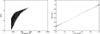 |
Fig. 1 Left: points in our initial training set that exhibit a number fraction of molecular H greater than 0.1 and smaller than 0.9. Right: scatter plot showing the accuracy of the ANN trained to retrieve the fraction of atomic H from (T, Pe and m). The standard deviation is ~5 × 10⁻³. |
Not surprisingly, the fraction of molecular H does not cover the entire parameter space in a uniform manner. Instead, it is saturated in large regions of the space, and there is only a relatively narrow range of input values in which we need to perform the calculation. This can be seen in Fig. 1 (left), which shows the (T, Pe) space spanned by the training set. The populated region has values for which the fraction of molecular H is non-trivial. The empty space to the right is too hot for molecules to form, and therefore all H is in atomic form. To the left, there are no (T, Pe) values consistent with our (T, Pg) distribution.
The results shown in Fig. 1 (left panel) suggest that we do not need to train the ANN to operate in the full domain of the input parameters. We only need to cover the populated region seen in the figure. In this manner, we not only decrease the required size of the training set but also improve the accuracy of a given ANN since it can become more specialized by operating on a smaller subspace. We therefore constructed a new better suited training set that only includes points in the relevant range. After successfully training the ANN with these points, we reached an accuracy (measured as the standard deviation of the difference between the validation set and the ANN result) of ~5 × 10⁻³ (see right panel of Fig. 1). Our ANN has four nonlinear layers with ten neurons per layer.
Once we know how much H is in the form of molecules, we use the Saha ionization equation to compute all the relevant populations. We stress that, even though this method only yields the abundance of the H molecule, it has been computed taking into account all others with the full ICE procedure.
For the thermodynamical variables we have the options described in the next sections.
3.4. The Wittman procedure
The first option is the method of Wittmann (1974), which in turn is an improvement of the method introduced by Mihalas (1974). This is the method implemented in the SIR code of Ruiz Cobo & del Toro Iniesta (1992). Only H molecules are considered here, which removes the necessity for iterations and speeds up the computation of the total gas pressure Pg. With this procedure, Pg is obtained directly from the pair of values (T, Pe). The reverse process, that is, obtaining Pe from (T, Pg), requires iteration from an initial guess, which is slower and might fail to converge. This method is a good approximation in most conditions, except for very cool plasmas, such as those in a sunspot umbra, where other molecules might be important.
3.5. Artificial neural networks
It is possible to train a set of ANNs to solve for both Pe from (T, Pg) and Pg from (T, Pe). However, this calculation is far less accurate than calculating the H molecular fraction explained above (at least using a similar sized ANN). Figure 2 shows the spread in the validation set. The error in the logarithm of the retrieved pressure is on the order of 15%. On the other hand, there are many applications in which an accurate solution of the EoS is not required, since spectral lines are far less sensitive to density or gas pressure than they are to temperature. If the penalty in accuracy is acceptable, then this method is by far the fastest and provides a direct solution in both directions.
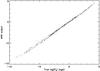 |
Fig. 2 Scatter plot showing the accuracy of the ANN trained to retrieve the logarithm of Pe from from (T, Pg and m). The standard deviation is ~15%. |
3.6. The NICOLE EoS
This is essentially the same procedure as the NICOLE method described above, using an ANN to determine the fraction of molecular H, but then solving the Saha ionization equation for the rest of atomic species to determine the electron number densities. The reverse process, that is, obtaining Pg from (T, Pe), is made by iteration, just as in the Wittmann procedure.
4. Background opacities
Background opacities result from continuum absorption processes, typically atomic photoionization. We distinguish two distinct wavelength regimes that are treated differently: ultraviolet and visible/infrared. The transition between these two regimes is located at 400 nm.
4.1. Visible and infrared opacities
NICOLE contains three different opacity packages to calculate background opacities in the visible and infrared. They account for almost the same physical processes (with the slight differences that we detail below) and therefore mostly differ in details such as the tabulated values employed or the actual coding.
4.1.1. The Wittmann package
This package computes continuum opacities due to H−, neutral H, He−, H , H
, H , photoionization of Ca, Na and Mg, and Rayleigh scattering by neutral H, H2, neutral He and Thomson scattering by electrons. For more details see Wittmann (1974).
4.1.2. The SOPA package
We implemented a module with the background opacity package of Kostik et al. (1996), which includes neutral H, H−, H, photoionizations from the first eight levels of Si, C, Mg, Al, and the first two levels of Fe, Rayleigh scattering by neutral H and Thomson scattering by free electrons. Unfortunately, we were not able to bring this package to the coding standards of the NICOLE requirements. To avoid compile problems or hardware incompatibilities, this package is not supported. It is disabled by default and available only by a special compilation-time switch for advanced users.
4.1.3. The NICOLE package
We developed an independent opacity package for NICOLE that computes opacities from neutral H, H− and Mg, as well as scattering due to H, H2 and free electrons.
Figures 3 and 4 compare the wavelength dependence of the background opacities computed by all three packages. Since this comparison strongly depends on the atmospheric conditions, we have chosen two sets of parameters.
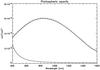 |
Fig. 3 Background opacities as a function of wavelength in typical photospheric conditions (T = 5600 K, Pe = 10 dyn cm-2, Pg = 8 × 10⁵ dyn cm-2). Solid line: using the Wittmann package. Dashed line: using the NICOLE package. Dotted line: using the SOPA package. The lower curve represents the scattering contribution to the opacity (all three packages yield the same result within the line thickness of the plot). The scattering curve has been multiplied by a factor 100 for better visibility in this plot. |
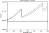 |
Fig. 4 Background opacities as a function of wavelength in typically chromospheric conditions (T = 9000 K, Pe = 0.05 dyn cm-2, Pg = 0.15 dyn cm-2). Solid line: using the Wittmann package. Dashed line: using the NICOLE package. Dotted line: using the SOPA package. The lower curve represents the scattering contribution to the opacity (all three packages yield the same result within the line thickness of the plot). |
4.2. Ultraviolet opacities
Computating background opacities in the ultraviolet is far more complicated than in the visible. Many metallic species can undergo photoionization processes with sufficiently large cross-sections to become important opacity contributors in spite of their relatively low abundances. To complicate the matter further, there is no dominant species above the 91 nm regime, where the H photoionization occurs. Depending on the prevailing conditions and the wavelength range, different metals dominate. In addition to the SOPA package (see above), which includes some photoionization processes for a few interesting metals, we have two other packages in NICOLE that are specifically implemented to compute ultraviolet opacities.
4.2.1. The Dragon-Mutschlecner package
Dragon & Mutschlecner (1980) provided a set of tables to compute photoionization cross-sections for various levels of neutral Mg, Al, Si, and Fe. Using some simple analytical expressions, we can obtain a rather good approximation in most practical situations (see Figs. 5 and 6 below).
4.2.2. The TIP-TOP package
The Iron Project (TIP) and The Opacity Project (TOP) are two large collaborations aimed at producing the most comprehensive compilation of atomic opacity sources. The two projects began as independent initiatives, but have now joined forces and have published their tables with a large number of photoionization cross-sections for most metals. We have included all the available data for neutral and singly ionized elements between Z = 1 and Z = 26. In the particular case of the Fe atom, we use the data provided by Bautista (1997) and by Nahar & Pradhan (1994). In all cases the data are smoothed as discussed in Bautista et al. (1998), Allende Prieto et al. (2003), Allende Prieto (2008).
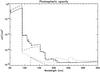 |
Fig. 5 Ultraviolet background opacities as a function of wavelength in typical photospheric conditions (T = 5600 K, Pe = 10 dyn cm-2, Pg = 8 × 10⁵ dyn cm-2). Solid line: using the TIP-TOP package. Dashed line: using the Dragon-Mutschlecner package. Dotted line: using the SOPA package. The lower dashed curve represents the scattering contribution to the opacity (all three packages yield the same result within the line thickness of the plot). |
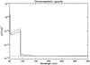 |
Fig. 6 Ultraviolet background opacities as a function of wavelength in typical chromospheric conditions (T = 9000 K, Pe = 0.05 dyn cm-2, Pg = 0.15 dyn cm-2). Solid line: using the TIP-TOP package. Dashed line: using the Dragon-Mutschlecner package. Dotted line: Using the SOPA package. The lower dashed curve represents the scattering contribution to the opacity (all three packages yield the same result within the line thickness of the plot). |
To make the problem tractable, NICOLE preloads in memory a large matrix with all the cross-sections (for each element and level) at each wavelength, discretized with a 0.1 nm sampling. When the opacity routine is called for a certain wavelength and input conditions, the code simply picks from the matrix all the cross-sections at that wavelength (rounded to the closest point in the grid), weighs each one according to element abundance, ionization fraction, and level excitation, and finally returns the total of all the contributors. With this strategy, we can obtain the total opacity from all contributors in the comprehensive TIP-TOP database in a very short time.
Figures 5 and 6 compare the various ultraviolet opacity packages in two different situations. In the photosphere (Fig. 5), the TIP-TOP package yields a much more detailed curve with a plethora of peaks and discontinuities caused by photoionization from countless levels of several elements. The other two packages, however, produce a good smoothed-out approximation. Under these atmospheric conditions, the opacity is dominated by neutral species. Under the chromospheric conditions of Fig. 6, the opacity structure is much simpler. It is dominated by Thomson scattering on free electrons at all but the shortest wavelengths. Under these conditions we begin to find some non-negligible contributions from ionized metals.
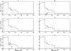 |
Fig. 7 Contribution of the most relevant metals to the background ultraviolet opacity in typical photospheric conditions (T = 5600 K, Pe = 10 dyn cm-2, Pg = 8 × 10⁵ dyn cm-2). Other elements become relevant under different conditions. Solid: total opacity from all neutral and singly ionized elements between Z = 1 and Z = 26. Dotted: resulting opacity when neglecting all metals except for the one indicated in the title of each plot. |
Figure 7 shows the relative contribution of several important elements to the total UV background opacity under typical photospheric conditions. The computation is based on the detailed TIP-TOP photoionization data, considering all neutral and singly ionized elements up to Fe.
Sometimes it is necessary to have some means to account for the line blanketing effect, that is, the concentration of very many spectral lines that act similarly to a continuum opacity source. In our code this is accomplished in practice by using “fudge factors” that may be configured in the input file independently for each one of the spectral regions defined.
5. Formal solutions
Inside each vertical column, NICOLE solves the NLTE problem in 1D by assuming plane-parallel geometry, isotropic scattering, and complete frequency redistribution (details in Socas-Navarro & Trujillo Bueno 1997). To compute the atom population densities, the code assumes statistical equilibrium and unpolarized light. When the populations are known, the full-Stokes vector is computed for Zeeman-induced polarization. Therefore, all Zeeman sublevels originating from a given atomic level are assumed to be equally populated, discarding any quantum interference between them (Trujillo Bueno & Landi Degl’Innocenti 1996).
5.1. Formal solutions and the NLTE problem
The radiative transfer equation for unpolarized light can be expressed as 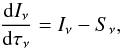 (1)where Iν is the emerging intensity at frequency ν, τν is the optical depth, and Sν is the source function. In a discrete grid of depth points where the subindexes u, o and d indicate the upwind point, central point, and downwind point, the solution to Eq. (1) on the interval (τo,τu) is
 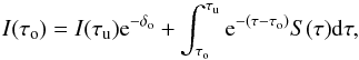 (2)where δo ≡ δτo = | τu − τo |. To analytically integrate Eq. (2), the source function can be approximated using a polynomial interpolant: linear, quadratic, etc. We have implemented two formal solutions of the radiative transfer equation (methods) to compute the atom population densities (unpolarized), based on short-characteristics:
-
1.
The source function is approximated with a parabolic interpolant, centered on the grid point at which the intensity is calculated (Olson & Kunasz 1987). This interpolant behaves particularly well on equidistant grids, but it is known to overshoot on irregular grids. Therefore, when overshooting is detected, we instead adopt a linear approximation.
-
2.
An elegant approach, introduced by Auer (2003), is to use Bezier-splines interpolants. Bezier-splines provide a powerful framework to control overshooting while keeping the accuracy of high-order interpolants. These methods have been implemented in 3D MHD codes (e.g., BIFROST, Hayek et al. 2010) and radiative transfer codes (e.g., Multi3d, PORTA, Leenaarts & Carlsson 2009a; Štěpán & Trujillo Bueno 2013).
In particular, we have experimented extensively with the election of an appropriate diagonal approximate lambda operator and the treatment of overshooting cases in method 2. The quadratic Bezier interpolant is defined using normalized abscissa units in the interval (xo,xu)  which means that
  (3)where C is a control point defined as
  (4)The solution to Eq. (2) can be formulated in two ways. One is to re-arrange the terms of the integral so we derive terms that only depend on the values of the source function in the upwind point (u), downwind point (d), and central point (o) by explicitly replacing Eq. (4) into Eq. (3) before the integral in Eq. (2) is performed,
 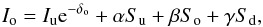 (5)where α,β,andγ are the interpolation coefficients. This was the choice of Hayek et al. (2010), therefore they chose an expresion to numerically compute dS0/ dτ , which linearly depends on Su,So,andSd. However, de la Cruz Rodríguez & Piskunov (2013) and Štěpán & Trujillo Bueno (2013) expressed the solution as a function of Su,So,andC:
  (6)In principle, the two formalisms should be equivalent. The only difference appears when the diagonal approximate lambda operator is computed (details in Olson & Kunasz 1987). To define the approximate lambda operator, one can use a source function that is set to zero at all depth points except So = 1 and check which terms remain in Eqs. (5) and (6). Note that we are strictly neglecting the contribution from the ensuing intensity through the term Iue− δo, which is typically very small in the optically thick regime (van Noort et al. 2002).
The implementation by Hayek et al. (2010) implicitly includes the terms used to compute dS0/ dτ in their operator, whereas the second formalisms does not. It is straightforward to see that these terms appear because the derivative is computed numerically, but there is no reason to include them in the approximate operator. In addition, by using the second formalism, it does not matter so much what expresion is used for the derivative, given that the control point is not explicitely split into terms that depend on Sd, So , and Su (Auer 2003, proposed two different ways of computing centered derivatives). Our tests show that defining the local operator as  is optimal and convergence is achieved in fewer iterations.
Overshooting is suppressed by changing the value of the control point C as described in Hayek et al. (2010). The basic idea is to identify extrema in the source function and to constrain the value of the control point within Su and So. An important refinement was proposed by Štěpán & Trujillo Bueno (2013), who also investigated overshooting in the downwind interval between So and Sd. The latter indeed improves the stability of the solution, forcing the Bezier interpolant to approach point o monotonically in every situation.
So far, we have not considered method 1 in any great detail. The problem is that allowing the solution to switch from parabolic to linear and vice versa can lead to a flip-flop behavior. Normally, more iterations are needed to reach a similar convergence threshold with this method than with the Bezier alternative.
5.2. Formal solution of the polarized transfer equations
When the level populations are calculated, NICOLE allows computing the emerging Stokes vector assuming Zeeman-induced polarization. We have implemented a list of formal solvers that can be used for this matter. The following alternatives are available:
-
Quadratic and cubic DELO-Bezier (de la Cruz Rodríguez & Piskunov 2013);
-
DELO-linear (Rees et al. 1989);
-
DELO-parabolic (Trujillo Bueno 2003);
-
Hermitian (Bellot Rubio et al. 1998);
-
Weakly polarizing media (Sánchez Almeida & Trujillo Bueno 1999).
6. Hyperfine structure
Almost every element in the periodic table has an isotope with nonzero nuclear angular momentum I, which is coupled with the sum of the orbital and spin angular momentum J. Consequently, the fine structure levels, characterized by their value of J, are split into hyperfine structure levels following the standard rule for angular momentum addition, yielding F = | J − I | ...J + I. The hyperfine splitting is usually much weaker than the fine-structure splitting. Thus, a weak magnetic field may be able to produce Zeeman splittings that are on the order of the energy level separation between consecutive F levels. Under these circumstances, the nondiagonal terms in the Zeeman Hamiltonian become important. This regime of intermediate Paschen-Back effect (or Back-Goudsmit effect) leads to strong perturbations on the Zeeman patterns, which may have a strong impact on the emerging Stokes profiles.
The energy splitting of these F levels with respect to the original J level (the fine-structure level without hyperfine structure) was given, with very good approximation, by Casimir (1963):  (7)where
  (8)The energy splitting is represented in cm-1 when the constants A and B are given in cm-1. These constants are the magnetic-dipole (A) and electric-quadrupole (B) hyperfine structure constants and are characteristic of a given fine structure level. If the energy level separation between consecutive fine structure levels is much larger than the typical Zeeman splitting produced by the magnetic fields we are interested in, one may focus exclusively on the coupling between the hyperfine and magnetic interactions. The total Hamiltonian is block-diagonal, and each block can be written as (e.g., Landi Degl’Innocenti & Landolfi 2004)
  (9)where μ0 is the Bohr magneton, B is the magnetic field strength, and gJ is the Landé factor of the level in L-S coupling.
The total Hamiltonian is diagonal in MF, so that it remains a good quantum number even in the presence of a magnetic field. This is not the case for F because the total Hamiltonian mixes levels with different values of F. After a numerical diagonalization of the Hamiltonian, the eigenvalues are associated with the energies of the MF magnetic sublevels. The transition between the upper and lower fine-structure levels produce many allowed transitions following the selection rules ΔMF = 0, ± 1. The strength of each component can be obtained by evaluating the squared matrix element of the electric dipole operator (Landi Degl’Innocenti & Landolfi 2004),  (10)where
 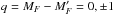 and | (LS)JIiMF ⟩ are the eigenvectors of the Hamiltonian. The symbol i is used for identification purposes since F is not a good quantum number (e.g., Landi Degl’Innocenti & Landolfi 2004).
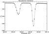 |
Fig. 8 Simulated inversion of three element abundances: O, Ni and Sc. |
7. Abundance inversions
When working in inversion mode, it is possible to set element abundances as “inversion nodes”. In this manner, NICOLE can be used in studies of solar and stellar chemical compositions, similarly to the MISS code of Allende Prieto et al. (2001). In principle, it is possible to simultaneously invert abundances and atmospheric parameters. However, it is important to realize that this would only produce meaningful results if the observations include lines from multiple elements that can univocally constrain both the atmosphere and the composition. In general, it is better to have independent observations to determine the atmospheric model, or at least to have a good approximation to it before attempting to invert abundances.
Figure 8 shows a simulated inversion of the well-known blend of Ni i with a forbidden O i transition at 6300.3 Å along with the nearby Sc ii line. These lines have frequently been used in recent studies of the solar chemical composition because this region has proven to be a valid diagnostics to resolve the so-called solar oxygen crisis (e.g., Socas-Navarro, in prep. and references therein). The simulated observations were synthesized with the HSRA quiet-Sun model (Gingerich et al. 1971), adding random noise of a 1σ amplitude of 5 × 10⁻⁴. The reference abundances chosen in this test for the lines in the figure are 8.83, 6.25, and 3.17 (O, Ni, and Sc, respectively). The inversion was initialized with highly discrepant values, 8.00, 5.50, and 4.00, and was repeated up to 30 times adding a random perturbation of up to ±0.2 dex to the reference values. Only 8 out of the 30 inversions converged to the correct solution, producing a fit down to the noise level. The fit shown in the figure is representative of these eight solutions and has a χ2 value that is approximately that of their average. The mean value and standard deviation of the results from the inversions are 8.835 ± 0.004, 6.254 ± 0.004, and 3.174 ± 0.004, respectively.
It is important to note that these extremely small uncertainties only represent the inversion error. In this case, the model atmosphere is prescribed and known a priori because we are interested here in the error produced by the inversion process and in the abilitly of the algorithm to find the correct solution. Otherwise, systematic errors would also arise from the atmospheric model uncertainty; they would probably be much larger.
8. Parallelization
NICOLE was designed to work on large datasets, typically inversions of spectral (or, in general, spectropolarimetric) scans of a 2D field of view (de la Cruz Rodríguez et al. 2013b) or spectral synthesis in simulation datacubes (Socas-Navarro, in prep.). For these applications, an efficient parallelization scheme is required.
NICOLE operates in the so-called 1.5D regime, where the radiative transfer problem is independently solved for each column. Therefore, parallelization is much easier than for 3D (see Leenaarts & Carlsson 2009b; Štěpán & Trujillo Bueno 2013). Our scheme is similar to the recent version of MULTI_3D, but we implemented a master-slave approach in which each slave works on a given spatial pixel. All input and output tasks are handled by the master process, which reads the input files, sends the input data to each idle slave, collects the computation results, and finally writes them to disk. This strategy eliminates possible disk access conflicts or bottlenecks among processes and is best suited to minimize the computing time for complex problems. We achieve the goal of ideal parallelization, in which the CPU time is inversely proportional to the number of processors (as long as the computation time is much longer than the time it takes to read the input data). This ideal parallelization holds independently of the number of processors, making NICOLE a massively parallel code that is expected to run efficiently even on the largest supercomputers with thousands of processors. We present some tests below that demonstrate this good behavior for up to 200 processors.
We conducted a series of tests with a benchmark calculation using the 3D MHD model computed with the BIFROST code (see Gudiksen et al. 2011). The snapshot used in our calculations is snapshot 385 from the “en024048_hion” simulation, which is publicly available as part of the Interface Region Imaging Spectrograph (IRIS, De Pontieu et al. 2014) mission data (full description in Carlsson 2013). This simulation snapshot has previously been used in several studies (e.g., Leenaarts et al. 2012; de la Cruz Rodríguez et al. 2013a; Pereira et al. 2013). The simulation is computed on a grid of (x, y, z) = 504 × 505 × 496 points, corresponding to a physical size of approximately 24 × 24 Mm in the (x, y)-plane. Vertically, the simulation extends from 2.2 Mm below the photosphere to 15 Mm above, and it encloses a photosphere, chromosphere, and corona. We only considered every fourth pixel in the horizontal (x, y)-plane to be able to perform the calculation with a reduced number of CPUs in our tests.
For each column in the simulation, we solved the NLTE problem with a six-level Ca ii atom and computed intensity and polarization profiles in the 8542 Å line. The hardware platform was a Linux AMD Opteron cluster with 524 cores. We employed a homogeneous subset of 204 cores in our tests (this cluster has several different processor models). Figure 9 shows a log-log plot of the total CPU time versus the inverse of the number of (slave) processors employed. In the ideal case of optimal paralellization, a straight line with a slope of −1 is expected, whose abscissa at origin is the number of columns multiplied by the computing time per column. The figure shows that the tests follow this ideal behavior (represented by the dashed line), without signs of saturation even at 200 processors.
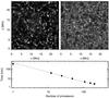 |
Fig. 9 Top row: synthetic observations in the 854.2 nm line, close to line center (left panel) and in the extended photospheric wing (right panel). Bottom: CPU time as a function of the inverse number of processors. The dotted line represents the behavior expected for ideal parallelization. |
Our parallelization is implemented using the MPI library. It is straightforward to compile and run the parallel version of NICOLE on any system with a working MPI installation. Since one of the processes is the master, it is usually more efficient to run NICOLE with N + 1 threads, where N is the number of available hardware processor cores.
9. Conclusions
NICOLE is the result of many years of effort to produce a public, well-documented, user-friendly code for massive radiative transfer calculations. It may be used in LTE or NLTE to convert atmospheric models between geometrical and optical depth or to invert observed profiles. It may be applied to solar or stellar models and observations. Interested researchers are invited to download the code from the link above and are encouraged to make and redistribute any changes or modifications they deem necessary (permissions are explicitly granted under the GNU public license).
We expect that codes such as NICOLE will become an important tool in the coming years, at least within the solar community. The advent of new instrumentation designed for chromospheric magnetometry will produce enormous datasets of NLTE spectral profiles that will require inversion. Additionally, state-of-the-art 3D numerical simulations of the solar atmosphere, spanning the whole range from the photosphere to the transition region, are becoming available and are increasingly realistic. Polarized spectral synthesis in the simulation datacubes are necessary for the detailed comparison between simulations and observations.
NICOLE has already been tested, and publications exist that demonstrate its performance in inverting Stokes profiles in LTE (Socas-Navarro 2011), NLTE (de la Cruz Rodríguez et al. 2012, 2013b; Leenaarts et al. 2014), and in synthesizing large numbers of profiles in 3D atmospheric models (Socas-Navarro, in prep.).
A significant fraction of the NICOLE development effort has been directed to making this code as user-friendly as possible. However, it is important to remember that NICOLE, like any other complex numerical code, cannot be used as a black box. Understanding not only the underlying physics, but also the numerical procedures and the data products involved, is of paramount importance to obtain meaningful scientific results.
Acknowledgments
The authors thankfully acknowledge the technical expertise and assistance provided by the Spanish Supercomputing Network (Red Española de Supercomputación), as well as the computer resources used: the LaPalma Supercomputer, located at the Instituto de Astrofísica de Canarias. Financial support by the Spanish Ministry of Science and Innovation through project AYA2010-18029 (Solar Magnetism and Astrophysical Spectropolarimetry) is gratefully acknowledged. A.A.R. also acknowledges financial support through the Ramon y Cajal fellowship.
References
- Allen de Prieto, C. 2008, Phys. Scr. T, 133, 014014 [NASA ADS] [CrossRef] [Google Scholar]
- Allende Prieto, C., Ruiz Cobo, B., & García López, J. 1998, ApJ, 502, 951 [NASA ADS] [CrossRef] [Google Scholar]
- Allende Prieto, C., García López, R. J., Lambert, D. L., & Ruiz Cobo, B. 2000, ApJ, 528, 885 [NASA ADS] [CrossRef] [Google Scholar]
- Allende Prieto, C., Barklem, P. S., Asplund, M., & Ruiz Cobo, B. 2001, ApJ, 558, 830 [NASA ADS] [CrossRef] [Google Scholar]
- Allen de Prieto, C., Lambert, D. L., Hubeny, I., & Lanz, T. 2003, ApJS, 147, 363 [NASA ADS] [CrossRef] [Google Scholar]
- Anstee, S. D., & O’Mara, B. J. 1995, MNRAS, 276, 859 [NASA ADS] [CrossRef] [Google Scholar]
- Asensio Ramos, A., & Socas-Navarro, H. 2005, A&A, 438, 1021 [NASA ADS] [CrossRef] [EDP Sciences] [Google Scholar]
- Asensio Ramos, A., Trujillo Bueno, J., Carlsson, M., & Cernicharo, J. 2003, ApJ, 588, L61 [NASA ADS] [CrossRef] [Google Scholar]
- Asensio Ramos, A., Trujillo Bueno, J., & Landi Degl’Innocenti, E. 2008, ApJ, 683, 542 [NASA ADS] [CrossRef] [Google Scholar]
- Auer, L. 2003, in Stellar Atmosphere Modeling, eds. I. Hubeny, D. Mihalas, & K. Werner, ASP Conf. Ser., 288, 3 [Google Scholar]
- Barklem, P. S., Anstee, S. D., & O’Mara, B. J. 1998, PASA, 15, 336 [NASA ADS] [CrossRef] [Google Scholar]
- Bautista, M. A. 1997, A&AS, 122, 167 [NASA ADS] [CrossRef] [EDP Sciences] [Google Scholar]
- Bautista, M. A., Romano, P., & Pradhan, A. K. 1998, ApJS, 118, 259 [NASA ADS] [CrossRef] [Google Scholar]
- Bellot Rubio, L. R., Ruiz Cobo, B., & Collados, M. 1998, ApJ, 506, 805 [NASA ADS] [CrossRef] [Google Scholar]
- Bertello, L., Callahan, L., Gusain, S., et al. 2013, in AAS/Sol. Phys. Div. Meet., 44, 100.135 [Google Scholar]
- Bruls, J. H. M. J., & Trujillo Bueno, J. 1996, Sol. Phys., 164, 155 [NASA ADS] [CrossRef] [Google Scholar]
- Cao, W., Goode, P. R., & NST Team 2013, in AAS/Sol. Phys. Div. Meet., 44, 400.06 [Google Scholar]
- Carlsson, M. 1986, Uppsala Astronomical Observatory Report 33 [Google Scholar]
- Carlsson, M. 2013, IRIS Technical Note 33, Tech. rep., Lockheed-Martin Solar and Astrophysics Laboratory, https://www.lmsal.com/iris_science/doc?cmd=vcur&proj_num=IS0199 [Google Scholar]
- Casimir, H. B. G. 1963, On the Interaction Between Atomic Nuclei and Electrons (San Francisco: Freeman) [Google Scholar]
- Collados, M., Bettonvil, F., Cavaller, L., et al. 2010, in SPIE Conf. Ser., 7733 [Google Scholar]
- Collados, M., Bettonvil, F., Cavaller, L., et al. 2013, in Highlights of Spanish Astrophysics VII, eds. J. C. Guirado, L. M. Lara, V. Quilis, & J. Gorgas, 808 [Google Scholar]
- de la Cruz Rodríguez, J., & Piskunov, N. 2013, ApJ, 764, 33 [NASA ADS] [CrossRef] [Google Scholar]
- de la Cruz Rodríguez, J., Socas-Navarro, H., Carlsson, M., & Leenaarts, J. 2012, A&A, 543, A34 [NASA ADS] [CrossRef] [EDP Sciences] [Google Scholar]
- de la Cruz Rodríguez, J., De Pontieu, B., Carlsson, M., & Rouppe van der Voort, L. H. M. 2013a, ApJ, 764, L11 [NASA ADS] [CrossRef] [Google Scholar]
- de la Cruz Rodríguez, J., Rouppe van der Voort, L., Socas-Navarro, H., & van Noort, M. 2013b, A&A, 556, A115 [NASA ADS] [CrossRef] [EDP Sciences] [Google Scholar]
- De Pontieu, B., Title, A. M., Lemen, J. R., et al. 2014, Sol. Phys., 289, 2733 [NASA ADS] [CrossRef] [Google Scholar]
- Denker, C., Lagg, A., Puschmann, K. G., et al. 2012, Proc. IAU Special Session, 6, E2.03 [Google Scholar]
- Dragon, J. N., & Mutschlecner, J. P. 1980, ApJ, 239, 1045 [NASA ADS] [CrossRef] [Google Scholar]
- Gingerich, O., Noyes, R. W., Kalkofen, W., & Cuny, Y. 1971, Sol. Phys., 18, 347 [NASA ADS] [CrossRef] [Google Scholar]
- Goode, P. R., & Cao, W. 2012, in SPIE Conf. Ser., 8444 [Google Scholar]
- Gudiksen, B. V., Carlsson, M., Hansteen, V. H., et al. 2011, A&A, 531, A154 [NASA ADS] [CrossRef] [EDP Sciences] [Google Scholar]
- Hauschildt, P. H., & Baron, E. 2006, A&A, 451, 273 [NASA ADS] [CrossRef] [EDP Sciences] [Google Scholar]
- Hayek, W., Asplund, M., Carlsson, M., et al. 2010, A&A, 517, A49 [NASA ADS] [CrossRef] [EDP Sciences] [Google Scholar]
- Katsukawa, Y., Watanabe, T., Hara, H., et al. 2012, Proc. IAU Special Session, 6, E2.07 [Google Scholar]
- Keil, S. L., Rimmele, T., Keller, C. U., et al. 2003, in Innovative Telescopes and Instrumentation for Solar Astrophysics, eds. S. L. Keil, & S. V. Avakyan, Proc. SPIE, 4853, 240 [Google Scholar]
- Keil, S. L., Rimmele, T. R., Wagner, J., Elmore, D., & ATST Team 2011, in Solar Polarization 6, eds. J. R. Kuhn, D. M. Harrington, H. Lin, et al., ASP Conf. Ser., 437, 319 [Google Scholar]
- Khomenko, E., Collados, M., Diaz, A., & Vitas, N. 2014, Phys. Plasmas, 21, 092901 [NASA ADS] [CrossRef] [Google Scholar]
- Kostik, R. I., Shchukina, N. G., & Rutten, R. J. 1996, A&A, 305, 325 [NASA ADS] [Google Scholar]
- Landi Degl’Innocenti, E., & Landolfi, M. 2004, Polarization in Spectral Lines (Kluwer: Academic Publishers) [Google Scholar]
- Leenaarts, J., & Carlsson, M. 2009a, in The Second Hinode Science Meeting: Beyond Discovery-Toward Understanding, eds. B. Lites, M. Cheung, T. Magara, J. Mariska, & K. Reeves, ASP Conf. Ser., 415, 87 [Google Scholar]
- Leenaarts, J., & Carlsson, M. 2009b, in The Second Hinode Science Meeting: Beyond Discovery-Toward Understanding, eds. B. Lites, M. Cheung, T. Magara, J. Mariska, & K. Reeves, ASP Conf. Ser., 415, 87 [Google Scholar]
- Leenaarts, J., Carlsson, M., Hansteen, V., & Rouppe van der Voort, L. 2009, ApJ, 694, L128 [NASA ADS] [CrossRef] [Google Scholar]
- Leenaarts, J., Carlsson, M., & Rouppe van der Voort, L. 2012, ApJ, 749, 136 [NASA ADS] [CrossRef] [EDP Sciences] [Google Scholar]
- Leenaarts, J., Pereira, T. M. D., Carlsson, M., Uitenbroek, H., & De Pontieu, B. 2013, ApJ, 772, 90 [NASA ADS] [CrossRef] [Google Scholar]
- Leenaarts, J., de la Cruz Rodríguez, J., Kochukhov, O., & Carlsson, M. 2014, ApJ, 784, L17 [NASA ADS] [CrossRef] [Google Scholar]
- Mihalas, D. 1974, Sol. Phys., 35, 11 [NASA ADS] [CrossRef] [EDP Sciences] [Google Scholar]
- Nahar, S. N., & Pradhan, A. K. 1994, J. Phys. B: At. Mol. Opt. Phys., 27, 429 [NASA ADS] [CrossRef] [Google Scholar]
- Olson, G. L., & Kunasz, P. B. 1987, J. Quant. Spec. Radiat. Transf., 38, 325 [NASA ADS] [CrossRef] [Google Scholar]
- Pereira, T. M. D., Leenaarts, J., De Pontieu, B., Carlsson, M., & Uitenbroek, H. 2013, ApJ, 778, 143 [NASA ADS] [CrossRef] [Google Scholar]
- Pevtsov, A. A., Streander, K., Harvey, J., et al. 2011, in AAS/Sol. Phys. Div. Meet., 42, 17.47 [Google Scholar]
- Rees, D. E. 1969, Sol. Phys., 10, 268 [NASA ADS] [CrossRef] [Google Scholar]
- Rees, D. E., Durrant, C. J., & Murphy, G. A. 1989, ApJ, 339, 1093 [NASA ADS] [CrossRef] [Google Scholar]
- Rempel, M., & Schlichenmaier, R. 2011, Liv. Rev. Sol. Phys., 8, 3 [Google Scholar]
- Ruiz Cobo, B., & del Toro Iniesta, J. C. 1992, ApJ, 398, 375 [NASA ADS] [CrossRef] [Google Scholar]
- Sánchez Almeida, J., & Trujillo Bueno, J. 1999, ApJ, 526, 1013 [NASA ADS] [CrossRef] [Google Scholar]
- Scharmer, G. B., Bjelksjo, K., Korhonen, T. K., Lindberg, B., & Petterson, B. 2003, in Innovative Telescopes and Instrumentation for Solar Astrophysics, eds. S. L. Keil, & S. V. Avakyan, SPIE Conf. Ser., 4853, 341 [Google Scholar]
- Scharmer, G. B., Narayan, G., Hillberg, T., et al. 2008, ApJ, 689, L69 [NASA ADS] [CrossRef] [Google Scholar]
- Shimizu, T., Tsuneta, S., Hara, H., et al. 2011, inSPIE Conf. Ser., 8148 [Google Scholar]
- Socas-Navarro, H. 2003, Neural Networks, 16, 355 [NASA ADS] [CrossRef] [Google Scholar]
- Socas-Navarro, H. 2005, ApJ, 621, 545 [NASA ADS] [CrossRef] [Google Scholar]
- Socas-Navarro, H. 2011, A&A, 529, A37 [NASA ADS] [CrossRef] [EDP Sciences] [Google Scholar]
- Socas-Navarro, H., & Trujillo Bueno, J. 1997, ApJ, 490, 383 [NASA ADS] [CrossRef] [Google Scholar]
- Socas-Navarro, H., Ruiz Cobo, B., & Trujillo Bueno, J. 1998, ApJ, 507, 470 [NASA ADS] [CrossRef] [Google Scholar]
- Socas-Navarro, H., Trujillo Bueno, J., & Ruiz Cobo, B. 2000, ApJ, 530, 977 [NASA ADS] [CrossRef] [Google Scholar]
- Soltau, D., Volkmer, R., von der Lühe, O., & Berkefeld, T. 2012, Astron. Nachr., 333, 847 [NASA ADS] [CrossRef] [Google Scholar]
- Stein, R. F. 2012, Liv. Rev. Sol. Phys., 9, 4 [Google Scholar]
- Trujillo Bueno, J. 2003, in Stellar Atmosphere Modeling, eds. I. Hubeny, D. Mihalas, & K. Werner, ASP Conf. Ser., 288, 551 [Google Scholar]
- Trujillo Bueno, J., & Landi Degl’ Innocenti, E. 1996, Sol. Phys., 164, 135 [NASA ADS] [CrossRef] [Google Scholar]
- Uitenbroek, H. 1989, A&A, 213, 360 [NASA ADS] [Google Scholar]
- Uitenbroek, H. 2001, ApJ, 557, 389 [NASA ADS] [CrossRef] [Google Scholar]
- Unsold, A. 1955, Physik der Sternatmospharen, MIT besonderer Berucksichtigung der Sonne (Springer) [Google Scholar]
- Štěpán, J., & Trujillo Bueno, J. 2013, A&A, 557, A143 [NASA ADS] [CrossRef] [EDP Sciences] [Google Scholar]
- van Noort, M., Hubeny, I., & Lanz, T. 2002, ApJ, 568, 1066 [NASA ADS] [CrossRef] [Google Scholar]
- Wittmann, A. 1974, Sol. Phys., 35, 11 [NASA ADS] [CrossRef] [EDP Sciences] [Google Scholar]
All Figures
|
Fig. 1 Left: points in our initial training set that exhibit a number fraction of molecular H greater than 0.1 and smaller than 0.9. Right: scatter plot showing the accuracy of the ANN trained to retrieve the fraction of atomic H from (T, Pe and m). The standard deviation is ~5 × 10⁻³. |
| In the text | |
|
Fig. 2 Scatter plot showing the accuracy of the ANN trained to retrieve the logarithm of Pe from from (T, Pg and m). The standard deviation is ~15%. |
| In the text | |
|
Fig. 3 Background opacities as a function of wavelength in typical photospheric conditions (T = 5600 K, Pe = 10 dyn cm-2, Pg = 8 × 10⁵ dyn cm-2). Solid line: using the Wittmann package. Dashed line: using the NICOLE package. Dotted line: using the SOPA package. The lower curve represents the scattering contribution to the opacity (all three packages yield the same result within the line thickness of the plot). The scattering curve has been multiplied by a factor 100 for better visibility in this plot. |
| In the text | |
|
Fig. 4 Background opacities as a function of wavelength in typically chromospheric conditions (T = 9000 K, Pe = 0.05 dyn cm-2, Pg = 0.15 dyn cm-2). Solid line: using the Wittmann package. Dashed line: using the NICOLE package. Dotted line: using the SOPA package. The lower curve represents the scattering contribution to the opacity (all three packages yield the same result within the line thickness of the plot). |
| In the text | |
|
Fig. 5 Ultraviolet background opacities as a function of wavelength in typical photospheric conditions (T = 5600 K, Pe = 10 dyn cm-2, Pg = 8 × 10⁵ dyn cm-2). Solid line: using the TIP-TOP package. Dashed line: using the Dragon-Mutschlecner package. Dotted line: using the SOPA package. The lower dashed curve represents the scattering contribution to the opacity (all three packages yield the same result within the line thickness of the plot). |
| In the text | |
|
Fig. 6 Ultraviolet background opacities as a function of wavelength in typical chromospheric conditions (T = 9000 K, Pe = 0.05 dyn cm-2, Pg = 0.15 dyn cm-2). Solid line: using the TIP-TOP package. Dashed line: using the Dragon-Mutschlecner package. Dotted line: Using the SOPA package. The lower dashed curve represents the scattering contribution to the opacity (all three packages yield the same result within the line thickness of the plot). |
| In the text | |
|
Fig. 7 Contribution of the most relevant metals to the background ultraviolet opacity in typical photospheric conditions (T = 5600 K, Pe = 10 dyn cm-2, Pg = 8 × 10⁵ dyn cm-2). Other elements become relevant under different conditions. Solid: total opacity from all neutral and singly ionized elements between Z = 1 and Z = 26. Dotted: resulting opacity when neglecting all metals except for the one indicated in the title of each plot. |
| In the text | |
|
Fig. 8 Simulated inversion of three element abundances: O, Ni and Sc. |
| In the text | |
|
Fig. 9 Top row: synthetic observations in the 854.2 nm line, close to line center (left panel) and in the extended photospheric wing (right panel). Bottom: CPU time as a function of the inverse number of processors. The dotted line represents the behavior expected for ideal parallelization. |
| In the text | |
Current usage metrics show cumulative count of Article Views (full-text article views including HTML views, PDF and ePub downloads, according to the available data) and Abstracts Views on Vision4Press platform.
Data correspond to usage on the plateform after 2015. The current usage metrics is available 48-96 hours after online publication and is updated daily on week days.
Initial download of the metrics may take a while.