© ESO, 2015

1. Introduction

Sun-like stars are characterized by convective envelopes, where large-scale plasma flows are able to support a self-exciting global dynamo believed to be the root of all phenomena collectively known as stellar activity in Sun-like stars (Parker 1955a,b). The multitude of activity-related phenomena, such as star spots in the photosphere, chromospheric plages, coronal loops, UV-X radio emission and flares, are produced with an amplitude modulation that ranges from decadal up to at least centennial timescales. Despite these chaotic complexities, large-scale organized spatial patterns are seen (e.g., Maunder’s butterfly diagram, Joy’s law, and Hale’s polarity as observed in the Sun), which support the existence of a large-scale magnetic field within the convection zone. The geometry and behavior of stellar magnetic activity are thought to be globally determined by the stability of dynamo configurations with different symmetries (Brandenburg et al. 1989). For example, the Sun exhibits variations over a wide range of timescales with the most prominent being the roughly 11-year sunspot cycle. This can be explained by a dipole-like dynamo configuration (dynamo mode), which is antisymmetric with respect to the equator and reverses its polarity very near the maximum of the 11-year solar activity cycle (DeRosa et al. 2012). The initial dipolar magnetic configuration (full magnetic cycle) is re-established after about 22 years.

The magnetic activity can be tracked through many observational proxies, from the photosphere to the corona. From 1965 to 2003, Mount Wilson Observatory carried out a long-term monitoring of the chromospheric activity of 100 solar-like stars and revealed a correlated pattern between chromospheric changes and rotation rates. Cyclic patterns were observed with a variety of cycle lengths in stars as old as the Sun, and even older stars with slow rotation rates; more erratic activity fluctuations were seen in particularly young stars with high chromospheric activity and rapid rotation rates, while others had no detectable activity at all (Baliunas et al. 1995). The stars, which do not show any detectable activity could be in the so-called grand minimum state. Within solar dynamo models, grand minima are seen as quiescent intervals of activity that interrupt periods of normal cyclic activity. There are at least two ways to reproduce these intermittent periods in stellar dynamos; via sudden changes in the governing parameters of the solar dynamo (Moss et al. 2008) or via the back reaction of the Lorentz force on the velocity field, which acts as a dynamical nonlinearity (Tobias 1996, 1997). In the latter scenario, the Sun might act as a damped oscillator, which pushes the solar magnetic activity toward a minimum phase after a period of strong activity (Abreu et al. 2008). Although these two formalisms reproduce some of the observed features of grand minima, they fail to reproduce the frequencies of these events. Depending on assumptions in the dynamo model, grand minima might represent a periodic or a random characteristic of the dynamo. It was also suggested that the length of the 11-year cycle changes over grand minima and maxima periods (Tobias 1996, 1998). Therefore, a better understanding of the occurrence and origin/nature of these kinds of events, would represent a significant improvement in stellar dynamo theory. Within this context, the Sun plays a key role because these questions require long data sets that enable detailed studies of variations in activity levels over millennia.

Information on solar activity levels during the pretelescopic era, prior to 1610 AD, relies mainly on past production rates of cosmogenic radionuclides, such as ¹⁰Be and ¹⁴C (Usoskin 2013). Cosmogenic radionuclides are mainly produced by spallation reactions occurring when galactic cosmic ray particles from space interact with atoms in the Earth’s atmosphere (Dunai 2010). The production rates of cosmogenic radionuclides are inversely correlated with solar magnetic activity and the geomagnetic field intensity due to the nonlinear shielding effect of the solar magnetic field and the geomagnetic dipole field (Aldahan et al. 2008). A strengthening of the solar magnetic and geomagnetic fields thus results in a lower production rate of cosmogenic nuclides (Masarik & Beer 1999).

Earlier attempts to study the occurrences of grand minima and maxima of solar activity are based only on ¹⁴C records (Stuiver 1980; Stuiver & Braziunas 1989; Voss et al. 1996; Usoskin et al. 2007), and provide different results on the nature of the process. The following investigation will combine results from ¹⁰Be and ¹⁴C records for an overlapping time period, which provides information about past solar activity levels through the Holocene epoch (past ~11.700 years), in which the influences of climatic variations and changes in the carbon cycle were relatively small (Lockwood 2013).

Our aim is to investigate the signatures of grand minima and maxima as seen in the solar modulation potential, which provides vital information about the solar magnetic field. Therefore, we first propose a new method to identify grand minima and maxima states of solar activity and then we investigate whether the occurrence of these events is best understood as a purely random or a time-dependent, memory-bearing process, using waiting time distribution (WTD) analysis. If indeed the statistical distribution of the waiting times does not reflect a memoryless, random process, then we expect to observe correlated patterns between the occurrence of grand minima and maxima.

2. Long-term solar variability based on cosmogenic radionuclide data

2.1. Solar potential

The ¹⁰Be and ¹⁴C production mostly takes place within the lower stratosphere and upper troposphere, but they follow very different pathways in the Earth’s system because of differences in their geochemical behavior. The ¹⁰Be atoms rapidly become adsorbed onto aerosols, mainly atmospheric sulphate particles. After a residence time of one to two years in the lower stratosphere (Raisbeck et al. 1981), the aerosols are transported into the lower troposphere by air mass exchanges taking place between the troposphere and stratosphere at midlatitudes (Koch & Rind 1998). Subsequently, they are deposited at the surface by both dry and wet deposition and become incorporated into geological archives. As a consequence, ¹⁰Be concentrations in, e.g., ice cores may be influenced by atmospheric mixing, transportation, and local, high-frequency meteorological changes (Berggren et al. 2009). In contrast, shortly after its production, ¹⁴C becomes oxidized and joins the atmospheric CO₂ reservoir. The atmospheric CO₂ reservoir is part of the global carbon cycle, and it exchanges CO₂ with Earth’s carbon reservoirs, including oceans, sediments, soils, and biosphere (Bard et al. 1997). The amount of ¹⁴C in the atmosphere is influenced by changes in the global production rate, but variations in the ¹⁴C concentration measured in tree rings are attenuated and delayed relative to its production because of the effect of the global carbon inventory (Roth & Joos 2013). Therefore, these two cosmogenic radionuclides may also reflect changes in the climate system (Roth & Joos 2013), and it is important to use both records simultaneously to investigate variations in past solar activity levels.

In this study, we use the Greenland Ice Core Project (GRIP) ¹⁰Be (Vonmoos et al. 2006) and IntCal13 ¹⁴C (Reimer et al. 2013) records. The GRIP ¹⁰Be record spans the period between ~1650 AD to 6600 BC, with a mean temporal resolution of about five years. The available data, which has been filtered using a 61-point binomial filter (Vonmoos et al. 2006), were linearly interpolated to obtain a one-year resolution.

Past production rates of the ¹⁴C values within the overlapping period are calculated based on the Δ¹⁴C record associated with the IntCal13 calibration curve. The IntCal13 Δ¹⁴C record in the study period, which spans from 1650 A.D to 6600 BC, has a temporal resolution of five years. Even though the IntCal13 calibration curve ends at 1950 AD, we had to truncate the most recent 300 years of the data to obtain a time period that overlaps the GRIP ice core. In this way, we also got rid of the Suess effect, which has caused a significant decrease in the ¹⁴C/¹²C ratio as a consequence of admixture of large amounts of fossil carbon into the atmosphere after the industrial revolution (Suess 1955). The data were linearly interpolated to obtain annual resolution.

To get rid of the effects of the geomagnetic field intensity on the production rates of the cosmogenic radionuclides and to calculate the solar modulation potential (Φ), based on both ¹⁰Be (${\mathrm{\Phi }}_{{\mathrm{10}}^{}\mathrm{Be}}$) and ¹⁴C (${\mathrm{\Phi }}_{{\mathrm{14}}^{}\mathrm{C}}$), we used a well-established relationship between the solar modulation potential, the geomagnetic field intensity, and the production rates of ¹⁴C and ¹⁰Be (Masarik & Beer 1999). The latter relationship was updated by Knudsen et al. (2009) to take a 20% polar enhancement of the solar signal in the ¹⁰Be flux into account (Field et al. 2006). Following the calculation of ${\mathrm{\Phi }}_{{\mathrm{10}}^{}\mathrm{Be}}$ and ${\mathrm{\Phi }}_{{\mathrm{14}}^{}\mathrm{C}}$, we then adjusted the timescale of ${\mathrm{\Phi }}_{{\mathrm{10}}^{}\mathrm{Be}}$ according to the timescale of the ${\mathrm{\Phi }}_{{\mathrm{14}}^{}\mathrm{C}}$ curve, using the maxima from a running cross-correlation analysis, following the approach of Knudsen et al. (2009).

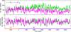Fig. 1 Top panel: solar modulation potential based on GRIP 10Be (magenta) and IntCal13 14C (green) records. Dashed lines show the long-term trend observed in calculated solar modulation potentials. Bottom panel: detrended and standardized solar modulation potential based on polynomial fits of degree 5. The orange and purple colors show dates AD and BC, respectively.

The resulting reconstructions of the solar modulation potential are shown in the top panel of Fig. 1. Even though there is a good agreement between short-term fluctuations (Fig. 1), it is also evident from the figure that there are some discrepancies between the long-term variations of the two reconstructions. The observed long-term differences between the two reconstructions may be caused by long-term changes in the atmospheric transport and deposition of ¹⁰Be and/or undetected changes in carbon cycle (Vonmoos et al. 2006).

To remove the observed long-term trends from the time series, we subtracted the long-term trends (as calculated with polynomial fits of degree 5) from the calculated solar modulation potential values. After removal of the long-term trends from the two time series, we standardized the data using their mean and standard deviation values. The lower panel of Fig. 1 shows the detrended and standardized solar modulation potential reconstructions based on ¹⁰Be and ¹⁴C. Temporal variations in the detrended solar modulation potential reconstructions are in good agreement, implying that short-term variations seen in the reconstructions reflect the solar component within the data.

2.2. Classification of solar cycle events

Temporal variations in the ${\mathrm{\Phi }}_{{\mathrm{10}}^{}\mathrm{Be}}$ and ${\mathrm{\Phi }}_{{\mathrm{14}}^{}\mathrm{C}}$ reconstructions show overlapping events, both as peaks and dips (lower panel of Fig. 1). There are 160 overlapping events in total, whose onset and ending times are determined using a zero-crossing method. The durations of these events range from 5 years (since the records are interpolated) up to ~170 years. To define relevant selection criteria regarding the strength of the peaks and dips, which will be used to identify grand minima and maxima states of the Sun, we construct histograms of the 160 events occurring in both Φ reconstructions between ~1650 AD and 6600 BC during the Holocene epoch. The bin numbers for the histograms are calculated according to the Freedman-Diaconis rule, which aims to minimize the sum of squared errors between the bar heights and the probability distribution of the underlying data (Freedman & Diaconis 1981).

We then tested whether the distributions of the overlapping events are best represented by a normal or a bimodal Gaussian distribution by comparing the Akaike Information Criterion (AIC) and the Bayesian Information Criterion (BIC) values of the two fits (Table 1). The BIC was suggested by Schwarz (1978) as an alternative to the AIC (Akaike 1974) and they are calculated using following equations (Akaike 1974; Schwarz 1978): $\begin{array}{ccc}& & \\ & & \end{array}$where n and k denote the sample size and number of estimated free parameters included in the model, respectively. Gaussian and bimodal Gaussian distributions have 5 and 2 free parameters, respectively. The log-likelihood of the model, represented by the term lnf, reflects the overall fit of the model (Burnham & Anderson 2002) and is calculated as follows (Corsaro et al. 2013): 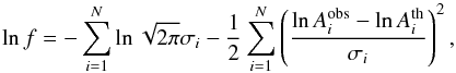$\ln \mathit{f}\mathrm{=}\mathrm{-}\sum _{\mathit{i}\mathrm{=}\mathrm{1}}^{\mathit{N}}\ln \sqrt{\mathrm{2}\mathit{\pi }}{\mathit{\sigma }}_{\mathit{i}}\mathrm{-}\frac{\mathrm{1}}{\mathrm{2}}\sum _{\mathit{i}\mathrm{=}\mathrm{1}}^{\mathit{N}}{\left(\frac{\ln {\mathit{A}}_{\mathit{i}}^{\mathrm{obs}}\mathrm{-}\ln {\mathit{A}}_{\mathit{i}}^{\mathrm{th}}}{{\mathit{\sigma }}_{\mathit{i}}}\right)}^{\mathrm{2}}\mathit{,}$(2)where N is the total number of data points, ${\mathit{A}}_{\mathit{i}}^{\mathrm{obs}}$ and ${\mathit{A}}_{\mathit{i}}^{\mathrm{th}}$ represent observations and the model and σ_i is the uncertainty in observations. Although both criteria are extensions of the maximum likelihood principle and are used to choose the most probable model that best characterizes the data, they are different in some aspects. The BIC is generally used when the main goal is to build a model that describes the distribution of the data, whereas the AIC is used for more predictive aspects (Neath & Cavanaugh 2012). According to Kass & Raftery (1995), if the difference between the BIC values of two distributions (ΔBIC_ab = BIC_a−BIC_b) is less than 2, then the likelihood for model “a” is comparable to that for model “b”, whereas model “a” has considerably less support if the difference is between 3 and 7. For differences larger than 10, model “a” is very unlikely, while model “b” is the most likely model that best represents the data. The same rule is also valid for the AIC values (Burnham & Anderson 2002). The results show that the overlapping events are best represented by bimodal Gaussian fits, since both the AIC and BIC values calculated for the bimodal Gaussian distributions are smaller than those calculated for the normal Gaussian distributions, which are very unlikely according to Kass & Raftery (1995) (Table 1). The bimodal Gaussian fits have mean values of −0.92σ and 1.35σ for the overlapping events observed in the ${\mathrm{\Phi }}_{{\mathrm{10}}^{}\mathrm{Be}}$ reconstruction (left panel of Fig. 2) and −0.67σ and 1.41σ for the overlapping events observed in the ${\mathrm{\Phi }}_{{\mathrm{14}}^{}\mathrm{C}}$ reconstruction (right panel of Fig. 2).

The amplitudes of the events can be characterized by bimodal distributions, implying that the overlapping events through the Holocene epoch show two modes, peaks and dips, with distinct local maxima in the probability density functions (red line in Fig. 2). Based on the local maxima values of the bimodal Gaussian fits, we define threshold values regarding the strengths of the overlapping peaks and dips to identify grand maximum and minimum episodes among these events. Since the distributions of all events in the ${\mathrm{\Phi }}_{{\mathrm{10}}^{}\mathrm{Be}}$ and ${\mathrm{\Phi }}_{{\mathrm{14}}^{}\mathrm{C}}$ reconstructions are not identical and hence yield slightly different local maxima values, we determine the threshold values for maximum and minimum periods for each data set separately.

Fig. 2 Left and right panels show histograms of all events recorded over the Holocene period, which overlap in solar modulation potential reconstructions based on the GRIP 10Be and the IntCal13 14C, respectively. The red line shows the bimodal Gaussian distribution fitted to the data, whereas the texts show the threshold values determined for identifying grand minima and maxima.

We classified all the events according to their amplitudes in three distinct modes (Usoskin et al. 2014): moderate activity level in ${\mathrm{\Phi }}_{{\mathrm{10}}^{}\mathrm{Be}}$ defined as values within −0.92σ and +1.35σ, low activity level for values smaller than −0.92σ, and high-activity level for values higher than +1.35σ. For ${\mathrm{\Phi }}_{{\mathrm{14}}^{}\mathrm{C}}$, moderate activity level is defined as values between −0.67σ and +1.41σ, low activity level for values smaller than −0.67σ and high activity level for values higher than +1.41σ. Within the low- and high-activity groups, we define grand minima and maxima events as intervals lasting more than two sunspot cycles.

Based on the criteria that we define, we identify 32 grand minima and 21 grand maxima periods, which are listed in Tables 2 and 3, respectively. In the ${\mathrm{\Phi }}_{{\mathrm{10}}^{}\mathrm{Be}}$ data, there are two grand minima around 417 AD and −2183 BC (434 AD and −2195 BC in ${\mathrm{\Phi }}_{{\mathrm{14}}^{}\mathrm{C}}$) and three grand maxima around 517 AD, 224 AD, and −6130 BC (521 AD, 200 AD, and −6133 BC in ${\mathrm{\Phi }}_{{\mathrm{14}}^{}\mathrm{C}}$), whose durations show an approximate 50 year difference in comparison to those identified in ${\mathrm{\Phi }}_{{\mathrm{14}}^{}\mathrm{C}}$. The reason for the observed differences in duration may be caused by the different geochemical behavior of the two radionuclides, which can alter the peak shapes.

According to the results obtained using ${\mathrm{\Phi }}_{{\mathrm{10}}^{}\mathrm{Be}}$, the Sun spent ~27% of its time in a grand minimum state and ~16% of its time in a grand maximum state during the last 8250 years. As for ${\mathrm{\Phi }}_{{\mathrm{14}}^{}\mathrm{C}}$, these numbers are ~28% and ~16%, respectively. The total time spent in a minimum state (~27%) we found is higher than that found by Usoskin et al. (2007), whereas our estimate of the time spent in a maximum state lies in between the two estimates obtained by Usoskin et al. (2007) based on two different SSN reconstructions.

Additionally, we have investigated whether the durations of grand minima and grand maxima depend on their amplitude to test if these grand minima and grand maxima events tend to last longer and shorter with respect to the periods characterized by moderate activity levels. Figure 3 clearly suggests that there is a tendency for the grand minima events to last longer than moderate activity periods. For grand maxima, we find an upper limit of 100 years for the durations of the highest amplitudes.

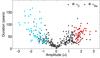Fig. 3 Duration as a function of strength of all events recorded over the Holocene period. Red and blue colors show identified grand maximum and grand minimum periods, respectively. Gray color shows moderate activity periods observed in ${\mathrm{\Phi }}_{{\mathrm{14}}^{}\mathrm{C}}$ and ${\mathrm{\Phi }}_{{\mathrm{10}}^{}\mathrm{Be}}$. Circles and diamonds represents ${\mathrm{\Phi }}_{{\mathrm{14}}^{}\mathrm{C}}$ and ${\mathrm{\Phi }}_{{\mathrm{10}}^{}\mathrm{Be}}$, respectively.

3. Results

3.1. On the origin of grand minima and maxima

Waiting time is defined as the time interval between two subsequent events. The statistical distribution of the waiting times between discrete events has been broadly used in physical sciences to investigate whether the occurrence of these events reflect random or time-dependent, memory-bearing processes (Wheatland 2000; Lepreti et al. 2001; Wheatland 2003). An exponential waiting time distribution indicates that the mechanism causing these events is a Poisson process, which is a memoryless, purely random process, where the occurrence of an event is independent of the preceding event (Usoskin et al. 2007). On the other hand, if the waiting time distribution follows a power-law, the occurrence is dependent on the previous event, implying that the underlying process has a memory (Clauset et al. 2009). A power-law distribution could reflect a number of processes, including self-organized criticality (de Carvalho & Prado 2000; Freeman et al. 2000), a time-dependent Poisson process (Wheatland 2003), or a driving process with a memory (Lepreti et al. 2001; Mega et al. 2003).

Therefore, to investigate the occurrence of the detected grand minimum and maximum activity states of the Sun and durations of these periods, we applied waiting time distribution analyses to the occurrences of detected grand minima and maxima. Waiting times can be considered as intervals between the ending time of an event to the onset of a subsequent event or alternatively the time intervals between subsequent peaks or dips in activity (Wheatland et al. 1998). We applied the latter definition.

Prior to the analyses, we constructed complementary cumulative distribution functions of the occurrences of detected grand minima and maxima, which is defined as the probability that an event “X” with a certain probability distribution will be found at a value more than or equal to “x”. The mathematical formulation is shown below (Clauset et al. 2009; Guerriero 2012): 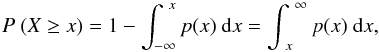$\mathit{P}\mathrm{(}\mathit{X}\mathrm{\ge }\mathit{x}\mathrm{)}\mathrm{=}\mathrm{1}\mathrm{-}{\mathrm{\int }}_{\mathrm{-}\mathrm{\infty }}^{\mathit{x}}\mathit{p}\mathrm{\left(}\mathit{x}\mathrm{\right)}\mathrm{d}\mathit{x}\mathrm{=}{\mathrm{\int }}_{\mathit{x}}^{\mathrm{\infty }}\mathit{p}\mathrm{\left(}\mathit{x}\mathrm{\right)}\mathrm{d}\mathit{x}\mathit{,}$(3)where P denotes the probability. Following this step, we fit a power-law distribution using the algorithm provided by Clauset et al. (2009) and an exponential distribution using the maximum likelihood method (MLM), which takes the real distribution of the data into account. The MLM is robust and accurate for estimation of the parameters of the distributions we consider here (Clauset et al. 2009; Guerriero 2012). The equations used for the power-law (Eq. (4)) and exponential (Eq. (5)) fits are shown below: 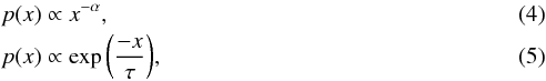$\begin{array}{ccc}& & \mathit{p}\mathrm{\left(}\mathit{x}\mathrm{\right)}\mathrm{\propto }{\mathit{x}}^{\mathrm{-}\mathit{\alpha }}\mathit{,}\\ & & \mathit{p}\mathrm{\left(}\mathit{x}\mathrm{\right)}\mathrm{\propto }\exp \left(\frac{\mathrm{-}\mathit{x}}{\mathit{\tau }}\right)\mathit{,}\end{array}$where p(x) denotes the probability and α and τ indicate the scaling and the survival parameters, respectively (Virkar & Clauset 2014). The resulting fits constructed using the MLM are shown in the top panel of Fig. 4, whereas their scaling and survival parameters are listed in Table 4 together with the BIC and AIC values. The BIC and AIC indicate with high probability that the distribution of waiting times observed for the both ${\mathrm{\Phi }}_{{\mathrm{14}}^{}\mathrm{C}}$ and ${\mathrm{\Phi }}_{{\mathrm{10}}^{}\mathrm{Be}}$ reconstructions are better represented by a power-law fit than an exponential fit, since the differences between the AIC and BIC values for power-law and exponential fits exceed 100. One interesting feature seen in the top left panel of Fig. 4 is that there is an indication of a lumping of waiting times of grand minima periods into three, i.e., one is around 140 years and the other two around 250 and 470 years, respectively. For the top right panel of Fig. 4, which shows waiting times of grand maxima periods, these lumps are seen around 250 and 440 years. The observed tendency for lumping in the top panels of Fig. 4 may indicate that there are different characteristic timescales involved in the system, some of which may potentially be associated with the known solar periodicities of ~150, ~220, and ~400 years (Knudsen et al. 2009). However, Monte Carlo tests show that the observed tendencies for lumping are not statistically significant.

To double-check the results suggested by the BIC and AIC, we generated synthetic data sets using the calculated scaling (α) and survival (τ) parameters of power-law and exponential distributions in Eqs. (4) and (5), respectively, and performed two sample Kolmogorov-Smirnov (KS) tests. For grand minimum and maximum periods, the KS test results suggest that the distributions are better represented by a power-law compared to an exponential fit at the 99% significance level, supporting the results of the BIC and AIC analyses.

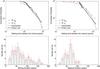Fig. 4 Results of the waiting time distribution analyses. Top panels show the complementary cumulative distribution function for grand minima and grand maxima together with the power-law and exponential fits using MLM. Bottom panels show the distributions of durations of the grand minima and maxima, respectively.

Additionally, we tested whether the distributions of the durations of grand minima and maxima (the bottom panel of Fig. 4) are best represented by Gaussian, lognormal, or bimodal Gaussian distributions. Based on the BIC and AIC values of these fits (Table 5), the durations of grand maxima periods are best represented by a Gaussian distribution with a mean duration of ~65 years, while a lognormal distribution represents the distribution of grand minima durations better with a mean duration of ~70 years, though the significances these findings are low. Usoskin et al. (2007) also suggested that the mean duration for grand minima is 70 years, but claimed that the durations of grand minima show a bimodal Gaussian distribution implying two kinds of minima, i.e., 30 to 90 years, similar to the Maunder minimum, and longer than 110 years, similar to the Spörer minimum.

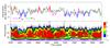Fig. 5 Top panel: temporal change in ${\mathrm{\Phi }}_{{\mathrm{10}}^{}\mathrm{Be}}$ and ${\mathrm{\Phi }}_{{\mathrm{14}}^{}\mathrm{C}}$. Blue and red lines show identified grand minima and maxima, respectively. Bottom panel: local cross-wavelet spectrum of the high-pass filtered ${\mathrm{\Phi }}_{{\mathrm{10}}^{}\mathrm{Be}}$ and ${\mathrm{\Phi }}_{{\mathrm{14}}^{}\mathrm{C}}$ with a cutoff frequency of (1/30) year-1, focusing on identified grand minima periods by our defined criterion. Purple color show the dates BC.

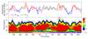Fig. 6 Top panel: temporal change in ${\mathrm{\Phi }}_{{\mathrm{10}}^{}\mathrm{Be}}$ and ${\mathrm{\Phi }}_{{\mathrm{14}}^{}\mathrm{C}}$. Blue and red lines show identified grand minima and maxima, respectively. Bottom panel: local cross-wavelet spectrum of the high-pass filtered ${\mathrm{\Phi }}_{{\mathrm{10}}^{}\mathrm{Be}}$ and ${\mathrm{\Phi }}_{{\mathrm{14}}^{}\mathrm{C}}$ with a cutoff frequency of (1/30) year-1, focusing on identified grand maxima periods by our defined criterion. Orange and purple colors show the dates AD and BC, respectively.

3.2. Magnetic cycle lengths during grand minima and maxima

Previous studies have shown that the cyclic behavior of solar magnetic activity does not cease during grand minimum states (Beer et al. 1998; Owens et al. 2012; McCracken et al. 2013). Even further, based on a ¹⁰Be record from the Dye 3 ice core, Fligge et al. (1999), show that the sunspot cycle lengths during the Spörer Minimum were much longer than 11 years. Hence, we study the cycle-length variation of the Hale cycle (22-year magnetic activity) over the whole Holocene period, more specifically during grand minima and maxima. According to Tobias (1998), we should expect to observe systematic trends in the cycle-length variation over grand minima and maxima.

The bottom panels of Figs. 5 and 6, which focus on the identified grand minima and maxima based on our defined criteria, show the resulting local cross-wavelet power spectra of high-pass filtered ${\mathrm{\Phi }}_{{\mathrm{10}}^{}\mathrm{Be}}$ and ${\mathrm{\Phi }}_{{\mathrm{14}}^{}\mathrm{C}}$ with a cutoff frequency of (1/30) year^-1 together with the solar modulation potential reconstructions based on ¹⁰Be and ¹⁴C, respectively (top panels). The cross-wavelet analyses are based on the algorithm provided by Grinsted et al. (2004). In the figures, we also show minimum and maximum solar activity periods we identified.

An interesting feature observed in the cross-wavelet power spectra is that even though it is difficult to detect the 22-year Hale cycle because of the lack of high-resolution data, it is still possible to follow the temporal behavior of the periods lower than 40 years that are present in the data. When the bottom panels of Figs. 5 and 6 are carefully examined, we observe that the significance of the 22-year Hale cycle during grand minimum and maximum states tends to decrease and increase, respectively, implying that the power of the 22-year Hale cycle under consideration becomes weaker and stronger during grand minima and maxima states. A similar trend can also be observed for the length of the 22-year Hale cycle, which tends to become longer (~30 years) during grand minima states, while it appears to become shorter (~20 years) during grand maxima states.

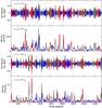Fig. 7 Temporal changes in high-pass filtered ${\mathrm{\Phi }}_{{\mathrm{10}}^{}\mathrm{Be}}$ and ${\mathrm{\Phi }}_{{\mathrm{14}}^{}\mathrm{C}}$ (first and third rows, respectively) with a cutoff frequency of (1/30) year-1. Blue and red lines show identified grand minima and maxima, respectively. The second and forth panels show the moving variance of high-pass filtered ${\mathrm{\Phi }}_{{\mathrm{10}}^{}\mathrm{Be}}$ and ${\mathrm{\Phi }}_{{\mathrm{14}}^{}\mathrm{C}}$. The orange and purple colors show the dates AD and BC, respectively.

A similar feature can also be seen in the high-pass filtered data (Fig. 7). The variance in the data tends to be lower during grand minimum periods in contrast to grand maximum periods, in which the variance tends to be higher. We therefore calculate the moving variance of the two high-pass filtered data sets using a 25-year moving window, which is also shown in Fig. 7. To test the significance of our observations statistically, we carried out KS tests, which are based on the null hypothesis that the two data sets belong to the same continuous distribution. Prior to the KS tests, we separated the moving variance data set into three periods, i.e., grand minima, grand maxima, and periods characterized by intermediate solar activity levels. We also separated the wavelet power spectra of the high-pass filtered data, which is calculated separately for the HP${\mathrm{\Phi }}_{{\mathrm{10}}^{}\mathrm{Be}}$ and the HP${\mathrm{\Phi }}_{{\mathrm{14}}^{}\mathrm{C}}$, into the same three periods. After this step, we average the power obtained between periodicities of 20 and 40 years. The results of the KS tests are shown in Fig. 8. Both the power and the variance observed during grand minimum states are lower at the 99% significance level than those observed during grand maximum states and moderate activity periods. Additionally, the power and variance observed during grand maximum states are higher at the 99% significance level compared to those observed during grand minimum states and during moderate periods. These differences observed for the power and variance are more pronounced in the HP${\mathrm{\Phi }}_{{\mathrm{10}}^{}\mathrm{Be}}$ data than in the HP${\mathrm{\Phi }}_{{\mathrm{14}}^{}\mathrm{C}}$ data. The reason for this difference may be the attenuation effect of the global carbon cycle on the amplitude of the peaks in the ¹⁴C measurements. Combining these findings on the power and variance of the 22-year Hale cycle with its cycle-length variations during grand minima and maxima periods, we suggest that during grand minima and maxima periods the 22-year Hale cycles tend to show weaker and stronger variability and to be longer and shorter compared to moderate activity periods.

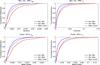Fig. 8 Two sample Kolmogorov-Smirnov test results for HP${\mathrm{\Phi }}_{{\mathrm{10}}^{}\mathrm{Be}}$ and HP${\mathrm{\Phi }}_{{\mathrm{14}}^{}\mathrm{C}}$. Top panels show the results for moving variance, whereas bottom panels show the results for the power seen in HP${\mathrm{\Phi }}_{{\mathrm{10}}^{}\mathrm{Be}}$ and HP${\mathrm{\Phi }}_{{\mathrm{14}}^{}\mathrm{C}}$, respectively. Grand maximum, minimum, and isolated periods are shown with red, blue and gray lines, respectively.

4. Discussion

The combined results from the analyses of ¹⁰Be and ¹⁴C data show that grand minimum and maximum events are likely to represent distinct modes of the solar dynamo resulting from time-dependent, memory-bearing processes, supporting the results found by Usoskin et al. (2014). We also find that there is an apparent upper limit of ~100 years for the duration of grand maxima based on our defined criteria. This can be interpreted as a limit on the capability of the solar dynamo to sustain higher activity levels for longer periods and this number can be directly compared with predictions based on solar dynamos regarding the length of grand maxima. Furthermore, the results of cross-wavelet and KS test analyses suggest that, during grand minima, the power of the 22-year Hale cycle and data variance decrease, while they increase during the grand maxima. These findings could be interpreted based on the fact that at maximum solar activity levels over an 11-year cycle, the poloidal component of the dynamo is at its minimum. As the solar activity level goes into the descending phase, the poloidal component of the dynamo becomes stronger, reaching its maximum at the minimum solar activity of an 11-year cycle. This means that soon after the large-scale dynamo has completed its polarity reversal throughout the whole Sun, the first active regions with opposite polarity compared to the previous 11-year cycle starts to emerge. To sustain the polarity reversals over many cycles, the meridional flow¹ is assumed to be faster during more active cycles, while slower during less active cycles (Wang et al. 2002). This assumption agrees with the observed trend for the more active cycles to have shorter rise times (Schatten & Hedin 1984) and a more rapid progression of sunspots toward the equator (Hathaway et al. 2003). However, during grand minima and maxima, there tends to be subsequently less and more active 11-year cycles compared to times of moderate activity levels. This might alter the time it takes to reverse the polarity throughout the whole Sun due to changes in meridional flow, and hence this period might become shorter and longer compared to intervals characterized by moderate activity levels, respectively. It is also noteworthy that over the last grand maximum, which started in ~1940 and ended with solar cycle 22 (Usoskin 2013), there have been 5 solar cycles, whose durations are below 11 years and only one that lasted almost 11.7 years.

These observational findings that exhibited a long-lasting minimum agree with a recent 3D magnetohydrodynamic anelastic spherical harmonics model. In this model, during a minimum there is an interval covering 20% of the cycles in which the polarity does not reverse and the magnetic energy is substantially reduced (Augustson et al. 2013).

5. Conclusions

In this study, we used two solar modulation potential reconstructions based on IntCal13 ¹⁴C and GRIP ¹⁰Be records to identify the occurrence of grand minima and maxima periods. In order for a low and high activity period to be considered a grand minimum and maximum, it has to occur in both records at the same time with a duration longer than 22 years and with an amplitude below and above a certain threshold value (Sect. 2.2). The results show that the Sun experienced 32 grand minima (~27% of the time) and 21 grand maxima (~16% of the time) episodes during the period from 1650 AD to 6600 BC. A waiting time distribution analysis further shows that the grand minima and maxima periods represent two distinct modes of the solar dynamo and they are likely to be related to time-dependent, memory-bearing processes. This study provides more robust identification of past grand solar minima and maxima periods, which may improve our understanding of the physical processes that cause them, and will allow more systematic and detailed investigations of the possible influences of grand minima and maxima episodes on the Earth’s climate using climate proxy records.

Acknowledgments

Funding for the Stellar Astrophysics Centre is provided by the Danish National Research Foundation (Grant agreement No.: DNRF106). M.F.K., C.K. and J.O. acknowledge support from the Carlsberg Foundation and Villum Foundation. R.S. acknowledge the support from the PiCARD collaboration.

References

All Tables

All Figures

	Fig. 1 Top panel: solar modulation potential based on GRIP 10Be (magenta) and IntCal13 14C (green) records. Dashed lines show the long-term trend observed in calculated solar modulation potentials. Bottom panel: detrended and standardized solar modulation potential based on polynomial fits of degree 5. The orange and purple colors show dates AD and BC, respectively.
In the text

	Fig. 2 Left and right panels show histograms of all events recorded over the Holocene period, which overlap in solar modulation potential reconstructions based on the GRIP 10Be and the IntCal13 14C, respectively. The red line shows the bimodal Gaussian distribution fitted to the data, whereas the texts show the threshold values determined for identifying grand minima and maxima.
In the text

Fig. 3 Duration as a function of strength of all events recorded over the Holocene period. Red and blue colors show identified grand maximum and grand minimum periods, respectively. Gray color shows moderate activity periods observed in ${\mathrm{\Phi }}_{{\mathrm{14}}^{}\mathrm{C}}$ and ${\mathrm{\Phi }}_{{\mathrm{10}}^{}\mathrm{Be}}$. Circles and diamonds represents ${\mathrm{\Phi }}_{{\mathrm{14}}^{}\mathrm{C}}$ and ${\mathrm{\Phi }}_{{\mathrm{10}}^{}\mathrm{Be}}$, respectively.

In the text

	Fig. 4 Results of the waiting time distribution analyses. Top panels show the complementary cumulative distribution function for grand minima and grand maxima together with the power-law and exponential fits using MLM. Bottom panels show the distributions of durations of the grand minima and maxima, respectively.
In the text

Fig. 5 Top panel: temporal change in ${\mathrm{\Phi }}_{{\mathrm{10}}^{}\mathrm{Be}}$ and ${\mathrm{\Phi }}_{{\mathrm{14}}^{}\mathrm{C}}$. Blue and red lines show identified grand minima and maxima, respectively. Bottom panel: local cross-wavelet spectrum of the high-pass filtered ${\mathrm{\Phi }}_{{\mathrm{10}}^{}\mathrm{Be}}$ and ${\mathrm{\Phi }}_{{\mathrm{14}}^{}\mathrm{C}}$ with a cutoff frequency of (1/30) year-1, focusing on identified grand minima periods by our defined criterion. Purple color show the dates BC.

In the text

Fig. 6 Top panel: temporal change in ${\mathrm{\Phi }}_{{\mathrm{10}}^{}\mathrm{Be}}$ and ${\mathrm{\Phi }}_{{\mathrm{14}}^{}\mathrm{C}}$. Blue and red lines show identified grand minima and maxima, respectively. Bottom panel: local cross-wavelet spectrum of the high-pass filtered ${\mathrm{\Phi }}_{{\mathrm{10}}^{}\mathrm{Be}}$ and ${\mathrm{\Phi }}_{{\mathrm{14}}^{}\mathrm{C}}$ with a cutoff frequency of (1/30) year-1, focusing on identified grand maxima periods by our defined criterion. Orange and purple colors show the dates AD and BC, respectively.

In the text

Fig. 7 Temporal changes in high-pass filtered ${\mathrm{\Phi }}_{{\mathrm{10}}^{}\mathrm{Be}}$ and ${\mathrm{\Phi }}_{{\mathrm{14}}^{}\mathrm{C}}$ (first and third rows, respectively) with a cutoff frequency of (1/30) year-1. Blue and red lines show identified grand minima and maxima, respectively. The second and forth panels show the moving variance of high-pass filtered ${\mathrm{\Phi }}_{{\mathrm{10}}^{}\mathrm{Be}}$ and ${\mathrm{\Phi }}_{{\mathrm{14}}^{}\mathrm{C}}$. The orange and purple colors show the dates AD and BC, respectively.

In the text

Fig. 8 Two sample Kolmogorov-Smirnov test results for HP${\mathrm{\Phi }}_{{\mathrm{10}}^{}\mathrm{Be}}$ and HP${\mathrm{\Phi }}_{{\mathrm{14}}^{}\mathrm{C}}$. Top panels show the results for moving variance, whereas bottom panels show the results for the power seen in HP${\mathrm{\Phi }}_{{\mathrm{10}}^{}\mathrm{Be}}$ and HP${\mathrm{\Phi }}_{{\mathrm{14}}^{}\mathrm{C}}$, respectively. Grand maximum, minimum, and isolated periods are shown with red, blue and gray lines, respectively.

In the text

References

- Abreu, J. A., Beer, J., Steinhilber, F., Tobias, S. M., & Weiss, N. O. 2008, Geophys. Res. Lett., 35, L20109 [NASA ADS] [CrossRef] [Google Scholar]
- Akaike, H. 1974, IEEE Transactions on Automatic Control, AC-19, 6 [Google Scholar]
- Aldahan, A., Hedfors, J., Possnert, G., et al. 2008, Geophys. Res. Lett., 35, 21812 [NASA ADS] [CrossRef] [Google Scholar]
- Augustson, K., Brun, A. S., Miesch, M. S., & Toomre, J. 2013, ApJL, submitted, ArXiv e-prints [arXiv:1310.8417] [Google Scholar]
- Baliunas, S. L., Donahue, R. A., Soon, W. H., et al. 1995, ApJ, 438, 269 [NASA ADS] [CrossRef] [Google Scholar]
- Bard, E., Raisbeck, G. M., Yiou, F., & Jouzel, J. 1997, Earth Planet. Sci. Lett., 150, 453 [NASA ADS] [CrossRef] [Google Scholar]
- Beer, J., Tobias, S., & Weiss, N. 1998, Sol. Phys., 181, 237 [Google Scholar]
- Berggren, A.-M., Beer, J., Possnert, G., et al. 2009, Geophys. Res. Lett., 36, 11801 [Google Scholar]
- Brandenburg, A., Krause, F., Meinel, R., Moss, D., & Tuominen, I. 1989, A&A, 213, 411 [NASA ADS] [Google Scholar]
- Burnham, K. P., & D. R. Anderson, 2002, Model Selection and Multimodel Inference: a practical information-theoretic approach, 2nd edn. (New York: Springer-Verlag) [Google Scholar]
- Clauset, A., Rohil la Shalizi, C., & Newman, M. E. J. 2009, Soc. Industrial Appl. Math. Rev., 51, 4 [Google Scholar]
- Corsaro, E., Fröhlich, H.-E., Bonanno, A., et al. 2013, MNRAS, 430, 2313 [NASA ADS] [CrossRef] [Google Scholar]
- de Carvalho, J. X., & Prado, C. P. C. 2000, Phys. Rev. Lett., 84, 4006 [NASA ADS] [CrossRef] [PubMed] [Google Scholar]
- DeRosa, M. L., Brun, A. S., & Hoeksema, J. T. 2012, ApJ, 757, 96 [Google Scholar]
- Dikpati, M., Gilman, P. A., de Toma, G., & Ulrich, R. K. 2010, Geophys. Res. Lett., 37, 14107 [NASA ADS] [Google Scholar]
- Dunai, T. J. 2010, in Cosmogenic Nuclides: Principles, Concepts and Applications in the Earth Surface Sciences (Cambridge: Cambridge University Press), 2 [Google Scholar]
- Field, C. V., Schmidt, G. A., Koch, D., & Salyk, C. 2006, J. Geophys. Res., 111, 15107 [Google Scholar]
- Fligge, M., Solanki, S. K., & Beer, J. 1999, A&A, 346, 313 [NASA ADS] [Google Scholar]
- Freedman, D., & Diaconis, P. 1981, Z. für Wahrscheinlichkeitstheorie Verwandte Gebiete, 57, 453 [Google Scholar]
- Freeman, M. P., Watkins, N. W., & Riley, D. J. 2000, Phys. Rev. E, 62, 8794 [Google Scholar]
- Grinsted, A., Moore, J. C., & Jevrejeva, S. 2004, Nonlinear Processes Geophys., 11, 561 [NASA ADS] [CrossRef] [Google Scholar]
- Guerriero, V. 2012, J. Mod. Math. Frontier, 1, 21 [Google Scholar]
- Hathaway, D. H., Nandy, D., Wilson, R. M., & Reichmann, E. J. 2003, ApJ, 589, 665 [NASA ADS] [CrossRef] [Google Scholar]
- Kass, R., & Raftery, A. 1995, J. Am. Stat. Assoc., 90, 773 [Google Scholar]
- Knudsen, M. F., Riisager, P., Jacobsen, B. H., et al. 2009, Geophys. Res. Lett., 36, 16701 [Google Scholar]
- Koch, D., & Rind, D. 1998, J. Geophys. Res., 103, 3907 [Google Scholar]
- Lepreti, F., Carbone, V., & Veltri, P. 2001, ApJ, 555, L133 [Google Scholar]
- Lockwood, M. 2013, Liv. Rev. Sol. Phys., 10, 4 [Google Scholar]
- Masarik, J., & Beer, J. 1999, J. Geophys. Res., 104, 12099 [NASA ADS] [CrossRef] [Google Scholar]
- McCracken, K., Beer, J., Steinhilber, F., & Abreu, J. 2013, Space Sci. Rev., 176, 59 [NASA ADS] [CrossRef] [Google Scholar]
- Mega, M. S., Allegrini, P., Grigolini, P., et al. 2003, Phys. Rev. Lett., 90, 188501 [NASA ADS] [CrossRef] [PubMed] [Google Scholar]
- Moss, D., Sokoloff, D., Usoskin, I., & Tutubalin, V. 2008, Sol. Phys., 250, 221 [NASA ADS] [CrossRef] [Google Scholar]
- Neath, A. A., & Cavanaugh, J. E. 2012, WIREs Comput. Stat., 4, 199 [CrossRef] [Google Scholar]
- Owens, M. J., Usoskin, I., & Lockwood, M. 2012, Geophys. Res. Lett., 39, 19102 [Google Scholar]
- Parker, E. N. 1955a, ApJ, 122, 293 [NASA ADS] [CrossRef] [Google Scholar]
- Parker, E. N. 1955b, ApJ, 121, 491 [NASA ADS] [CrossRef] [Google Scholar]
- Raisbeck, G. M., Yiou, F., Fruneau, M., et al. 1981, Nature, 292, 825 [NASA ADS] [CrossRef] [Google Scholar]
- Reimer, P. J., et al. 2013, Radiocarbon, 55, 1869 [CrossRef] [Google Scholar]
- Roth, R., & Joos, F. 2013, Climate of the Past, 9, 1879 [Google Scholar]
- Schatten, K. H., & Hedin, A. E. 1984, Geophys. Res. Lett., 11, 873 [NASA ADS] [CrossRef] [Google Scholar]
- Schwarz, G. 1978, The Annals of Statistics, 6, 461 [Google Scholar]
- Stuiver, M. 1980, Nature, 286, 868 [NASA ADS] [CrossRef] [Google Scholar]
- Stuiver, M., & Braziunas, T. F. 1989, Nature, 338, 405 [NASA ADS] [CrossRef] [Google Scholar]
- Suess, H. E. 1955, Science, 122, 415 [NASA ADS] [CrossRef] [Google Scholar]
- Tobias, S. M. 1996, A&A, 307, L21 [NASA ADS] [Google Scholar]
- Tobias, S. M. 1997, A&A, 322, 1007 [NASA ADS] [Google Scholar]
- Tobias, S. M. 1998, MNRAS, 296, 653 [NASA ADS] [CrossRef] [Google Scholar]
- Usoskin, I. G. 2013, Liv. Rev. Sol. Phys., 10, 1 [Google Scholar]
- Usoskin, I. G., Solanki, S. K., & Kovaltsov, G. A. 2007, A&A, 471, 301 [NASA ADS] [CrossRef] [EDP Sciences] [Google Scholar]
- Usoskin, I. G., Hulot, G., Gallet, Y., et al. 2014, A&A, 562, L10 [NASA ADS] [CrossRef] [EDP Sciences] [Google Scholar]
- Virkar, Y., & Clauset, A. 2014, Ann. Appl. Statist., 8, 89 [Google Scholar]
- Vonmoos, M., Beer, J., & Muscheler, R. 2006, J. Geophys. Res., 111, 10105 [NASA ADS] [CrossRef] [Google Scholar]
- Voss, H., Kurths, J., & Schwarz, U. 1996, J. Geophys. Res., 101, 15637 [NASA ADS] [CrossRef] [Google Scholar]
- Wang, Y.-M., Lean, J., & Sheeley, Jr. N. R. 2002, ApJ, 577, L53 [Google Scholar]
- Wheatland, M. S. 2000, ApJ, 536, L109 [NASA ADS] [CrossRef] [PubMed] [Google Scholar]
- Wheatland, M. S. 2003, Sol. Phys., 214, 361 [NASA ADS] [CrossRef] [Google Scholar]
- Wheatland, M. S., Sturrock, P. A., & McTiernan, J. M. 1998, ApJ, 509, 448 [NASA ADS] [CrossRef] [Google Scholar]
All Tables
Bayesian (BIC) and Akaike (AIC) information criterion values for Gaussian and bimodal Gaussian fits.
List of grand minima found in solar modulation potential data based on our criteria.
List of the grand maxima found in solar modulation potential data based on our criteria.
Scaling and survival parameters found for grand minima, maxima, and duration of these periods using maximum likelihood method for power-law and exponential fits together with the Bayesian (BIC) and Akaike (AIC) information criterion values.
Bayesian (BIC) and Akaike (AIC) information criterion values for Gaussian, lognormal and bimodal Gaussian fits to the durations of grand maxima and grand minima.