| Issue |
A&A
Volume 577, May 2015
|
|
|---|---|---|
| Article Number | A63 | |
| Number of page(s) | 14 | |
| Section | Astrophysical processes | |
| DOI | https://doi.org/10.1051/0004-6361/201423402 | |
| Published online | 05 May 2015 | |
A possible cyclotron resonance scattering feature near 0.7 keV in X1822-371
1
Dipartimento di Fisica e ChimicaUniversità di Palermo,
via Archirafi 36,
90123
Palermo,
Italy
e-mail:
This email address is being protected from spambots. You need JavaScript enabled to view it.
2
Dipartimento di Fisica, Università degli Studi di
Cagliari, SP Monserrato-Sestu, KM
0.7, 09042
Monserrato,
Italy
3
ISDC, Department of Astronomy, Université de Genève,
chemin d’Écogia, 16,
1290
Versoix,
Switzerland
4
Istituto Nazionale di Astrofisica, IASF Palermo, via U. La Malfa
153, 90146
Palermo,
Italy
Received: 11 January 2014
Accepted: 3 March 2015
Abstract
Context. The source X1822-371 is a low-mass X-ray binary system (LMXB) viewed at a high inclination angle. It hosts a neutron star with a spin period of ~0.59 s, and recently, the spin period derivative was estimated to be (−2.43 ± 0.05) × 10-12 s/s.
Aims. Our aim is to address the origin of the large residuals below 0.8 keV previously observed in the XMM/EPIC-pn spectrum of X1822-371.
Methods. We analyse all available X-ray observations of X1822-371 made with XMM-Newton, Chandra, Suzaku and INTEGRAL satellites. The observations were not simultaneous. The Suzaku and INTEGRAL broad band energy coverage allows us to constrain the spectral shape of the continuum emission well. We use the model already proposed for this source, consisting of a Comptonised component absorbed by interstellar matter and partially absorbed by local neutral matter, and we added a Gaussian feature in absorption at ~0.7 keV. This addition significantly improves the fit and flattens the residuals between 0.6 and 0.8 keV.
Results. We interpret the Gaussian feature in absorption as a cyclotron resonant scattering feature (CRSF) produced close to the neutron star surface and derive the magnetic field strength at the surface of the neutron star, (8.8 ± 0.3) × 1010 G for a radius of 10 km. We derive the pulse period in the EPIC-pn data to be 0.5928850(6) s and estimate that the spin period derivative of X1822-371 is (−2.55 ± 0.03) × 10-12 s/s using all available pulse period measurements. Assuming that the intrinsic luminosity of X1822-371 is at the Eddington limit and using the values of spin period and spin period derivative of the source, we constrain the neutron star and companion star masses. We find the neutron star and the companion star masses to be 1.69 ± 0.13 M⊙ and 0.46 ± 0.02 M⊙, respectively, for a neutron star radius of 10 km.
Conclusions. In a self-consistent scenario in which X1822-371 is spinning-up and accretes at the Eddington limit, we estimate that the magnetic field of the neutron star is (8.8 ± 0.3) × 1010 G for a neutron star radius of 10 km. If our interpretation is correct, the Gaussian absorption feature near 0.7 keV is the very first detection of a CRSF below 1 keV in a LMXB.
Key words: X-rays: binaries / stars: magnetic field / accretion, accretion disks / X-rays: general / stars: individual: X1822-371
© ESO, 2015
1. Introduction
Neutron stars (NS) are thought to be born with magnetic fields (B-fields) above ~1012 G. Direct measurements of the strength of these fields come from the detection of cyclotron resonant scattering features (CRSFs). In accreting NS, X-ray pulsations and CRSFs are common in systems containing a young high-mass companion (HMXBs), with typical strengths of the NS B-field between 1012–1013 G, whereas in binary systems containing a low-mass companion (LMXBs) pulsations are detected only in a small fraction of systems, and no CRSF has been detected to date. The most likely explanation is that in such systems, the NS B-field is sufficiently decayed in the course of its evolution to a value that, at accretion rates corresponding to 1035–1038 erg s-1, the corresponding magnetospheric radius becomes smaller than the NS radius.
In LMXBs when pulsations are detected, the inferred NS B-fields are of the order of 108–109 G, which is about three orders of magnitude less than the typical values for HMXBs. Intermediate values of the NS B-field, between these two ranges, are uncommonly observed, most probably for evolutionary reasons. However, some notable exceptions exist, such as (i) the 11 Hz pulsar IGR J17480-2446 (Papitto et al. 2011), whose NS B-field was estimated in the range 2 × 10⁸–2.4 × 10¹⁰ G; (ii) the 2.1 Hz X-ray pulsar GRO J1744-28, with an estimated NS B-field of ~2.4 × 10¹¹ G (Cui 1997); and, finally; (iii) the 1.7 Hz X1822-371 (Jonker & van der Klis 2001).
Despite the small sample that it belongs to, the peculiarity of X1822-371 still stands out. Analysing the RXTE data of X1822-371, Jonker & van der Klis (2001) detected for the first time a coherent pulsation at 0.593 s associated with the NS spin period and inferred a spin period derivative of (−2.85 ± 0.04) × 10-12 s s-1. Analysing RXTE data from 51 976 to 52 883 MJD, Jain et al. (2010) constrained the spin period derivative better, finding (−2.481 ± 0.004) × 10-12 s s-1. The ephemeris of X1822-371 has recently been updated by Iaria et al. (2011), who estimated an orbital period of 5.5706124(7) h and an orbital period derivative of (1.51 ± 0.08) × 10-10 s s-1 when analysing X-ray data spanning 30 years. A similar sample of data was analysed by Burderi et al. (2010) who obtained an orbital period derivative of (1.50 ± 0.07) × 10-10 s s-1. In an independent paper, Jain et al. (2010) obtained an orbital period derivative of (1.3 ± 0.3) × 10-10 s s-1 from X-ray data and, studying the optical and UV data of X1822-371, Bayless et al. (2010) derived the new optical ephemeris for the source finding an orbital period derivative of (2.1 ± 0.2) × 10-10 s s-1.
Burderi et al. (2010) show that the orbital-period derivative is three orders of magnitude larger than what is expected from conservative mass transfer driven by magnetic braking and/or gravitational radiation. They conclude that the mass transfer rate from the companion star is between 3.5 and 7.5 times the Eddington limit (~1.1 × 10¹⁸ g s-1 for a NS mass of 1.4 M⊙ and NS radius of 10 km), suggesting that the mass transfer has to be highly non-conservative, with the NS accreting at the Eddington limit and the rest of the transferred mass expelled from the system by the radiation pressure. Bayless et al. (2010) show that the accretion rate onto the NS should be ~6.4 × 10⁻⁸M⊙ yr-1 in a conservative mass transfer scenario, again suggesting a highly non-conservative mass transfer.
The large orbital period derivative is a clear clue that the intrinsic luminosity of X1822-371 is at the Eddington limit, which is almost two orders of magnitude higher than the observed luminosity (i.e. ~1036 erg s-1, see e.g. Hellier & Mason 1989; Heinz & Nowak 2001; Parmar et al. 2000; Iaria et al. 2001). This is also supported by the ratio LX/Lopt of X1822-371. Hellier & Mason (1989) showed that the ratio LX/Lopt for X1822-371 is ~20, a factor 50 smaller than the typical value of 1000 for the other LMXBs. This suggests that the intrinsic X-ray luminosity is underestimated by at least a factor of 50. Finally, Jonker & van der Klis (2001) show that for a luminosity of 1036 erg s-1, the NS B-field strength assumes an unlikely value of 8 × 10¹⁶ G, while for a luminosity of the source of ~1038 erg s-1, it assumes a more conceivable value of 8 × 10¹⁰ G.
Recently when analysing an XMM-Newton observation of X1822-371 and using RGS and EPIC-pn data, Iaria et al. (2013) fitted the X-ray spectrum of this source to a model consisting of a Comptonised component CompTT1 absorbed by interstellar neutral matter and partially absorbed by local neutral matter. The authors took the Thomson scattering of the local neutral matter into account by adding the cabs1 component and imposed that the equivalent hydrogen column density of the cabs component is the same as the local neutral matter. The adopted model is similar to the one previously used by Iaria et al. (2001) to fit the averaged BeppoSAX spectrum of X1822-371. Iaria et al. (2013) suggest that the Comptonised component is produced in the inner regions of the system, which are not directly observable. The observed flux is only 1% of the total intrinsic luminosity, the fraction scattered along the line of sight by an extended optically thin corona with an optical depth τ ≃ 0.01. This scenario explains why the observed luminosity of the source is ~1036 erg s-1, while the orbital period derivative suggests an intrinsic luminosity of X1822-371 at the Eddington limit. Furthermore, Iaria et al. (2013) found that large residuals are present in the EPIC-pn spectrum below 0.9 keV and fitted those residuals by adding a black-body component with a temperature of 0.06 keV, although they suggest that further investigations were needed to understand the physical origin of this component.
Recently, Sasano et al. (2014) have analysed a Suzaku observation of X1822-371 in the 1–45 keV energy range. The authors detect the NS pulsation in the HXD/PIN instrument at 0.5924337(1) s and inferred a spin period derivative of (−2.43 ± 0.05) × 10-12 s/s. Sasano et al. (2014) also suggest the presence of a CRSF at 33 keV and inferred from this value a NS B-field of ~2.8 × 10¹² G and a luminosity of the source of ~3 × 1037 erg s-1.
In this work we determine the NS spin period of X1822-371 during the XMM-Newton observation and derive a new estimation of the spin period derivative, also taking all the measurements of the spin period reported in literature into account, including our derived value. We analyse the combined spectra of X1822-371 obtained with XMM-Newton, Chandra (the same data sets as analysed by Iaria et al. 2013), Suzaku (the same data set as analysed by Sasano et al. 2014), and INTEGRAL. We show the presence of large residuals close to 0.7 keV, while we do not find evidence of a cyclotron feature at 33 keV, unlike what has been suggested by Sasano et al. (2014). Moreover, we show that a CRSF at 33 keV would not be consistent with the evidence that the NS in X1822-371 is spinning up. Fitting the residuals near 0.7 keV with a CRSF centered at 0.72 keV, we determine a NS B-field (surface) strength between 7.8 × 10¹⁰ and 9.3 × 10¹⁰ G for a NS radius ranging between 9.5 and 11.5 km.
2. Observations
2.1. The Suzaku observation
The X-ray satellite Suzaku observed X1822-371 on 2006 October 2 with an elapsed time of 88 ks. Both the X-ray Imaging Spectrometers (0.2–12 keV, XISs; Koyama et al. 2007) and the Hard X-ray Detector (10–600 keV, HXD; Takahashi et al. 2007) instruments were used during these observations. There are four XIS detectors, numbered as 0 to 3. XIS0, XIS2, and XIS3 all use front-illuminated CCDs and have very similar responses, while XIS1 uses a back-illuminated CCD. The HXD instrument includes both positive intrinsic negative (PIN) diodes working between 10 and 70 keV and the gadolinium silicate (GSO) scintillators working between 30–600 keV. Both the PIN and GSO are collimated (non-imaging) instruments. During the observation, XIS0 and XIS1 worked in 1/4 Window option, while XIS2 and XIS3 worked in full window. The effective exposure time of each XIS CCD is nearly 38 ks, and the HXD/PIN exposure time is nearly 31 ks.
We reprocessed the data using the aepipeline tool provided by Suzaku FTOOLS version 202 and applying the latest calibration available as of 2013 November. We then applied the publicly available tool aeattcor.sl3 by John E. Davis to obtain a new attitude file for each observation. This tool corrects the effects of thermal flexing of the Suzaku spacecraft and obtains a more accurate estimate of the spacecraft attitude. For our observation, the above attitude correction produces sharper point-spread-function (PSF) images. With the new attitude file, we updated the XIS event files using the FTOOLS xiscoord program. We estimated the pile-up fractions using the publicly available tool pileup_estimate.sl4 by Michael A. Nowak. The pile-up fraction refers to the ratio of events lost via grade or energy migration to the events expected in the absence of pile-up. The unfiltered pile-up fractions integrated over a circular region centred on the brightest pixel of the CCD and with a radius of 105″ are 4.6%, 3.9%, 10.4%, and 9.9% for XIS0, XIS1, XIS2, and XIS3, respectively. The large pile-up fraction in XIS2 and XIS3 is due to the two CCDs working in full window during the observation. To mitigate the pile-up effects in the spectra extracted from XIS2 and XIS3, we used annular regions, while we adopted circular regions with a radius of 105″ to extract the spectra from XIS0 and XIS1. Adopting annulus regions with inner and outer radii of 28″ and 105″, respectively, the pile-up fractions are 4.8% for XIS2 and 4.6% for XIS3. The background spectra were extracted using the same regions as were adopted to extract the source spectra and centred where the influence of the source photons is weak (or absent) in the CCDs. The response files of the XIS for each observation were generated using the xisrmfgen Suzaku tool, and the corresponding ancillary files were extracted using the xisarfgen Suzaku tool, suitable for a point-like source. Because the responses of XIS0, XIS2, and XIS3 are on the whole very similar, we combined their spectra and responses using the script addascaspec. The XIS spectra were rebinned to have 1024 energy channels.
We also extracted the PIN spectra using the Suzaku tool hxdpinxbpi. The non X-ray and cosmic X-ray backgrounds were taken into account. The non X-ray background (NXB) was calculated from the background event files distributed by the HXD team. The cosmic X-ray background (CXB) is from the model by Boldt (1987). The response files provided by the HXD team were used. The GSO data were not used, considering the low signal-to-noise ratio above 40 keV.
2.2. The XMM-Newton observation
The region of the sky containing X1822-371 was observed by XMM-Newton between 2001 March 07 13:12:48 UT and March 08 03:32:53 UT (Obs. ID. 0111230101) for a duration of 53.8 ks. The European Photon Imaging Camera (EPIC) on-board XMM-Newton consists of three co-aligned high-throughput X-ray telescopes. Imaging charge-coupled-device (CCD) detectors were placed in the focus of each telescope. Two of the CCD detectors are Metal Oxide Semi-conductor (MOS) CCD arrays (see Turner et al. 2001), while the third camera uses pn CCDs (hereafter EPIC-pn, see Strüder et al. 2001). Behind the two telescopes that have the MOS cameras in the focus, about half of the X-ray light is utilised by the reflection grating spectrometers (RGSs). Each RGS consists of an array of reflection gratings that diffracts the X-rays to an array of dedicated CCD detectors (see Brinkman et al. 1998; den Herder et al. 2001).
During the observation, MOS1 and MOS2 camera were operated in fast uncompressed mode and small window mode, respectively. The EPIC-pn camera was operated in timing mode with a medium filter during the observation. The faster CCD readout results in a much higher count rate capability of 800 cts/s before charge pile-up become a serious problem for point-like sources. The EPIC-pn count rate of the source was around 55 cts/s, thereby avoiding telemetry and pile-up problems.
Although the RGS and EPIC-pn data products were extracted and analysed by Iaria et al. (2013), we extracted the data products of the RGS and EPIC-pn camera again using the very recent science analysis software (SAS) version 13.5.0 and the calibration files available on 2013 Dec. 17. We used the SAS tools rgsproc, emproc, and epproc to obtain the RGS, MOS, and EPIC-pn data products.
Since the EPIC-pn was operated in timing mode during the observation, we extracted the EPIC-pn image of RAWX vs. PI to select appropriately the source and background region. The source spectrum is selected from a box region centred on RAWX = 38 with a width of 18 columns. The background spectrum was selected from a box region centred on RAWX = 5 with a width of two columns. We extracted only single and double events (patterns 0 to 4) for the source and background spectra and applied the SAS tool backscale to calculate the different areas of the source and background regions.
We extracted the MOS1 source spectrum, adopting a box region centred on RAWX = 317 having a width of 50 pixels. The MOS1 background spectrum is extracted from a source-free region selected in one of the outer CCDs that collect photons in imaging mode during the observation. We extracted the MOS1 spectrum and the corresponding redistribution matrix and ancillary files using the standard recipe5. We also extracted the source+background light curve, observing that the average count rate during the observation is 15 c/s. The MOS2 source spectrum was extracted from a circular region centred on the pixel showing the largest number of photons; the radius of the region is 640 pixels. A circle with radius of 640 pixels was placed in a source-free region to extract the background spectrum. We extracted the MOS2 spectrum and the corresponding redistribution matrix and ancillary files using the standard recipe6. We also extracted the background-subtracted light curve using the SAS tool Epiclccorr, and the average count rate is 15 c/s. Since the count-rate limit for avoiding pile-up for the MOS cameras is 100 c/s and 5 c/s for a point-like source in timing uncompressed and small window modes7, respectively, we expect that the pile-up effects are present in the MOS2 spectrum. The RGS1, RGS2, MOS1, MOS2, and EPIC-pn spectra have an exposure time of 53, 51, 51, 51, and 51 ks, respectively.
2.3. The Chandra observations
The Chandra satellite observed X1822-371 from 2008 May 20 22:53:00 to 2008 May 21 17:06:51 UT (Obs. ID. 9076) and from 2008 May 23 13:20:56 to 2008 May 24 12:41:54 UT (Obs. ID. 9858) using the HETGS for total observation times of 66 and 84 ks, respectively. Both observations were performed in timed faint mode. The two Chandra observations had already been analysed by Iaria et al. (2013). In this work we only used the first-order MEG spectrum (see Iaria et al. 2013, for details on the data extraction) because the first-order HEG spectrum has a much lower effective area with respect to MEG below 1 keV, and its analysis is not useful for investigating the presence of features in the spectrum of X1822-371 at those energies. The first-order MEG spectrum has a total exposure time of 142 ks.
2.4. The INTEGRAL observations
The INTErnational Gamma-Ray Astrophysics Laboratory (INTEGRAL Winkler et al. 2003) has repeatedly observed the X1822-371 region. We searched the whole IBIS (Ubertini et al. 2003) and JEM-X (Lund et al. 2003) public catalogues, selecting only pointings (science windows, SCW) with sources within six degrees of the centre of the field of view and with exposures longer than 500 s to reduce the calibration uncertainties of the IBIS/ISGRI (Lebrun et al. 2003) spectral response. The available IBIS data set covers the period starting from 2003 March 21 until 2013 March 21 for a total usable on-source time of 1271 ks and an effective dead-time corrected exposure of 874 ks. Because of the smaller field of view, the total exposure of JEM-X1 (camera 1) is 330 ks, while the dead-time-corrected exposure is 283 ks. The INTEGRAL data analysis uses standard procedures within the offline science analysis software (OSA10.0) distributed by the ISDC (Courvoisier et al. 2003). In the catalogue used for the extraction of the IBIS spectra, we have included all the sources significantly detected in the total image obtained by mosaicking the individual pointings. We exploited a custom spectral binning optimised in the energy range 20–100 keV, and in the detection of spectral features around 30 keV, weighted the time-evolving response function according to the available data and excluded the data below 21 keV due to the evolving detector’s low threshold. For JEM-X, we adopted the standard 16 bins spectrum provided by the analysis software and excluded the data below 5 keV and above 22 keV, which are affected by calibration uncertainties8.
3. Search for the spin period in the XMM data
We used the EPIC-pn events to search for the spin period. We applied the barycentric correction with respect to the source coordinates, given by Iaria et al. (2011), using the SAS tool barycen; subsequently, we corrected the data for the orbital motion of the binary system using the recent X-ray ephemeris of X1822-371 derived by (Iaria et al. 2011; see Eq. (2) in that work) and the asini value of 1.006 lt-s (see Table 1 in Jonker & van der Klis 2001). We selected the EPIC-pn events in the 2–5.4 keV energy range and explored the period window between 0.592384 and 0.593384 s using the FTOOL efsearch in the XRONOS package. We adopted eight phase bins per period (a bin time close to 0.074 s) for the trial folded light curves and a resolution of the period search of 1 × 10⁻⁶ s. We observed a χ2 peak of 41.89 at 0.592884 s, as shown in Fig. 1. We fitted the peak with a Gaussian function, assumed the centroid of the Gaussian as the best estimation of the spin period, and associated the error derived from the best fit. We find that the spin period during the XMM observation is 0.5928850(6) s, and the associated error is at the 68% confidence level.
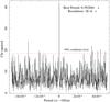 |
Fig. 1 Folding search for periodicities in the 2–5.4 keV EPIC-pn light curve. We adopt 8 phase bins per period for the trial-folded light curves and a resolution of period search of 1 × 10⁻⁶ s. The peak of χ2 is detected at 0.592884 s. The horizontal dashed line indicate the χ2 value of 18.47 at which we have the 99% confidence level for a single trial. |
Considering that we have seven degrees of freedom, the probability of obtaining a χ2 value greater than or equal to 41.89 by chance is 5.47 × 10⁻⁷ for a single trial. In our search we adopted 103 trials (we span 10-3 s with a resolution of the period search of 1 × 10⁻⁶), consequently we expect a number of ≃5.5 × 10⁻⁴ periods with a χ2-value greater than or equal to 41.89. This implies that our detection is significant at the 99.945% confidence level.
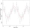 |
Fig. 2 EPIC-pn folded light curves of X1822-371 using the folding period 0.5928850(6) s. The folded light curve is obtained using 16 phase bins per period. |
Then, we folded the 2–5.4 keV EPIC-pn light curve using the spin period of 0.5928850(6) s and adopting 16 phase bins per period. We used the arbitrary value of 51 975.85 MJD as epoch of reference. The folded light curve is almost sinusoidal (see Fig. 2). Fitting the folded light curve with a constant plus a sinusoidal function with period fixed at one, we obtain a χ2(d.o.f.) of 13.9(13). Since the constant is 23.92(2) c/s, the background count rate is close to 1.3 c/s and the amplitude of the sinusoidal function 0.17(3) c/s, we estimate that the pulse fraction is 0.75 ± 0.13% compatible within 3σ to the value of 0.25 ± 0.06% reported by Jonker & van der Klis (2001) using RXTE/PCA data in the same energy band.
Times and corresponding.
We report in Table 1 the 13 values of the spin period of X1822-371 and the corresponding errors previously estimated, together with the value found in the present work. The corresponding times are the mean values between the start and stop time of the observations in which the spin period was detected, the associated errors are one half of the duration of the corresponding observation. After deriving the geometric mean of the times in Table 1 (Col. 1) obtaining Tmid = 52 257.78 MJD, we fitted the spin periods with respect to the times with Tmid subtracted using a linear function to estimate the spin period derivative. Unlike Jain et al. (2010), we did not obtain a good fit, since the χ2(d.o.f.) was close to 105(12); however, we obtained a very high value of –0.9992 of the Pearson correlation coefficient. The reason for the high χ2 value is not clear to us, but it could be due to an underestimation of the errors (e.g. small differences in the orbital ephemeris used to correct the data) or model complications (e.g. caused by small fluctuations around an average linear trend), or other issues. The detailed investigation of this aspect goes beyond the aim of this paper.
Considering the high value of the χ2 for the linear fit and to estimate the error associated to the spin period derivative, we fitted the 14 points without the estimated errors and attributed the post-fit errors to the best-fit parameters under the assumption that the model is reliable. In this way we at least get an estimation of the averaged linear trend of the measured spin period with respect to time. Fitting the data again with a linear function, we obtain a = 0.592826(6) s and b = −2.20(3) × 10-7 s/d, with the errors at 68% confidence level. This implies that the spin period derivative,  , is −2.55(3) × 10-12 s/s; this is compatible within three sigmas with the previously reported values of −2.481(4) × 10-12 s/s and −2.43(5) × 10-12 s/s given by Jain et al. (2010) and Sasano et al. (2014), respectively. We show in Fig. 3 (top panel) the 14 points and the corresponding linear best fit. The corresponding residuals are shown in Fig. 3 (bottom panel).
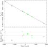 |
Fig. 3 Top panel: spin period values shown in Table 1 vs. time in units of days (see the text). The linear best fit is also plotted. The black squares, open green squares, blue diamond, and red triangle indicate the spin period values reported by Jonker & van der Klis (2001), Jain et al. (2010), Sasano et al. (2014), and this work, respectively. Bottom panel: the corresponding residuals in units of 10-6 s. |
Furthermore, we search for the same periodicity in the MOS1 data (taken in timing mode); unfortunately, the lower statistics with respect to the EPIC-pn data do not allow us to detect the periodicity in this data set.
We note that the spin period obtained from the EPIC-pn events is inconsistent with the value reported by Jain et al. (2010) using RXTE/PCA observations simultaneous to the XMM observation that we analyse in this work (see Table 1 and Fig. 3). To confirm the robustness of our results, we reanalysed the simultaneuous RXTE/PCA observations (P50048-01-01-00, 50048-01-01-01, P50048-01-01-02, P50048-01-01-03, P50048-01-01-04, P50048-01-01-05, P50048-01-01-06) spanning 2001 March 7 10:29:26 UT to 2001 March 8 4:47:44 UT. We applied the barycentric correction with respect to the source coordinates and corrected the data for the orbital motion of the binary system as done for the EPIC-pn data. No energy selection was applied to the RXTE/PCA events file. We explored the period window between 0.592384 and 0.593384 s using the FTOOL efsearch in the XRONOS package. We adopted eight phase bins per period for the trial-folded light curves and a resolution of the period search of 1 × 10⁻⁶ s. We observe a χ2 peak of 150 at 0.592884 s, as shown in Fig. 4. We fitted the peak with a Gaussian function, assumed the centroid of the Gaussian as the best estimation of the spin period, and associated the error derived from the best fit. We find that the spin period during the RXTE/PCA observations is 0.5928846(3) s and that the associated error is at the 68% confidence level. This result confirms our detection in the XMM/Epic-pn data. Finally, we note that the value of the spin period derivative obtained above does not significantly change when using our value instead of the one reported in Table 1.
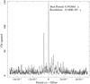 |
Fig. 4 Folding search for periodicities in the RXTE/PCA observations. The peak of χ2 is detected at 0.592884 s. |
4. Energy range selection for the XMM-Newton, Suzaku, Chandra, and INTEGRAL spectra
We rebinned the MOS1 and MOS2 spectra using the SAS tool specgroup to have at least 25 counts per energy channel and with an over-sample factor of 5. To verify that the spectra are similar and see how the pile-up effects influence the MOS2 spectrum, we fitted the two MOS spectra in the 0.6–10 keV energy range using XSPEC (version 12.8.1). We adopted a very simple model consisting of phabs*pcfabs*CompTT1, similar to the model used by Iaria et al. (2001) to fit the BeppoSAX broad-band spectrum of X1822-371. The phabs component takes the photoelectric absorption by the interstellar neutral matter into account, it is a multiplicative component defined as M(E) = exp [ −NH ∗ σ(E) ], where σ(E) is the photo-electric cross-section (not including Thomson scattering). The free parameter, NH, is the equivalent hydrogen column density in units of 1022 atoms cm-2. The pcfabs component takes the photoelectric absorption into account owing to the neutral matter near the source, and it is a multiplicative component defined as M(E) = f ∗ exp [ −NHpc ∗ σ(E) ] + (1 − f), where NHpc is the equivalent hydrogen column in units of 1022 atoms cm-2 of the local neutral matter, and f is a dimensionless free parameter ranging between 0 and 1 that takes the fraction of emitting region occulted by the local neutral matter into account.
The CompTT component (Titarchuk 1994) is a Comptonisation model of soft photons in a hot plasma. For this component, the soft photon input spectrum is a Wien law with a seed-photon temperature, kT0, that is a free parameter. The other free parameters of the component are the plasma temperature, kTe, the plasma optical depth τ, and the normalisation NCompTT. We used a slab geometry for the Comptonising cloud. We fitted the 0.6–10 keV MOS1 and MOS2 spectra simultaneously with the aim of estimating the pile-up effects in the MOS2 spectrum. We obtained a large χ2(d.o.f.) of 1716(540). The two spectra are consistent with each other between 0.6 and 7 keV. Above 7 keV the pile-up distortion is evident in the MOS2 spectrum. Furthermore, the presence of two emission lines in the residuals at 6.4 and 6.97 keV is evident; finally, both the spectra are not well fitted between 0.6 and 1 keV and show large residuals. We show the MOS1 and MOS2 residuals in Fig. 5. We sum the MOS1 and MOS2 spectra using a new recipe9. In the following the summed spectrum is called MOS12 spectrum. The MOS12 spectrum is rebinned with an over-sample factor of 5.
We added the first-order spectrum of RGS1 and RGS2 together using the SAS tool rgscombine; hereafter, the summed spectrum is called RGS12. We rebinned the RGS12 to have at least 200 counts per energy channel. In the following, we analyse the RGS12 spectrum in the 0.35–2 keV energy range.
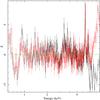 |
Fig. 5 MOS1 (black) and MOS2 (red) residuals with respect to the model described in the text. |
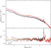 |
Fig. 6 MOS12 (0.6–7 keV; black) and EPIC-pn (0.6–10 keV; red) spectra (top panel) and ratio (data/model; bottom panel) with respect to the model described in the text. |
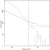 |
Fig. 7 HXD/PIN source spectrum (black) and NXB+CXB spectrum (red) are shown. The NXB+CXB spectrum overwhelms the source spectrum at energies larger than 36 keV, the energy threshold is indicated with a dashed vertical line. |
The EPIC-pn spectrum is rebinned using the SAS tool specgroup imposing at least 25 counts per energy channel and an over-sample factor of 5. To check the consistency of the EPIC-pn and MOS12 spectra, we fit them simultaneously adopting the same model described above. We obtain a large χ2(d.o.f.) value of 3228(466). We show the two spectra (MOS12 and EPIC-pn spectra) and the corresponding ratio (data/model) in Fig. 6. We observe a large absorption feature in both spectra at 0.7 keV. A mismatch between the two spectra is evident below 1.5 keV; the EPIC-pn residuals show an instrumental feature at 2.2 keV owing to the neutral gold M-edge. Finally, we detect the presence of strong emission lines in the Fe-K region. The causes of the mismatch between the EPIC-pn and MOS12 are not clear. However, we note that the residuals close to 0.7 keV are present in both the EPIC-pn and MOS12 spectra (see Fig. 6, lower panel). We adopt the 0.6–10 keV energy range for the EPIC-pn spectrum. To fit the instrumental feature at 2.2 keV in the EPIC-pn spectrum, we use an absorption Gaussian line with the centroid and the width fixed at 2.3 and 0 keV, respectively. We fit MOS12 spectrum using the 0.6–7 keV or the 1.5–7 keV energy band.
For the Suzaku/XIS data, we adopt a 0.5–10 keV energy range for the XIS0+XIS2+XIS3 (hereafter XIS023) and XIS1 spectra. We exclude the energy interval between 1.7 and 2.4 keV in the XIS023 and XIS1, because of systematic features associated with neutral silicon and neutral gold edges. We group the HXD/PIN spectrum to have 25 photons per channel and use the energy range between 15 and 36 keV. We show in Fig. 7 the HXD/PIN source spectrum and the summed HXD/PIN NXB and CXB spectra (hereafter NXB+CXB spectrum). The NXB+CXB spectrum dominates the source spectrum at energies higher than 36 keV.
We analyse the Chandra/MEG in the 0.5–7 keV energy range. Finally, we analyse the JEM-X and IBIS spectrum in the 5–22 and 21–60 keV energy band, respectively. The IBIS spectrum is background-dominated above 60 keV.
5. Spectral analysis
Best-fit values of the continuum emission.
Best-fit values of the emission lines.
We simultaneously fitted the XMM-Newton, Suzaku, Chandra, and INTEGRAL spectra. We added a systematic error of 1% to take into account that the observations are not simultaneous. Initially, we fitted the spectra using the 0.6–7 keV energy range for the MOS12.
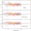 |
Fig. 8 Residuals with respect to the best-fit models shown in Tables 2 and 3. The RGS12, EPIC-pn, XIS023, XIS1, MOS12, HXD/PIN, MEG, JEM-X, and IBIS spectra are shown in black, red, green, blue, magenta, light-blue, yellow, grey, and orange, respectively. The data are graphically rebinned. From top to bottom, the residuals with respect to the continuum consist of: 1) a Comptt partially absorbed by local neutral matter (large residuals are evident at 0.7 keV); 2) gabs*Comptt with the energy of the gabs component close to 0.73 keV; 3) cyclabs*Comptt. The MOS12 spectrum covers the 0.6–7 keV energy band. |
We fitted the spectra using XSPEC version 12.8.1 (see Arnaud 1996). Initially, to fit the continuum emission, we adopted the model used by Iaria et al. (2013). It is Ed*phabs*(f*cabs*phabs*(LN+CompTT)+(1-f)* (LN+CompTT)), which is a Comptonised component (CompTT in XSPEC) absorbed by neutral interstellar matter (the first phabs component) and partially absorbed by local neutral matter (the second phabs component). We used the abundances provided by Asplund et al. (2009) and the photoelectric cross-section given by Verner et al. (1996). We took the Thomson scattering of the local neutral matter into account by adding the cabs component and imposed that the equivalent hydrogen column density of the cabs component is the same as the local neutral matter. The constant f gives the percentage of emitting region occulted by the local neutral matter. Finally, LN and Ed in the model indicate all the Gaussian components added to the model to fit the several emission lines observed in the spectrum and the added absorption edges, respectively.
Since the XMM-Newton, Suzaku, Chandra, and INTEGRAL observations are not simultaneous we left the values of the electron temperature and of the optical depth of the CompTT component free to vary independently. The depths of the absorption edges added above 7 keV were free to vary independently for the XMM-Newton, Suzaku, and INTEGRAL spectra, whilst they were tied in the Chandra spectrum to the values of the XMM-Newton spectrum because the Chandra spectrum extends up to 7 keV.
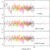 |
Fig. 9 Residuals with respect to the best-fit models shown in Tables 2 and 3. The colours are defined as in other figures. The data are graphically rebinned. From top to bottom, the residuals with respect to the continuum consist of: 1) a Comptt partially absorbed by local neutral matter (large residuals are evident at 0.7 keV); 2) gabs*Comptt with the energy of the gabs component close to 0.72 keV; 3) cyclabs*Comptt. The MOS12 spectrum covers the 1.5–7 keV energy band. |
Several emission lines are detected and identified with N vii, O vii intercombination line, O viii, Ne ix intercombination line, Ne x, Mg xi intercombination line, Mg xii, Si xiv, Fe i, and Fe xxvi. The emission lines are fitted with Gaussian components. We fixed the energies and widths of the emission lines below 6 keV at their best-fit values because their analysis is not the aim of this work; a detailed analysis of these lines is reported by Iaria et al. (2013). Finally, we added two absorption edges at 7.2 and 8.4 keV. Fitting the spectra we obtain a χ2(d.o.f.) of 3024(2496) and large residuals between 0.35 and 1 keV are visible. We show the residuals in Fig. 8 (top panel), the best-fit values of the continuum emission and absorption edges in Table 2, and the best-fit parameters associated with the emission lines in Table 3.
To fit the large residuals between 0.4 and 1 keV, we added a Gaussian absorption line (gabs in XSPEC) that is a multiplicative component. The component gabs is defined by three parameters, and its functional form is
![Mathematical equation: $$ M(E) = \exp \left[-(\tau/\sqrt{2 \pi} \sigma) \exp(-((E-E_0)/4\sigma))^2\right], $$](/articles/aa/full_html/2015/05/aa23402-14/aa23402-14-eq249.png) where τ, σ, and E0 are the line depth, the line width in keV, and the line energy in keV, respectively. We interpret this component as a CRSF in the spectrum. The model becomes Ed*phabs*(f*cabs*phabs*(LN+gC)+(1-f)*(LN+gC)), where gC is gabs*CompTT and Ed takes the absorption edges into account. The addition of the gabs component improves the fit. We obtain a χ2(d.o.f.) of 2798(2493) with a Δχ2 of 226 and a F-statistics value of 67.1. The residuals are shown in Fig. 8 (the second panel from the top). The best-fit parameters are shown in Tables 2 and 3.
where τ, σ, and E0 are the line depth, the line width in keV, and the line energy in keV, respectively. We interpret this component as a CRSF in the spectrum. The model becomes Ed*phabs*(f*cabs*phabs*(LN+gC)+(1-f)*(LN+gC)), where gC is gabs*CompTT and Ed takes the absorption edges into account. The addition of the gabs component improves the fit. We obtain a χ2(d.o.f.) of 2798(2493) with a Δχ2 of 226 and a F-statistics value of 67.1. The residuals are shown in Fig. 8 (the second panel from the top). The best-fit parameters are shown in Tables 2 and 3.
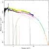 |
Fig. 10 Unfolded spectra relative to the model including the gabs component. The MOS12 spectrum ranges between 1.5 and 7 keV. Colours as above. |
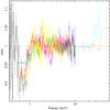 |
Fig. 11 Data/model ratio with respect to the best-fit model shown in Tables 2 and 3, but excluding the gabs component. The data are graphically rebinned. Colours as above. The MOS12 spectrum ranges between 1.5 and 7 keV. |
We also fitted the residuals between 0.4 and 1 keV using, instead of a Gaussian absorption line, an absorption line with a Lorentzian shape (Mihara et al. 1990). This multiplicative component (cyclabs in XSPEC) is defined by three parameters, and its functional form is
![Mathematical equation: $$ M(E) = \exp\left[- \tau\; (\sigma E /E_0)^2 \big/\left[(E-E_0)^2+\sigma^2\right] \right], $$](/articles/aa/full_html/2015/05/aa23402-14/aa23402-14-eq252.png) where τ, σ, and E0 are the line depth, the line width in keV, and the line energy in keV, respectively. We fixed the second harmonic depth to zero in the model. In this case the adopted model is Ed*phabs*(f*cabs*phabs*(LN+cC)+(1-f)*(LN+cC)), where cC is cyclabs*CompTT. The addition of the cyclabs component instead of the gabs component gives an equivalent fit with a χ2(d.o.f.) of 2795(2493). The best-fit values are shown in Tables 2 and 3. The residuals are shown in Fig. 8 (bottom panel).
where τ, σ, and E0 are the line depth, the line width in keV, and the line energy in keV, respectively. We fixed the second harmonic depth to zero in the model. In this case the adopted model is Ed*phabs*(f*cabs*phabs*(LN+cC)+(1-f)*(LN+cC)), where cC is cyclabs*CompTT. The addition of the cyclabs component instead of the gabs component gives an equivalent fit with a χ2(d.o.f.) of 2795(2493). The best-fit values are shown in Tables 2 and 3. The residuals are shown in Fig. 8 (bottom panel).
The residuals in Fig. 8 show that the RGS12, XIS1, XIS023, MEG, and EPIC-pn spectra are in good agreement below 1.5 keV, unlike in the MOS12 spectrum. For this reason we repeated the analysis described above excluding the 0.6–1.5 keV energy range in the MOS12 spectrum. Fitting the spectra using the initial model, we find a χ2(d.o.f.) of 2713(2466) and large residuals between 0.35 and 1 keV are visible (see Fig. 9, top panel). Using the model that includes the gabs component, we obtain a χ2(d.o.f.) of 2565(2463) with a Δχ2 of 148 and a F-statistics value of 47.4. The residuals are shown in Fig. 9 (middle panel). Using the model including the cyclabs component, we obtain a χ2(d.o.f.) of 2565(2463). The residuals are shown in Fig. 9 (bottom panel). The unfolded spectra relative to the model including the gabs component is shown in Fig. 10. We show the data/model ratio with respect to the best-fit model, but excluding the gabs component in Fig. 11.
Furthermore, using the initial model with the MOS12 spectrum between 1.5–7 keV, we look for the presence of CRSF at high energies, as suggested by Sasano et al. (2014), exploiting the availability of the JEM-X and IBIS spectra. Adding to the model a cyclabs component with width and centroid fixed to 5 keV and 33 keV (see Sasano et al. 2014), respectively, we find an upper limit on the depth of 0.10 at 99.7% confidence level (3σ). This value is not consistent with the  obtained by Sasano et al. (2014).
We find that the energy and width of the CRSF at 0.7 keV are consistent for the Lorentzian and the Gaussian shapes. The depth values of the absorption edges at 7.2 keV are compatible for the XMM-Newton and INTEGRAL spectra, while they higher in the Suzaku spectrum. Finally, the optical depth of the Comptonised component assumes similar values close to nine in the XMM-Newton, Chandra, and Suzaku spectra, while it is 6.0 ± 0.2 in the INTEGRAL spectrum.
Finally, we note that including MOS12 spectrum between 0.6 and 1.5 keV only marginally affects the fit results. In the following we use the best-fit values obtained when excluding the 0.6–1.5 keV energy range of MOS12.
6. Discussion
We used three non-simultaneous pointed X-ray observations of X1822-371: a XMM-Newton observation (using RGS, MOS, and EPIC-pn spectra), a Suzaku observation (using XIS and HXD/PIN spectra), and finally, a Chandra observation (using the first-order MEG spectrum). The spectral analysis of the XMM and Chandra data sets have already been discussed in Iaria et al. (2013). The same XMM/EPIC-pn data were also analysed by Somero et al. (2012), who report a different interpretation of the X-ray spectrum. Moreover, we used all the available INTEGRAL/JEM-X and INTEGRAL/ISGRI observations of X1822-371 and extracted the corresponding spectra to confirm or disprove a claimed CRSF at 33 keV in the Suzaku/PIN spectrum (see Sasano et al. 2014).
We adopted the same model as proposed by those authors to fit the continuum emission. It consists of a Comptonised component Comptt absorbed by interstellar matter and partially absorbed by local neutral matter. The effect of Thomson scattering on the local cold absorber is taken into account by adding the cabs component with an equivalent hydrogen column density imposed to be the same as the one associated with the local neutral matter. Iaria et al. (2013) found residuals in the EPIC-pn data between 0.6 and 0.8 keV and added a black-body component with temperature fixed to 0.06 keV, thereby improving the fit significantly.
In this work we give a different interpretation of the residuals in the EPIC-pn data between 0.4 and 1 keV, modelling them with the addition of a CRSF close to 0.7 keV. The broad residuals are fitted using the gabs or the cyclabs model components. The addition of this component significantly improves the fit, and we obtain statistically equivalent fits using either the gabs or the cyclabs component.
The interpretation of the residuals as a CRSF in the spectrum allows us to refine the scenario proposed by Iaria et al. (2013) for X1822-371. The authors suggested that the Comptonised component originates in the inner region of the system, it is not directly observable because of the large inclination angle of the system, and only 1% of its flux arrives to the observer because of scattering by an extended optically thin corona with optical depth ~0.01. We now suggest that the Comptonised component could be produced in the accretion column onto the NS magnetic caps.
Below we discuss our results showing that a CRSF at 0.7 keV agrees with the non-conservative mass transfer scenario proposed for X1822-371 in the past three years by several authors (see, for example, Iaria et al. 2013, 2011; Burderi et al. 2010; Bayless et al. 2010) and allows the NS mass of the binary system that is between 1.61 and 2.32 M⊙ to be further constrained (Muñoz-Darias et al. 2005). Burderi et al. (2010), Bayless et al. (2010), and Iaria et al. (2011) found a large orbital period derivative of X1822-371, and Burderi et al. (2010) show that this indicates that X1822-371 accretes at the Eddington limit and that the rest of the mass transferred by the companion star is expelled from the system.
Adopting the values for Ps and derived in Sect. 3 and assuming that X1822-371 accretes at its Eddington limit, we show that the CRSF energy obtained by our fits is consistent with a scenario in which the NS in X1822-371 is spinning up. Since is negative, the corotation radius rc, the radius at which the accretion disc has the same angular velocity as the NS, has to be larger than the magnetospheric radius rm, the radius at which the magnetic pressure of the NS B-field equals the ram pressure of the accreting matter. The corotation radius can be expressed as 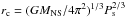 , where MNS is the NS mass and Ps is the NS spin period. Assuming a NS mass of 1.4 M⊙, we obtain rc ≃ 1180 km; for a NS mass of 2 M⊙, the corotation radius is rc ≃ 1300 km. The magnetospheric radius is given by the relation rm = φrA, where rA is the Alfvén radius and φ a constant close to 0.5 (see Ghosh & Lamb 1991). We estimate rA using the Eq. (2) in Burderi et al. (1998):
  (1)where μ30 is the magnetic moment in units of 1030 G cm3, R6 the NS radius in units of 106 cm, L37 the luminosity of the system in units of 1037 erg/s, m the NS mass in units of solar masses, and finally, ϵ is the ratio between the luminosity and the total gravitational potential energy released per second by the accreting matter.
Adopting the best-fit value of the CRSF energy, Ekev, obtained from the gabs component, and assuming that this is produced at (or very close to) the NS surface, we estimate the NS B-field using the relation Ekev = (1 + z)-111.6B12, where
 and B12 is the NS B-field in units of 1012 G. We arrange the term (1 + z)-1 in terms of m and R6 and obtain
  (2)We assume that the intrinsic luminosity of X1822-371 is the Eddington luminosity, L = 1.26 × 1038(MNS/M⊙) erg/s, which we rewrite as L37 = 12.6 m, which is the Eddington luminosity in units of 1037 erg/s. Substituting this expression of luminosity and the expression of B12 of Eq. (2) into Eq. (1) and assuming a NS radius of 10 km, we obtain
 For NS masses of 1.4 and 2 M⊙, we obtain rA ≃ 490 and ≃510 km, respectively. Since rm = φrA with φ ≃ 0.5 then for a NS mass of 1.4 and 2 M⊙, we obtain rm ≃ 245 and ≃255 km, respectively. This means that, for a NS mass between 1.4 and 2 M⊙, rm is always smaller than rc by a factor five. This implies that the accreting matter gives specific angular momentum to the NS, which increases its angular velocity and spins it up.
Next we adopt the set of relations shown by Ghosh & Lamb (1979) (Eqs. from (15) to (18)) to establish a relation for the derivative of the spin period, the spin period, the luminosity, and the NS mass. This set of equations is valid for the fastness parameter ωs = Ωs/ ΩK(ro) <ωmax ≃ 0.95, where Ωs is the NS angular velocity, ΩK(ro) is the Keplerian angular velocity at r0, and r0 is the radius that separates the boundary layer from the outer transition zone (see discussion in Ghosh & Lamb 1979). Using Eq. (2) and assuming that the NS accretes at the Eddington limit (L37 = 12.6 m), the parameter ωs of the Eq. (16) in Ghosh & Lamb (1979) becomes 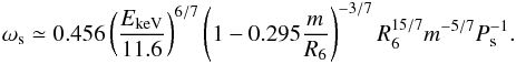 (3)Using the value of EkeV shown in Table 2, the spin period value shown in Sect. 3, and finally, imposing that R6 = 1, we find that ωs is between 0.063 and 0.083 for m between 1 and 3 M⊙. This implies that the values of NS B-field and luminosity satisfy the spin-up condition.
Using Eq. (15) of Ghosh & Lamb (1979), we constrained the NS mass. We adopted the expression of the NS moment of inertia given by Lattimer & Schutz (2005) in Eq. (16) of their work. The expression is valid for many NS equation of states and for a NS mass higher than 1 M⊙. Rewriting the expression in terms of m and R6 we obtain 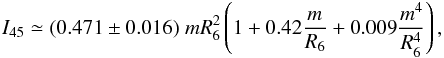 (4)where I45 is the NS moment of inertia in units of 1045 g cm2. The Eq. (15) of Ghosh & Lamb (1979) can be rewritten as
  (5)where Ṗ-12 is the spin period derivative in units of 10-12 s/s, δ is the term in parenthesis in Eq. (4), B12 is given by Eq. (2), and finally, the function n(ωs) in its useful approximate expression is
![Mathematical equation: $$ n(\omega_{\rm s}) \sim 1.39 \left\{1-\omega_{\rm s}\left[4.03(1-\omega_{\rm s})^{0.173}-0.878\right]\right\} (1-\omega_{\rm s})^{-1} $$](/articles/aa/full_html/2015/05/aa23402-14/aa23402-14-eq306.png) (see Eq. (10) in Ghosh & Lamb 1979).
(see Eq. (10) in Ghosh & Lamb 1979).
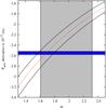 |
Fig. 12 Spin period derivative, Ṗ-12, vs. m for a NS radius of 10 km (red curve); the black curves represent the upper and lower limit values of the spin derivative. The grey box indicates the mass range allowed for X1822-371 according to Muñoz-Darias et al. (2005). The horizontal blue strip indicates the value of Ṗ-12 as derived in Sect. 3. |
Values of RNS, MNS, B, and Mc obtained from the cyclotron line energy found adopting the gabs component in the fit.
Initially, we impose that R6 = 1 and find how Ṗ-12 changes as function of m. The error associated with Ṗ-12 is mainly due to the term n(ωs), that has an accuracy of 5% (see Ghosh & Lamb 1979); we take also the errors associated with I and EkeV into account. We adopt the 1σ error for EkeV. We show the values of Ṗ-12 vs. m in Fig. 12. For a range of m between 1.3 and 2.5, the Ṗ-12 changes from –3.4 up to –1.6. The grey box in Fig. 12 limits the allowed NS mass between 1.61 and 2.32 M⊙, according to Muñoz-Darias et al. (2005). Furthermore, the value of the spin period derivative, Ṗ-12 = −2.55 ± 0.03 s/s that we obtained in Sect. 3, is shown, as are the uncertainties associated with Ṗ-12. We find a NS mass of 1.69 ± 0.13 M⊙ assuming R6 = 1, which is inside the range suggested by Muñoz-Darias et al. (2005). Consequently, using the Eq. (2), we find that the NS B-field is (8.8 ± 0.3) × 1010 G, a value that is very similar to the one suggested by Jonker & van der Klis (2001) assuming a luminosity of ~1038 erg/s for X1822-371.
Using the mass function (2.03 ± 0.03) × 10-2M⊙ and an inclination angle of X1822-371 of  (see Jonker et al. 2003), we infer the companion star mass, Mc = 0.46 ± 0.02 M⊙, which is close to the value of 0.5 M⊙ suggested by Muñoz-Darias et al. (2005). Using only optical observations, Somero et al. (2012) estimate that the mass ratio of X1822-371 is q = Mc/MNS = 0.28. Using this relation, we find that the companion star mass is Mc = 0.47 ± 0.04 M⊙ for a NS mass of 1.69 ± 0.13 M⊙, and that value is compatible with the one inferred by us using the mass function.
Assuming different NS radii for Eq. (5), we obtain different values of the NS mass. We show the NS masses for several values of the NS radius ranging from 8 to 11.5 km in Table 4. The NS radius in X1822-371 cannot be larger than 11.5 km because the NS mass would be lower than 1.61 M⊙ which is the lower limit given by Muñoz-Darias et al. (2005). This result further constrains the NS mass range between 1.46 and 1.81 M⊙. The NS B-field ranges between 7.8 and 10.5 × 10¹⁰ G, and finally, the companion star mass ranges between 0.41 and 0.48 M⊙.
We compared the results in Table 4 with those obtained by Steiner et al. (2010), which determined an empirical dense matter equation of state from a heterogeneous data set of six neutron stars: three Type-I X-ray busters with photospheric radius expansion and three transient low-mass X-ray binaries. Our comparison was done with the results reported in Table 7 by Steiner et al. (2010). They are valid for a NS radius equal to the photospheric radius of the NS. The authors find that for a NS mass of 1.6, 1.7, and 1.8 M⊙, the corresponding radius is  ,
,  , and
, and  km, respectively, with the errors at 95%. If the NS in X1822-371 is similar to those of the sample studied by Steiner et al. (2010), we can exclude from Table 4 the solutions for NS radii smaller than 9.5 km. This implies that the NS mass range is between 1.61 ± 0.15 and 1.70 ± 0.13 M⊙, that the NS B-field in units of 1010 G is between 8.1 ± 0.3 and 9.0 ± 0.3, and finally that the companion star mass is between 0.44 ± 0.03 and 0.46 ± 0.02 M⊙.
We note that the estimation of the CRSF energy is model dependent. The CRSF energy is 0.72 and 0.68 keV, adopting the gabs and cyclabs components, respectively, to fit the averaged spectrum. However, the values of the NS mass, NS magnetic-field strength, and companion star mass at different NS radii are the same as shown in Table 4 even using the CRSF energy obtained from the cyclabs component, since this energy and the NS magnetic-field strength, B12, are linearly dependent (see Eq. (2)) and because the spin period derivative weakly depends on B12 (see Eq. (5)).
The gabs component allows us to estimate the temperature of the plasma where the CRSF originates, assuming that the broadening of the line has a thermal origin. At the cyclotron resonance frequency ωc, electrons at rest absorb photons of energy ħωc. For thermal Doppler broadening, ΔωD is predicted to be (Mészáros 1992)
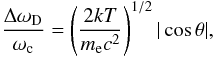 where ħΔωD = σgabs, ħωc = Egabs, kT is the electron temperature, and mec2 is the electron rest energy. The angle θ measures the direction of the magnetic field with respect to the line of sight. Outside the range ωc ± ΔωD, the cyclotron absorption coefficient decays exponentially, and other radiative processes become important. Substituting the values of σgabs and Egabs shown in Table 2 (for MOS12 spectrum ranging between 1.5 and 10 keV), we obtain a lower limit on the plasma temperature of kT = 8 ± 2 keV with the error at 68% confidence level, which is a factor of two or three larger than the electron temperature of the Comptt component, but the values are consistent at the 2σ level. This suggests that the Comptonised component is probably produced in the accretion column onto the NS magnetic caps.
We do not observe cyclotron harmonics in the spectrum. To date, the lowest energy measured for a CRSF produced by electron motion around the NS magnetic-field lines is 9 keV in the source XMMU J054134.7-682550 (Manousakis et al. 2009); also in that case, harmonics are not visible in the spectrum. The cyclotron line observed in the spectrum of the Be/X-Ray Binary Swift J1626.6-5156 has an energy of 10 keV and only a weak indication of a harmonic at 19 keV (see DeCesar et al. 2013). The source KS 1947+300 has been recently observed with Nuclear Spectroscopy Telescope Array (NuSTAR) and Swift/XRT in the 0.8–79 keV energy range (Fürst et al. 2014); a CRSF at 12.5 keV has been observed but no harmonics have been detected. Finally, the anomalous X-ray pulsar SGR 0418+5729 shows a CRSF produced by proton motion, with centroid at 1 keV, and no harmonics are observed (see Tiengo et al. 2013). To now, only the isolated NS CCO 1E1207.4-5209 shows a CRSF also and its first harmonic at 0.7 and 1.4 keV, respectively (Sanwal et al. 2002; Mereghetti et al. 2002). These results show that, although peculiar, it is possible to observe only the fundamental harmonic of the CRSF.
Finally, we note that the presence of a CRSF at 0.7 keV shown in this work contrasts with the recent result suggested by Sasano et al. (2014), who find a CRSF at 33 keV when analysing the same Suzaku data as presented in this work. First of all, we note that a CRSF at 33 keV is detectable including the HXD/PIN data up to 40 keV. However, we have shown that the HXD/PIN source spectrum is overwhelmed by the NXB+CXB spectrum at energies higher than 36 keV (see Fig. 7). Furthermore, we note that, at 33 keV, the HXD/PIN effective area is nearly 50 cm2, while the HPGSPC and PDS instruments on-board BeppoSAX had an effective area of ~200 and ~500 cm2, respectively. Iaria et al. (2001) analysed a broad band spectrum of X1822-371 using the narrow-field instruments on-board BeppoSAX and did not find any evidence of a CRSF at 30 keV with a PDS exposure time of 18.7 ks. The HXD/PIN spectrum has an exposure time of 37.7 ks, which is a factor of two longer than the PDS exposure times, but it has an effective area a factor of 10 smaller at 33 keV. The presence of a CRSF at 33 keV in the Suzaku data is therefore unrealistic when assuming that it does not change in time.
To verify the presence of a CRSF at 33 keV, we have also analysed the IBIS and JEM-X spectra for an effective dead-time-corrected exposure of 874 ks and 283 ks, respectively. We fitted both the spectra, adopting the same model as used to fit the XMM-Newton/Suzaku data and found no evidence of CRSF at 33 keV.
We also note that a CRSF at 33 keV is not consistent with the observed spin-up of the NS. Assuming that the NS is spinning-up and using the NS B-field value inferred by a CRSF at 33 keV, Sasano et al. (2014) obtain an intrinsic luminosity of the system of ~3 × 1037 erg s-1 needed to have the measured spin-up rate. In case of spin-up, we expect that the corotation radius rc has to be larger than the magnetospheric radius rm. The values of rc is 1180 km and 1300 km for a NS mass of 1.4 and 2 M⊙, respectively, assuming the value reported by Sasano et al. (2014) as spin period. To estimate the magnetospheric radius, we used the Eq. (1) assuming a NS radius of 10 km and a NS B-field of 2.8 × 10¹² G (see Sasano et al. 2014). For a NS mass of 1.4 M⊙, we find that rA ≃ 5940 km and rm = φrA ≃ 3000 km, with φ = 0.5. We infer that rm ≃ 3rc, and this implies that matter cannot accrete onto the NS; this scenario corresponds to that discussed by Ghosh & Lamb (1979) for ωs ≫ ωmax with ωmax ≃ 0.95. In fact,
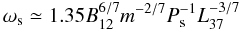 for a NS radius of 10 km (see Eqs. (16) and (18) in Ghosh & Lamb 1979). Using the values of luminosity, spin period, and NS B-field reported by Sasano et al. (2014), we find that ωs ≃ 3.2 for a NS mass of 1.3 M⊙ and ≃2.5 for 3 M⊙. This result suggests that the scenario is not self-consistent because the values of luminosity and NS B-field would contradict the observed spin-up of the NS.
7. Conclusion
We analysed the broadband X-ray spectrum of X1822-371 using all the presently available data sets that allow for high-resolution spectroscopic studies. Our aim was to understand the nature of the residuals between 0.6 and 0.8 keV previously observed in the XMM/EPIC-pn data by Iaria et al. (2013). Initially, we analysed the averaged spectra simultaneously. The broad band spectrum obtained from Suzaku constrains the continuum emission well. The adopted model was a Comptonised component absorbed by the neutral interstellar matter and partially absorbed by local neutral matter. We took the Thomson scattering into account and fixed the value of the equivalent hydrogen column density of the local neutral matter to that producing the Thomson scattering.
The values of the parameters are similar for the three data sets and consistent with previous studies (see e.g. Iaria et al. 2013). To fit the residuals between 0.6 and 0.8 keV, we added an absorption feature with Gaussian profile (gabs in XSPEC). Alternatively, we adopted an absorbing feature with Lorentzian profile (cyclabs in XSPEC). In both cases the addition of a CRSF to the model improved the fit. We found that the improvement does not depend sensitively on the exact shape used to model the absorption profile.
We also detected the spin period of X1822-371 in the EPIC-pn data. We obtained the value of 0.5928850(6) s. Using all the measurements known of the spin period of X1822-371, we estimated that the spin period derivative of the source is −2.55(3) × 10-12 s/s, and this confirms that the neutron star is spinning up. Folding the EPIC-pn light curve, we derived a pulse fraction of 0.75% in the 2–5.4 keV energy band.
Using the best-fit values of the CRSF parameters, under the assumption that the system is accreting at the Eddington limit, we estimate a NS B-field between (8.1 ± 0.3) × 1010 and (9.0 ± 0.3) × 1010 G for a NS radius ranging between 9.5 and 11.5 km. We subsequently constrain the NS mass assuming that the CRSF is produced at the NS surface. We find that, for a Gaussian profile of the CRSF, the NS mass is between 1.61 ± 0.15 and 1.70 ± 0.13 M⊙. The companion star mass is constrained between 0.44 ± 0.03 and 0.46 ± 0.02 M⊙.
Finally, we note that our conclusions contrast with the recent results reported by Sasano et al. (2014), who report detecting a CRSF at 33 keV (and a corresponding NS-B field of 3 × 10¹² G) in the Suzaku data also used in this work. To address this point, we have selected the whole IBIS and JEM-X public data set of the X1822-371 region. We extracted the JEM-X and IBIS spectra of X1822-371 having an exposure time of 330 and 874 ks, respectively. The INTEGRAL spectrum combined with the XMM, Suzaku, and Chandra spectra does not show a CRSF at 33 keV. Furthermore, we also show from theoretical arguments that a CRSF at 33 keV is not consistent with the evidence that the NS in X1822-371 is spinning up.
The names of the cited spectral models are consistent with those adopted in the spectral fitting package XSPEC (Arnaud 1996). The models are described in http://heasarc.gsfc.nasa.gov/xanadu/xspec/manual/XspecModels.html
See http://heasarc.gsfc.nasa.gov/docs/suzaku/analysis/suzaku_ftools.html for more details.
The JEM-X2 unit was active only during a limited part of the mission, so the exposure time is not enough to provide a significant spectral constraint.
Acknowledgments
The High-Energy Astrophysics Group of Palermo acknowledges support from the Fondo Finalizzato alla Ricerca (FFR) 2012/13, project No. 2012-ATE-0390, founded by the University of Palermo. This work was partially supported by the Regione Autonoma della Sardegna through POR-FSE Sardegna 2007-2013, L.R. 7/2007, Progetti di Ricerca di Base e Orientata, Project No. CRP-60529, and by the INAF/PRIN 2012-6. A.R. gratefully acknowledges Sardinia Regional Government for the financial support (P.O.R. Sardegna F.S.E. Operational Programme of the Autonomous Region of Sardinia, European Social Fund 2007-2013 – Axis IV Human Resources, Objective l.3, Line of Activity l.3.1).
References
- Arnaud, K. A. 1996, in Astronomical Data Analysis Software and Systems V, eds. G. H. Jacoby, & J. Barnes, ASP Conf. Ser. 101, 17 [Google Scholar]
- Asplund, M., Grevesse, N., Sauval, A. J., & Scott, P. 2009, ARA&A, 47, 481 [NASA ADS] [CrossRef] [Google Scholar]
- Bayless, A. J., Robinson, E. L., Hynes, R. I., Ashcraft, T. A., & Cornell, M. E. 2010, ApJ, 709, 251 [NASA ADS] [CrossRef] [Google Scholar]
- Boldt, E. 1987, in Observational Cosmology, eds. A. Hewitt, G. Burbidge, & L. Z. Fang, IAU Symp., 124, 611 [Google Scholar]
- Brinkman, A., Aarts, H., den Boggende, A., et al. 1998, in Science with XMM Conf. held at ESTEC, Noordwijk, The Netherlands, Sep. 30–Oct. 2, http://xmm.esac.esa.int/external/xmm_science/workshops/1st_workshop, article #2 [Google Scholar]
- Burderi, L., di Salvo, T., Robba, N. R., et al. 1998, ApJ, 498, 831 [NASA ADS] [CrossRef] [Google Scholar]
- Burderi, L., di Salvo, T., Riggio, A., et al. 2010, A&A, 515, A44 [NASA ADS] [CrossRef] [EDP Sciences] [Google Scholar]
- Courvoisier, T. J.-L., Walter, R., Beckmann, V., et al. 2003, A&A, 411, L53 [NASA ADS] [CrossRef] [EDP Sciences] [Google Scholar]
- Cui, W. 1997, ApJ, 482, L163 [NASA ADS] [CrossRef] [Google Scholar]
- DeCesar, M. E., Boyd, P. T., Pottschmidt, K., et al. 2013, ApJ, 762, 61 [NASA ADS] [CrossRef] [Google Scholar]
- den Herder, J. W., Brinkman, A. C., Kahn, S. M., et al. 2001, A&A, 365, L7 [NASA ADS] [CrossRef] [EDP Sciences] [Google Scholar]
- Fürst, F., Pottschmidt, K., Wilms, J., et al. 2014, ApJ, 784, L40 [NASA ADS] [CrossRef] [Google Scholar]
- Ghosh, P., & Lamb, F. K. 1979, ApJ, 234, 296 [NASA ADS] [CrossRef] [Google Scholar]
- Ghosh, P., & Lamb, F. K. 1991, Neutron Stars: Theory and Observation, Proc. NATO Advanced Study Institute on Neutron Stars: an Interdisciplinary Field, Agia Pelagia, Crete, Greece, September 3–14, Nato ASI series (Kluwer Academic Publishers), 363 [Google Scholar]
- Heinz, S., & Nowak, M. A. 2001, MNRAS, 320, 249 [NASA ADS] [CrossRef] [Google Scholar]
- Hellier, C., & Mason, K. O. 1989, MNRAS, 239, 715 [NASA ADS] [CrossRef] [Google Scholar]
- Iaria, R., Di Salvo, T., Burderi, L., & Robba, N. R. 2001, ApJ, 557, 24 [NASA ADS] [CrossRef] [Google Scholar]
- Iaria, R., di Salvo, T., Burderi, L., et al. 2011, A&A, 534, A85 [NASA ADS] [CrossRef] [EDP Sciences] [Google Scholar]
- Iaria, R., Di Salvo, T., D’Aì, A., et al. 2013, A&A, 549, A33 [NASA ADS] [CrossRef] [EDP Sciences] [Google Scholar]
- Jain, C., Paul, B., & Dutta, A. 2010, MNRAS, 409, 755 [NASA ADS] [CrossRef] [Google Scholar]
- Jonker, P. G., & van der Klis, M. 2001, ApJ, 553, L43 [NASA ADS] [CrossRef] [Google Scholar]
- Jonker, P. G., van der Klis, M., & Groot, P. J. 2003, MNRAS, 339, 663 [NASA ADS] [CrossRef] [Google Scholar]
- Koyama, K., Tsunemi, H., Dotani, T., et al. 2007, PASJ, 59, 23 [Google Scholar]
- Lattimer, J. M., & Schutz, B. F. 2005, ApJ, 629, 979 [NASA ADS] [CrossRef] [Google Scholar]
- Lebrun, F., Leray, J. P., Lavocat, P., et al. 2003, A&A, 411, L141 [NASA ADS] [CrossRef] [EDP Sciences] [Google Scholar]
- Lund, N., Budtz-Jørgensen, C., Westergaard, N. J., et al. 2003, A&A, 411, L231 [NASA ADS] [CrossRef] [EDP Sciences] [Google Scholar]
- Manousakis, A., Walter, R., Audard, M., & Lanz, T. 2009, A&A, 498, 217 [NASA ADS] [CrossRef] [EDP Sciences] [Google Scholar]
- Mereghetti, S., De Luca, A., Caraveo, P. A., et al. 2002, ApJ, 581, 1280 [NASA ADS] [CrossRef] [Google Scholar]
- Mészáros, P. 1992, High-energy radiation from magnetized neutron stars (Chicago: Univ. Chicago Press) [Google Scholar]
- Mihara, T., Makishima, K., Ohashi, T., Sakao, T., & Tashiro, M. 1990, Nature, 346, 250 [NASA ADS] [CrossRef] [Google Scholar]
- Muñoz-Darias, T., Casares, J., & Martínez-Pais, I. G. 2005, ApJ, 635, 502 [NASA ADS] [CrossRef] [Google Scholar]
- Papitto, A., D’Aì, A., Motta, S., et al. 2011, A&A, 526, L3 [Google Scholar]
- Parmar, A. N., Oosterbroek, T., Del Sordo, S., et al. 2000, A&A, 356, 175 [NASA ADS] [Google Scholar]
- Sanwal, D., Pavlov, G. G., Zavlin, V. E., & Teter, M. A. 2002, ApJ, 574, L61 [NASA ADS] [CrossRef] [Google Scholar]
- Sasano, M., Makishima, K., Sakurai, S., Zhang, Z., & Enoto, T. 2014, PASJ, 66, 35 [NASA ADS] [Google Scholar]
- Somero, A., Hakala, P., Muhli, P., Charles, P., & Vilhu, O. 2012, A&A, 539, A111 [NASA ADS] [CrossRef] [EDP Sciences] [Google Scholar]
- Steiner, A. W., Lattimer, J. M., & Brown, E. F. 2010, ApJ, 722, 33 [NASA ADS] [CrossRef] [Google Scholar]
- Strüder, L., Briel, U., Dennerl, K., et al. 2001, A&A, 365, L18 [NASA ADS] [CrossRef] [EDP Sciences] [Google Scholar]
- Takahashi, T., Abe, K., Endo, M., et al. 2007, PASJ, 59, 35 [NASA ADS] [CrossRef] [EDP Sciences] [Google Scholar]
- Tiengo, A., Esposito, P., Mereghetti, S., et al. 2013, Nature, 500, 312 [NASA ADS] [CrossRef] [PubMed] [Google Scholar]
- Titarchuk, L. 1994, ApJ, 434, 570 [NASA ADS] [CrossRef] [Google Scholar]
- Turner, M. J. L., Abbey, A., Arnaud, M., et al. 2001, A&A, 365, L27 [NASA ADS] [CrossRef] [EDP Sciences] [Google Scholar]
- Ubertini, P., Lebrun, F., Di Cocco, G., et al. 2003, A&A, 411, L131 [NASA ADS] [CrossRef] [EDP Sciences] [Google Scholar]
- Verner, D. A., Ferland, G. J., Korista, K. T., & Yakovlev, D. G. 1996, ApJ, 465, 487 [NASA ADS] [CrossRef] [Google Scholar]
- Winkler, C., Courvoisier, T. J.-L., Di Cocco, G., et al. 2003, A&A, 411, L1 [NASA ADS] [CrossRef] [EDP Sciences] [Google Scholar]
All Tables
Values of RNS, MNS, B, and Mc obtained from the cyclotron line energy found adopting the gabs component in the fit.
All Figures
|
Fig. 1 Folding search for periodicities in the 2–5.4 keV EPIC-pn light curve. We adopt 8 phase bins per period for the trial-folded light curves and a resolution of period search of 1 × 10⁻⁶ s. The peak of χ2 is detected at 0.592884 s. The horizontal dashed line indicate the χ2 value of 18.47 at which we have the 99% confidence level for a single trial. |
| In the text | |
|
Fig. 2 EPIC-pn folded light curves of X1822-371 using the folding period 0.5928850(6) s. The folded light curve is obtained using 16 phase bins per period. |
| In the text | |
|
Fig. 3 Top panel: spin period values shown in Table 1 vs. time in units of days (see the text). The linear best fit is also plotted. The black squares, open green squares, blue diamond, and red triangle indicate the spin period values reported by Jonker & van der Klis (2001), Jain et al. (2010), Sasano et al. (2014), and this work, respectively. Bottom panel: the corresponding residuals in units of 10-6 s. |
| In the text | |
|
Fig. 4 Folding search for periodicities in the RXTE/PCA observations. The peak of χ2 is detected at 0.592884 s. |
| In the text | |
|
Fig. 5 MOS1 (black) and MOS2 (red) residuals with respect to the model described in the text. |
| In the text | |
|
Fig. 6 MOS12 (0.6–7 keV; black) and EPIC-pn (0.6–10 keV; red) spectra (top panel) and ratio (data/model; bottom panel) with respect to the model described in the text. |
| In the text | |
|
Fig. 7 HXD/PIN source spectrum (black) and NXB+CXB spectrum (red) are shown. The NXB+CXB spectrum overwhelms the source spectrum at energies larger than 36 keV, the energy threshold is indicated with a dashed vertical line. |
| In the text | |
|
Fig. 8 Residuals with respect to the best-fit models shown in Tables 2 and 3. The RGS12, EPIC-pn, XIS023, XIS1, MOS12, HXD/PIN, MEG, JEM-X, and IBIS spectra are shown in black, red, green, blue, magenta, light-blue, yellow, grey, and orange, respectively. The data are graphically rebinned. From top to bottom, the residuals with respect to the continuum consist of: 1) a Comptt partially absorbed by local neutral matter (large residuals are evident at 0.7 keV); 2) gabs*Comptt with the energy of the gabs component close to 0.73 keV; 3) cyclabs*Comptt. The MOS12 spectrum covers the 0.6–7 keV energy band. |
| In the text | |
|
Fig. 9 Residuals with respect to the best-fit models shown in Tables 2 and 3. The colours are defined as in other figures. The data are graphically rebinned. From top to bottom, the residuals with respect to the continuum consist of: 1) a Comptt partially absorbed by local neutral matter (large residuals are evident at 0.7 keV); 2) gabs*Comptt with the energy of the gabs component close to 0.72 keV; 3) cyclabs*Comptt. The MOS12 spectrum covers the 1.5–7 keV energy band. |
| In the text | |
|
Fig. 10 Unfolded spectra relative to the model including the gabs component. The MOS12 spectrum ranges between 1.5 and 7 keV. Colours as above. |
| In the text | |
|
Fig. 11 Data/model ratio with respect to the best-fit model shown in Tables 2 and 3, but excluding the gabs component. The data are graphically rebinned. Colours as above. The MOS12 spectrum ranges between 1.5 and 7 keV. |
| In the text | |
|
Fig. 12 Spin period derivative, Ṗ-12, vs. m for a NS radius of 10 km (red curve); the black curves represent the upper and lower limit values of the spin derivative. The grey box indicates the mass range allowed for X1822-371 according to Muñoz-Darias et al. (2005). The horizontal blue strip indicates the value of Ṗ-12 as derived in Sect. 3. |
| In the text | |
Current usage metrics show cumulative count of Article Views (full-text article views including HTML views, PDF and ePub downloads, according to the available data) and Abstracts Views on Vision4Press platform.
Data correspond to usage on the plateform after 2015. The current usage metrics is available 48-96 hours after online publication and is updated daily on week days.
Initial download of the metrics may take a while.