| Issue |
A&A
Volume 576, April 2015
|
|
|---|---|---|
| Article Number | L3 | |
| Number of page(s) | 4 | |
| Section | Letters | |
| DOI | https://doi.org/10.1051/0004-6361/201525854 | |
| Published online | 16 March 2015 | |
Towards DIB mapping in galaxies beyond 100 Mpc
A radial profile of the λ5780.5 diffuse interstellar band in AM 1353-272 B⋆
1 GEPI, Observatoire de Paris, CNRS, Université Paris-Diderot, Place Jules Janssen, 92190 Meudon, France
e-mail: ana.monreal-ibero@obspm.fr
2 Leibniz-Institut für Astrophysik Potsdam (AIP), An der Sternwarte 16, 14482 Potsdam, Germany
3 Institut für Physik und Astronomie, Universität Potsdam, 14476 Golm, Germany
4 European Southern Observatory, 3107 Alonso de Córdova, Santiago, Chile
5 Leiden Observatory, Leiden University, PO Box 9513, 2300 RA Leiden, The Netherlands
6 Institut für Astrophysik, Universität Göttingen, Friedrich-Hund-Platz 1, 37077 Göttingen, Germany
Received: 10 February 2015
Accepted: 20 February 2015
Context. Diffuse interstellar bands (DIBs) are non-stellar weak absorption features of unknown origin found in the spectra of stars viewed through one or several clouds of the interstellar medium (ISM). Research of DIBs outside the Milky Way is currently very limited. In particular, spatially resolved investigations of DIBs outside of the Local Group are, to our knowledge, inexistent.
Aims. In this contribution, we explore the capability of the high-sensitivity integral field spectrograph, MUSE, as a tool for mapping diffuse interstellar bands at distances larger than 100 Mpc.
Methods. We used MUSE commissioning data for AM 1353-272 B, the member with the highest extinction of the Dentist’s Chair, an interacting system of two spiral galaxies. High signal-to-noise spectra were created by co-adding the signal of many spatial elements distributed in a geometry of concentric elliptical half-rings.
Results. We derived decreasing radial profiles for the equivalent width of the λ5780.5 DIB both in the receding and approaching side of the companion galaxy up to distances of ~4.6 kpc from the centre of the galaxy. The interstellar extinction as derived from the Hα/Hβ line ratio displays a similar trend, with decreasing values towards the external parts. This translates into an intrinsic correlation between the strength of the DIB and the extinction within AM 1353-272 B, consistent with the currently existing global trend between these quantities when using measurements for Galactic and extragalactic sightlines.
Conclusions. It seems feasible to map the DIB strength in the Local Universe, which has up to now only been performed for the Milky Way. This offers a new approach to studying the relationship between DIBs and other characteristics and species of the ISM in addition to using galaxies in the Local Group or sightlines towards very bright targets outside the Local Group.
Key words: dust, extinction / ISM: lines and bands / galaxies: ISM / galaxies: individual: AM1353-272 B
© ESO, 2015
1. Introduction
Diffuse interstellar bands (DIBs) are non-stellar weak absorption features found in the spectra of stars viewed trough one or several clouds of the interstellar medium (ISM, Herbig 1995). They were identified for the first time by Heger (1922), but their interstellar origin was established in the 1930s (Merrill 1934). Almost one century after their discovery, the nature of their carriers (i.e. the agent that causes these features) remains a mystery (Fulara & Krełowski 2000). However, several of the DIBs are relatively strong and present good correlations with the amount of neutral hydrogen, the extinction, and the interstellar Na I D and Ca H and K lines along a given line of sight (e.g. Herbig 1993; Friedman et al. 2011). Thus, irrespective of the actual nature of carriers, DIBs can be used as tools to infer the properties of the ISM structure, as shown by several recent works for the Milky Way (e.g. Puspitarini et al. 2015; Zasowski et al. 2015; Kos et al. 2014; Cordiner et al. 2013).
Equivalent examples for other galaxies are difficult to find. There is a certain level of spatial resolution in the investigations of DIBs in galaxies within the Local Group (Ehrenfreund et al. 2002; Cordiner et al. 2011; van Loon et al. 2013), since several sightlines in a given galaxy are sampled. Works targeting DIBs outside the Local Group are still rare and address individual sightlines for a given target (e.g. Heckman & Lehnert 2000; Phillips et al. 2013). Currently, no mapping of a DIB has been performed for galaxies outside of the Local Group (beyond ~1 Mpc).
The advent of highly efficient integral field units renders this feasible for the first time. They simultaneously record the spatially resolved spectral information in an extended continuous field. This can be tessellated a posteriori, preserving the relevant spatial information as best possible, but at the same time optimizing the quality of the signal by co-adding the spectra belonging to a given portion of the mapped area – the tile – (e.g. Monreal-Ibero et al. 2005; Sandin et al. 2008). Here, we use this principle to explore the capabilities of MUSE to obtain spatially resolved information of extragalactic DIBs.
We carried out our experiment in the interacting system AM 1353-272. The system consists of two components. The main galaxy (A) presents two prominent ~40 kpc long tidal tails and was thoroughly studied by Weilbacher et al. (2000, 2002, 2003). The companion (B) is a low-luminosity (MB = −18.1 mag) disk-like galaxy of disturbed morphology undergoing a strong starburst and with high extinction. The relative positions of A and B are shown in Fig. 1 of Weilbacher et al. (2002). Here, we used AM 1353-272 B as a test bench to explore the possibility of DIB detection and mapping. We assume a distance of D = 159 Mpc for AM 1353-272 using H0 = 75 km s-1, as in Weilbacher et al. (2002). This implies a linear scale of a 0.771 kpc arcsec-1.
2. Observations and data reduction
The interacting system AM 1353-272 was observed as part of commissioning run 2a (Bacon et al. 2014) of the MUSE instrument at the VLT. Six 900 s exposures were taken in two positions between 2014-04-29T04:22:00 and 06:00 under conditions of a few thin clouds and an average effective airmass of 1.04. The seeing as given by the Gaussian FWHM of the stars in the white-light image of the final cube is 0.̋8. Each position was observed at position angles (PA) of 0°, 90°, and 180°. The instrument was set to wide-field mode (~1′ × 1′ field of view) with a nominal wavelength range (~4800 ...9300 Å). The instrument resolution at 7000 Å is R ~ 2800. The standard star GJ 754.1A was observed on 2014-04-28T09:57:00, and the reduction made use of twilight skyflats taken on 2014-04-27.
Standard reduction steps were followed with MUSE pipeline v1.0 (Weilbacher et al. 2014), with bias subtraction, flat-fielding, and spectral tracing using the lamp-flat exposures, wavelength calibration, all using standard daytime calibration exposures made the morning after the observations. The standard geometry table and astrometric solution for commissioning run 2a were used to then transform the science data into pixel tables. This last step included correction for atmospheric refraction, flux calibration, and sky subtraction. The sky spectrum was measured in the blank areas of each exposure, set to the darkest 40% of the field of view, and data were corrected to barycentric velocities, resulting in corrections of –0.6 to –0.7 km s-1 for the time of observations. The final, combined datacube was then reconstructed from all six exposures, sampling the data at  , rejecting cosmic rays in the process. We used a subset of 111 × 91 spatial elements for the experiment presented here.
3. Extracting information
3.1. Tile definition
The galaxy has receding and approaching velocities at the southeast and northwest side, respectively (Weilbacher et al., in prep.). Since the velocity gradient is strong (Δv ≳ 300 km s-1), we treated each side of the galaxy independently, this way avoiding a large artificial broadening of the spectral features. To do this, the tiles were defined as elliptical half rings following the morphology of the galaxy, with a fixed PA = 153°, measured counterclockwise, relative to the north, and an ellipticity of b/a = 0.2. The ring sizes represent a compromise between retaining as much spatial resolution as possible and having a reliable DIB detection. The final tiles (depicted in Fig. 1) have between 29 and 159 spatial elements each (projected areas between 0.7 and 3.8 kpc2).
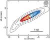 |
Fig. 1 Apertures used to extract the high signal-to-noise spectra (i.e. the tiles). Each tile has been coloured differently using a palette that follows the blue-to-red velocity distribution within the galaxy. As a reference, the reconstructed white-light image is overplotted as contours in logarithmic stretching with 0.25 dex steps. |
3.2. Feature fitting
The spectra belonging to each tile were co-added, extracted, and corrected from a Galactic extinction of Av = 0.165 (Schlafly & Finkbeiner 2011) using the IRAF task deredden and assuming RV = A(V) /E(B − V) = 3.1 (Rieke & Lebofsky 1985). In each spectrum, we fitted different spectral features needed for our analysis using the IDL-based routine mpfit (Markwardt 2009). The results discussed here are based on the equivalent width of the DIB at λ5780.5 (EW(λ5780.5)), and fluxes for Hα, Hβ, [O iii]λ5007, and [N ii]λ6584. We refer to Monreal-Ibero et al. (2010) for a description of the information recovery for the emission lines since it is quite standard and not particularly challenging for the experiment described here.
The most critical feature is the DIB at λ5780.5. This was fitted together with the sodium doublet at λλ5889.9, 5895.9 and the He iλ5876 emission line using Gaussian functions, fixing their relative central positions according to a redshift of z = 0.039467 (v = 11 840 km s-1 ), as determined from the average of the Hα centroid in the two inner half rings and in accord with the 11 790 ± 50 km s-1 reported by Weilbacher et al. (2003) and with same line width. Additionally, we included a one-degree polynomial to model the stellar continuum. The DIB at λ5797.1 was not included in the fit since we did not see any evidence for it in our spectra. It is known that the ratio of the equivalent width of these two DIBs can vary up to a factor ~5, depending on the characteristics of the ISM in the sight line of consideration (Vos et al. 2011), but only in very specific situations both DIBs are comparable. Typically, the DIB λ5797.1 is ~3–5 times fainter.
Figure 2 shows the six fits for this critical range. The DIB at λ5780.5 is clearly seen in all of them, with the possible exception of the outermost approaching half-ring. Hereafter, error bars indicate a preliminary estimate of the uncertainties as derived using Eq. (1) in Monreal-Ibero et al. (2011), which takes into account the signal-to-noise ratio of the spectra. However, the greatest source of uncertainty is the possible contamination in the spectra by a stellar spectral feature at λ5782, rest frame, with contributions from Fe i, Cr i, Cu i, and Mg i (Worthey et al. 1994), and whose strength increases with age and metallicity. An in-depth study to model this feature is beyond the scope of this initial experiment. In the following we discuss the expected maximum amount of contamination and provide an ad hoc correction for it.
We measured EW(Hα) in emission varying from ~90 Å in the inner rings to ~60 Å in the outer ones, which points to a very young (i.e. ≲7 Myr) underlying stellar population. The ages of the star-forming knots in AM 1353-272 A (≲40 Myr, Weilbacher et al. 2000), as indicative of the moment when the interaction triggered the star formation would be another way to estimate the age of the stars in AM 1353-272 B. Likewise, using the N2 and O3N2 calibrators and the expressions provided by Marino et al. (2013), we estimate a metallicity for the inner rings of 12 + log (O/H) = 8.50 and 8.42, respectively (i.e. about half solar), decreasing outwards. To estimate an upper limit for the contamination of the stellar feature, we conservatively created 1000 mock spectra by taking the spectrum of a 60 Myr single stellar population from the MILES library with solar metallicity (Falcón-Barroso et al. 2011), adding Gaussians representing the DIBs at λ5780.5 and λ5797.1 and the He iλ5876 emission line. Then, we added noise with a scale of the standard deviation between 5020 Å and 5040 Å, rest-frame. EW(λ5780.5) in the spectra was varied between 10 mÅ and 735 mÅ. As discussed above, a common range for the relative strength of the two DIBs is ~3–5. Here, we assumed EW(λ5797.1) = EW(λ5780.5)/3. We measured EW(λ5780.5) in these mock spectra using the same methodology as in the real data. The relation between input and output equivalent widths was fitted to a one-degree polynomial that was used to estimate an upper limit to the correction due to the stellar feature contamination. Measured EW(λ5780.5) ≲ 200 mÅ are consistent with no DIB, EW(λ5780.5) ~ 300 mÅ should be reduced by a 40%. For EW(λ5780.5) ≳ 500 mÅ a reduction of ~20% is enough. This simulation also suggests that under typical conditions, an EW(λ 5780.5) ≳ 800 mÅ would be necessary to have some expectations for detecting the DIB at λ5797.1.
4. Results
4.1. Radial profiles
The upper plot of Fig. 3 shows EW(λ5780.5) as a function of the semimajor axis. The receding and approaching halves of the galaxy both present a negative gradient of the DIB strength with distance to the centre. This points towards a direct link with the intrinsic properties of the galaxy.
One of the best established correlations between DIB strength and other characteristics of the ISM is that with the interstellar extinction (Herbig 1993). We derived an estimate of the extinction using the extinction curve of Fluks et al. (1994) and assuming an intrinsic Balmer emission-line ratio Hα/Hβ = 2.86 for a case B aproximation and Te = 10 000 K (Osterbrock & Ferland 2006). The corresponding radial profiles are shown in the lower plot of Fig. 3. As with the DIB, they display a decreasing gradient towards larger distances from the centre of the galaxy. This implies an intrinsic correlation between extinction and EW(λ5780.5) for AM1353-272 B and further supports the derived radial profiles for the DIB.
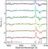 |
Fig. 2 Spectra for the six half rings showing the fit in the area of the DIB, ordered from smallest top to largest bottom velocity and normalized to the median in the displayed spectral range. The expected locations of the discussed features are marked at the bottom of the figure. The colour code in the fits echoes the ordering in velocity. Likewise, the shift of the spectral features is clearly visible. |
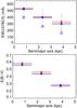 |
Fig. 3 Radial profiles for EW(λ5780.5) (top) and the extinction (bottom) as derived from Hα/Hβ for the approaching (stars and blue lines) and receding (circles and red lines) sides. The horizontal bars traversing the filled symbols mark the radial extent over which the spectra were co-added. In the upper plot, filled symbols indicate measurements without correction, while open symbols include the maximum correction for the contamination of the stellar feature at λ5782 Å. |
4.2. Comparison with other sightlines
Figure 4 illustrates the comparison between this intrinsic correlation with measurements for other sightlines. The sample is by no means complete, but covers a diversity of environments, methodologies, sampled areas, etc. This includes examples of spatially resolved measurements of the two large spirals in the Local Group (Puspitarini et al. 2013; Cordiner et al. 2011) as well as for the Magellanic Clouds (Welty et al. 2006). Likewise, we included some supernovae (Phillips et al. 2013) and nearby galaxies (Heckman & Lehnert 2000). There is a clear correlation between extinction and EW(λ5780.5). Specifically, the ratio between this two quantities across AM 1353-272 B is constant (within experimental errors), despite variations in metallicity, radiation field, etc. (Weilbacher et al., in prep.). When examining the ensemble of data globally, the dispersion is larger, pointing at secondary parameters modulating this correlation. In particular, for a given reddening, DIBs in the Magellanic Clouds are a factor 2–6 fainter than Galactic sightlines, as pointed out by Welty et al. (2006). All of our measurements in AM 1353-272 B agree well with this general relation. Interestingly enough, the relation between EW(λ5780.5) and E(B − V) is tighter when only resolved studies of disk-like galaxies are taken into account (Milky Way, Andromeda, our data). AM 1353-272 B indeed occupies an extension towards high EWs and E(B − V) of the relation found for the large spirals in the Local Group.
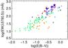 |
Fig. 4 Relation between EW(λ5780.5) and extinction for AM1353-272 (red circles and blue stars). Symbols and colours are as in Fig. 3. Additionally, we show the following Galactic (triangles) and extragalactic (inverted triangles) sightlines: green (Milky Way, Puspitarini et al. 2013); purple (M 31, Cordiner et al. 2011), orange (Magellanic Clouds, Welty et al. 2006), light blue (supernovae, Phillips et al. 2013), black (dusty starbursts, Heckman & Lehnert 2000). We used filled symbols when a galaxy had spatially resolved detections and open symbols when there is a single sightline for a given target. |
5. Summary and perpectives
This work presents the first spatially resolved detection of a DIB in a galaxy outside the Local Group. By using 568 MUSE spectra sampling a total projected area of 13.5 kpc2, we were able to measure the equivalent width of the DIB at λ5780.5 in six locations of AM 1353-272 B. Our strategy constitutes an alternative approach to extragalactic DIB studies different from using targets in the Local Group and individual sightlines outside the Local Group. We found three main results:
-
1.
We found decreasing radial profiles for EW(λ5780.5), both in thereceding and approaching sides ofAM 1353-272 B up todistances of ~4.6 kpc from the galaxy centre.
-
2.
The interstellar extinction displays a similar trend, with decreasing values towards the external parts. This translates into a correlation between the strength of the DIB and the extinction within AM 1353-272 B.
-
3.
A comparison of E(B − V) and EW(λ5780.5) in AM 1353-272 B and other sightlines shows that this intrinsic correlation agrees with the existing global trend between these quantities, especially when compared with targets in the spiral galaxies of the Local Group (i.e. our Galaxy and M 31).
When seen globally, these three results demonstrate that the spatially resolved detection of DIBs in galaxies outside the Local Group is possible and 2D DIB mapping feasible thanks to high-sensitivity instruments like MUSE. There are currently no 2D maps of DIBs in galaxies other than the Milky Way. The construction of such maps will permit studying the relationship between the DIBs and other components of the ISM in conditions different from those found in our Galaxy. We will be able to address questions like whether an extinction-DIB correlation in extremely dense environments also exists, to which degree the strength of the different DIBs depends on the dust-to-gas ratio, how DIBs react to the radiation field typical of an environment of extreme star formation, or whether the different relations locally found (e.g. the various DIB families) also exist in other galaxies, and how they depend on the intrinsic characteristics of the galaxies (e.g. morphology, metallicity, etc.). The answers will be a critical test that will help to constrain the nature of the carriers.
Acknowledgments
We thank the referee for the diligent reading of the manuscript as well as for providing valuable comments that helped us to clarify and improve the first submitted version of this Letter. We thank the MUSE collaboration and PI R. Bacon for building this extraordinary spectrograph and the rest of the commissioning team, G. Zins in particular, for the tireless effort to continue improving the instrument through all runs. A.M.-I. and R.L. acknowledge support from Agence Nationale de la Recherche through the STILISM project (ANR-12-BS05-0016-02). P.M.W. and S.K. received support through BMBF Verbundforschung (project MUSE-AO, grants 05A14BAC and 05A14MGA).
References
- Bacon, R., Vernet, J., Borisiva, E., et al. 2014, The Messenger, 157, 13 [NASA ADS] [Google Scholar]
- Cordiner, M. A., Cox, N. L. J., Evans, C. J., et al. 2011, ApJ, 726, 39 [NASA ADS] [CrossRef] [Google Scholar]
- Cordiner, M. A., Fossey, S. J., Smith, A. M., & Sarre, P. J. 2013, ApJ, 764, L10 [NASA ADS] [CrossRef] [Google Scholar]
- Ehrenfreund, P., Cami, J., Jiménez-Vicente, J., et al. 2002, ApJ, 576, L117 [NASA ADS] [CrossRef] [Google Scholar]
- Falcón-Barroso, J., Sánchez-Blázquez, P., Vazdekis, A., et al. 2011, A&A, 532, A95 [NASA ADS] [CrossRef] [EDP Sciences] [Google Scholar]
- Fluks, M. A., Plez, B., The, P. S., et al. 1994, A&AS, 105, 311 [NASA ADS] [Google Scholar]
- Friedman, S. D., York, D. G., McCall, B. J., et al. 2011, ApJ, 727, 33 [NASA ADS] [CrossRef] [Google Scholar]
- Fulara, J., & Krełowski, J. 2000, New A Rev., 44, 581 [Google Scholar]
- Heckman, T. M., & Lehnert, M. D. 2000, ApJ, 537, 690 [NASA ADS] [CrossRef] [Google Scholar]
- Heger, M. L. 1922, Lick Observatory Bulletin, 10, 141 [NASA ADS] [CrossRef] [Google Scholar]
- Herbig, G. H. 1993, ApJ, 407, 142 [NASA ADS] [CrossRef] [Google Scholar]
- Herbig, G. H. 1995, ARA&A, 33, 19 [NASA ADS] [CrossRef] [Google Scholar]
- Kos, J., Zwitter, T., Wyse, R., et al. 2014, Science, 345, 791 [NASA ADS] [CrossRef] [PubMed] [Google Scholar]
- Marino, R. A., Rosales-Ortega, F. F., Sánchez, S. F., et al. 2013, A&A, 559, A114 [NASA ADS] [CrossRef] [EDP Sciences] [Google Scholar]
- Markwardt, C. B. 2009, in ASP Conf. Ser. 411, eds. D. A. Bohlender, D. Durand, & P. Dowler, 251 [Google Scholar]
- Merrill, P. W. 1934, PASP, 46, 206 [NASA ADS] [CrossRef] [Google Scholar]
- Monreal-Ibero, A., Roth, M. M., Schönberner, D., Steffen, M., & Böhm, P. 2005, ApJ, 628, L139 [NASA ADS] [CrossRef] [Google Scholar]
- Monreal-Ibero, A., Vílchez, J. M., Walsh, J. R., & Muñoz-Tuñón, C. 2010, A&A, 517, A27 [NASA ADS] [CrossRef] [EDP Sciences] [Google Scholar]
- Monreal-Ibero, A., Relaño, M., Kehrig, C., et al. 2011, MNRAS, 413, 2242 [NASA ADS] [CrossRef] [Google Scholar]
- Osterbrock, D. E., & Ferland, G. J. 2006, Astrophysics of gaseous nebulae and active galactic nuclei, 2nd edn. (University Science Books) [Google Scholar]
- Phillips, M. M., Simon, J. D., Morrell, N., et al. 2013, ApJ, 779, 38 [NASA ADS] [CrossRef] [Google Scholar]
- Puspitarini, L., Lallement, R., & Chen, H.-C. 2013, A&A, 555, A25 [NASA ADS] [CrossRef] [EDP Sciences] [Google Scholar]
- Puspitarini, L., Lallement, R., Babusiaux, C., et al. 2015, A&A, 573, A35 [NASA ADS] [CrossRef] [EDP Sciences] [Google Scholar]
- Rieke, G. H., & Lebofsky, M. J. 1985, ApJ, 288, 618 [NASA ADS] [CrossRef] [Google Scholar]
- Sandin, C., Schönberner, D., Roth, M. M., et al. 2008, A&A, 486, 545 [NASA ADS] [CrossRef] [EDP Sciences] [Google Scholar]
- Schlafly, E. F., & Finkbeiner, D. P. 2011, ApJ, 737, 103 [NASA ADS] [CrossRef] [Google Scholar]
- van Loon, J. T., Bailey, M., Tatton, B. L., et al. 2013, A&A, 550, A108 [NASA ADS] [CrossRef] [EDP Sciences] [Google Scholar]
- Vos, D. A. I., Cox, N. L. J., Kaper, L., Spaans, M., & Ehrenfreund, P. 2011, A&A, 533, A129 [NASA ADS] [CrossRef] [EDP Sciences] [Google Scholar]
- Weilbacher, P. M., Duc, P.-A., Fritze v. Alvensleben, U., Martin, P., & Fricke, K. J. 2000, A&A, 358, 819 [NASA ADS] [Google Scholar]
- Weilbacher, P. M., Fritze-v. Alvensleben, U., Duc, P.-A., & Fricke, K. J. 2002, ApJ, 579, L79 [NASA ADS] [CrossRef] [Google Scholar]
- Weilbacher, P. M., Duc, P.-A., & Fritze-v. Alvensleben, U. 2003, A&A, 397, 545 [NASA ADS] [CrossRef] [EDP Sciences] [Google Scholar]
- Weilbacher, P. M., Streicher, O., Urrutia, T., et al. 2014, in Astronomical Data Analysis Software and Systems XXIII, eds. N. Manset, & P. Forshay, ASP Conf. Ser., 485, 451 [Google Scholar]
- Welty, D. E., Federman, S. R., Gredel, R., Thorburn, J. A., & Lambert, D. L. 2006, ApJS, 165, 138 [NASA ADS] [CrossRef] [Google Scholar]
- Worthey, G., Faber, S. M., Gonzalez, J. J., & Burstein, D. 1994, ApJS, 94, 687 [NASA ADS] [CrossRef] [Google Scholar]
- Zasowski, G., Ménard, B., Bizyaev, D., et al. 2015, ApJ, 798, 35 [NASA ADS] [CrossRef] [Google Scholar]
All Figures
|
Fig. 1 Apertures used to extract the high signal-to-noise spectra (i.e. the tiles). Each tile has been coloured differently using a palette that follows the blue-to-red velocity distribution within the galaxy. As a reference, the reconstructed white-light image is overplotted as contours in logarithmic stretching with 0.25 dex steps. |
| In the text | |
|
Fig. 2 Spectra for the six half rings showing the fit in the area of the DIB, ordered from smallest top to largest bottom velocity and normalized to the median in the displayed spectral range. The expected locations of the discussed features are marked at the bottom of the figure. The colour code in the fits echoes the ordering in velocity. Likewise, the shift of the spectral features is clearly visible. |
| In the text | |
|
Fig. 3 Radial profiles for EW(λ5780.5) (top) and the extinction (bottom) as derived from Hα/Hβ for the approaching (stars and blue lines) and receding (circles and red lines) sides. The horizontal bars traversing the filled symbols mark the radial extent over which the spectra were co-added. In the upper plot, filled symbols indicate measurements without correction, while open symbols include the maximum correction for the contamination of the stellar feature at λ5782 Å. |
| In the text | |
|
Fig. 4 Relation between EW(λ5780.5) and extinction for AM1353-272 (red circles and blue stars). Symbols and colours are as in Fig. 3. Additionally, we show the following Galactic (triangles) and extragalactic (inverted triangles) sightlines: green (Milky Way, Puspitarini et al. 2013); purple (M 31, Cordiner et al. 2011), orange (Magellanic Clouds, Welty et al. 2006), light blue (supernovae, Phillips et al. 2013), black (dusty starbursts, Heckman & Lehnert 2000). We used filled symbols when a galaxy had spatially resolved detections and open symbols when there is a single sightline for a given target. |
| In the text | |
Current usage metrics show cumulative count of Article Views (full-text article views including HTML views, PDF and ePub downloads, according to the available data) and Abstracts Views on Vision4Press platform.
Data correspond to usage on the plateform after 2015. The current usage metrics is available 48-96 hours after online publication and is updated daily on week days.
Initial download of the metrics may take a while.