| Issue |
A&A
Volume 576, April 2015
|
|
|---|---|---|
| Article Number | A76 | |
| Number of page(s) | 11 | |
| Section | Extragalactic astronomy | |
| DOI | https://doi.org/10.1051/0004-6361/201322741 | |
| Published online | 01 April 2015 | |
The collaborative effect of ram pressure and merging on star formation and stripping fraction
Institute of Astro- and Particle Physics, University of
Innsbruck,
Technikerstr. 25,
6020
Innsbruck,
Austria
e-mail:
jan.bischko@uibk.ac.at
Received: 23 September 2013
Accepted: 10 February 2015
Aims. We investigate the effect of ram pressure stripping (RPS) on several simulations of merging pairs of gas-rich spiral galaxies. We are concerned with the changes in stripping efficiency and the time evolution of the star formation rate. Our goal is to provide an estimate of the combined effect of merging and RPS compared to the influence of the individual processes.
Methods. We make use of the combined N-body/hydrodynamic code GADGET-2. The code features a threshold-based statistical recipe for star formation, as well as radiative cooling and modeling of galactic winds. In our simulations, we vary mass ratios between 1:4 and 1:8 in a binary merger. We sample different geometric configurations of the merging systems (edge-on and face-on mergers, different impact parameters). Furthermore, we vary the properties of the intracluster medium (ICM) in rough steps: the speed of the merging system relative to the ICM between 500 and 1000 km s-1, the ICM density between 10-29 and 10-27 g cm-3, and the ICM direction relative to the mergers’ orbital plane. Ram pressure is kept constant within a simulation time period, as is the ICM temperature of 107 K. Each simulation in the ICM is compared to simulations of the merger in vacuum and the non-merging galaxies with acting ram pressure.
Results. Averaged over the simulation time (1 Gyr) the merging pairs show a negligible 5% enhancement in SFR, when compared to single galaxies under the same environmental conditions. The SFRs peak at the time of the galaxies first fly-through. There, our simulations show SFRs of up to 20 M⊙ yr-1 (compared to 3 M⊙ yr-1 of the non-merging galaxies in vacuum). In the most extreme case, this constitutes a short-term (<50 Myr) SFR increase of 50 % over the non-merging galaxies experiencing ram pressure. The wake of merging galaxies in the ICM typically has a third to half the star mass seen in the non-merging galaxies and 5% to 10% less gas mass. The joint effect of RPS and merging, according to our simulations, is not significantly different from pure ram pressure effects.
Key words: galaxies: clusters: general / galaxies: ISM / galaxies: interactions / galaxies: clusters: intracluster medium / methods: numerical
© ESO, 2015
1. Introduction
The changes galaxies undergo during their lifetimes are caused by complicated interplays between many physical processes (Lackner & Gunn 2013). Isolating just a single contributor to galaxy evolution as the dominant one might not be possible (Mihos 2003), and so the focus in theoretical work is generally shifting toward a more wholesome description of galaxy evolution. However, two physical processes, ram pressure stripping (RPS) and galaxy interaction, are thought to be the potent driving forces behind galaxy evolution.
Ever since Gunn & Gott (1972) introduced the idea of RPS of studying galaxy evolution, this effect has received more and more attention: from early observations (e.g., Irwin et al. 1987; Cayatte et al. 1990) to distant clusters and the existence of star formation in the stripped wake (e.g., Sun et al. 2007; Hester et al. 2010) that Abadi et al. (1999) and Farouki & Shapiro (1980) pioneered in simulating RPS numerically, essentially confirming and refining the theoretical estimates of Gunn and Gott. In their simulations, Vollmer et al. (2001) and Schulz & Struck (2001) found a mechanism for enhancing star formation in the inner region of galaxies not affected by RPS and discussed the role of RPS in the Butcher-Oemler effect (e.g., Butcher & Oemler 1978, 1984). Simulations have been carried out using Lagrangian methods, for example, in order to quantify the RPS effects on internal kinematics (Kronberger et al. 2006), star formation (Kronberger et al. 2008; Kapferer et al. 2009, hereafter K9), and stellar bulge size (Steinhauser et al. 2012, hereafter S1). Among others, Roediger & Brüggen (2006, 2007) used Eulerian grid codes, which complement the Lagrangian schemes. Tonnesen & Bryan (2012) and later Roediger et al. (2014) explicitly target star formation in RPS tails.
Similarly, galaxy mergers are known to incite star formation activity (e.g., Elbaz & Cesarsky 2003; Joseph et al. 1984). The remarkable early simulations of Toomre & Toomre (1972) connected merger activity to the formation of tidal bridges and other features, leading to redistribution of gas to the core and thus star formation. The simulations of Noguchi (1988) show that mergers could indeed trigger such an inflow. This general theory of merger-induced star formation has since been supported by a myriad of publications. More recently, Hopkins et al. (2011), Bournaud et al. (2010) have focused on refining these models in an attempt to improve the resolution of individual giant molecular clouds as clumps of star formation. Additional effort has been put into modeling star formation processes correctly, starting with the Kennicutt-Schmidt law (see Schmidt 1959; Kennicutt 1998). Various improvements on these semi-empirical laws have been made since Schmidt’s publication (see, e.g., Elmegreen 2011, for a general review).
Owing to the high velocity dispersion in massive clusters, it has been long thought that only high-speed fly throughs and fly bys would occur. Thus mergers, requiring low relative velocities between the merging partners, seemed very rare (e.g., Ostriker 1980). However, mergers do occur, because clusters form hierarchically and merge with infalling groups of lower dispersion (Mihos 2003). Gnedin (2003) simulated that on average each galaxy has about one encounter with relative velocity <500 km s-1. Depending on the criterion for cluster membership, the fraction of cluster galaxies that originate in groups varies (De Lucia et al. 2012). McGee et al. (2009) estimate that, depending on cluster mass, between 30% and 45% of galaxies (M⋆> 109 M⊙h-1) are accreted from groups that are more massive than 1013 M⊙h-1. Berrier et al. (2009) give a fraction of 10% and find that ~30% of cluster galaxies are accreted with at least one luminous companion.
All this motivates a closer look at mergers in a cluster environment. To date, most theoretical work has regarded galaxy interactions and RPS independently. This approach is viable for disentangling the different phenomena, and it leads to an understanding of each phenomenon individually. In real galaxy clusters both processes occur at the same time. It cannot be said in advance whether both processes working together have synergetic effects, notably on star formation and stripping fraction. In this paper we expand the work of Kapferer et al. (2008), hereafter K8, to a larger set of simulations and refine the techniques used there. That means that we explore a grid of merger and RPS parameters and make cross-comparisons to scenarios where one of the phenomena (merger or ram pressure) is missing.
2. Simulation
We use the smoothed-particle hydrodynamics (SPH) and N-body code GADGET-2, developed by Volker Springel, for all simulations in this work. Detailed information on the code can be found in Springel (2005). The N-body part responsible for the gravity calculation uses a geometric Barnes & Hut (1986) oct-tree grouping with monopole moments in the force expansion and an error-limiting cell-opening criterion. Long-range forces are calculated according to the TreePM method (e.g.. Xu 1995) using a Fourier-based approach. This is especially efficient for the periodic boundaries of our intracluster medium (ICM) setup (described below). GADGET-2 uses an energy- and entropy-conserving formulation of SPH (Gingold & Monaghan 1977; Lucy 1977) as presented in Springel & Hernquist (2002).
Important parameters used in all simulations (see Springel & Hernquist 2003; Springel 2005).
Implemented physics include radiative cooling (Katz et al. 1996) and, as described in Springel & Hernquist (2003), star formation, stellar feedback, and galactic winds. Relevant parameters of our simulations are summarized in Table 1. Most notably Table 1 includes parameters for the statistical star formation recipe. Star formation is implemented as a subgrid model, since single stars cannot be resolved individually. Star formation sets in when the density of a gas particle exceeds a threshold ρth. The density of gas particles in star-forming regime is partitioned as a cold and a hot part, ρgas = ρc + ρh. Also considering the newly formed stars, the masses of these two phases evolve according to  New stars are formed out of cold gas on a characteristic timescale
  . It is assumed that massive stars (M>M⊙, constituting a fraction β = 0.1 in a Salpeter initial mass function) immediately blow up as supernovae with their gas added to the hot phase. Furthermore, cold gas is evaporated thanks to star formation with efficiency A and radiative cooling transfers hot gas to the cold phase. In a similar way, energy exchange between the gas phases is modeled. The implementation of this star formation recipe is, however, done in a statistical fashion to avoid the calculation of the mass exchange processes. In the case of self-regulated star formation, the hot gas phase evolves toward an equilibrium temperature. This also determines the fraction in cold clouds and the star formation rate (SFR) can be calculated as
  . Consequently, new star particles are spawned from a given gas particle with a probability proportional to
 ![\hbox{$1-\exp\left[ - \frac{\dot{M}_\star \Delta t}{m} \right]$}](/articles/aa/full_html/2015/04/aa22741-13/aa22741-13-eq32.png) in a time step of length Δt. These particles conserve the phase space properties of the progenitor gas particle. For more details, see Springel & Hernquist (2003).
in a time step of length Δt. These particles conserve the phase space properties of the progenitor gas particle. For more details, see Springel & Hernquist (2003).
In our simulations, we vary geometric properties and the mass ratio of the galaxy mergers, ICM densities and relative velocities to investigate the combined effects of RPS and minor mergers on SFR and stripping. Overall, 20 core simulations with different combinations of parameters were conducted, capturing the first two encounters of the constituent galaxies and spanning a simulation time of 1 Gyr each. Including simulations done for comparison purposes, the total number of different individual runs is 58. Table 3 summarizes our initial conditions. To have an acceptable number of simulations, we do not sample the whole grid of parameters. Rather we vary a standard case referred to as wstd in only one parameter at a time. The parameters used in Table 3 are described in the following subchapters along with the galaxy and ICM model.
For the naming convention in Table 3, the different simulations are named after their type and the main parameter(s) that deviate from the standard case labeled wstd. For instance, the name “wρ27” is used for a simulation of an ICM density of ρICM = 10-27 g cm-3. Otherwise, wρ27 is identical to the standard case in its parameters. Simulations starting with the letter “w” are conducted in our “windtunnel” setup described in Sect. 2.2. These simulations are meant to model merging galaxies in ICM wind. The starting letter “i” indicates single (non-merging) galaxies in the ICM, which are necessary for later comparison. Mergers in vacuum have an “m” in the beginning of their designations. A simulation starting with none of these letters refers to a single galaxy in vacuum.
Initial galaxy properties for the largest galaxy in our simulations.
Designation and properties of the different simulations conducted in this work.
2.1. Galaxy model
The galaxies are created by the initial conditions generator used in Springel et al. (2005), kindly provided by Volker Springel. The theoretical groundwork for the generator was described in Mo et al. (1998). The generator uses a radial Hernquist (1990) profile of scale length a for the dark matter spatial density:
 It relates to the more common NFW (Navarro et al. 1996) profile via
 ![\hbox{$a= r_{\rm s}\,\sqrt{2[\text{ln}(1+c)-c/(1+c)]}$}](/articles/aa/full_html/2015/04/aa22741-13/aa22741-13-eq121.png) , where c = r200/rs is the concentration parameter with rs the scale length of the NFW halo, and r200 the radius enclosing a mean dark matter density of 200 times the critical density. Gas and stars in the disk follow an exponential surface density profile:
, where c = r200/rs is the concentration parameter with rs the scale length of the NFW halo, and r200 the radius enclosing a mean dark matter density of 200 times the critical density. Gas and stars in the disk follow an exponential surface density profile:
 The profile falls with disk scale length l. This in turn is computed from the angular momentum as a function of the spin parameter λ, circular velocity v200, and halo concentration c. In the case of gas particles, the vertical mass distribution is sampled from the overall potential using the equation of state. In the case of star particles, it is modeled as an isothermal disk of relative disk height hd. Additional parameters are gas and stellar disk mass fractions, md and mg, relative to total mass and disk mass, respectively. The parameters of the galaxies used here are summarized in Table 2. The parameters in Table 2 were mainly selected for their stability. In 4 Gyr of evolution, they showed no morphological peculiarities and yielded no unexpected results in terms of SFR. We used pure disk galaxies, i.e., without a bulge component or HI-disk. The galaxies in our simulations differ only in their v200 parameter, representing the circular velocity of the halo at r = r200. We varied only the mass of the smaller merging partner as seen in Table 2. This gives mass ratios of
  ,
,  and
and  compared to the largest galaxy in use. In all, the chosen parameters are fit to represent gas-rich spiral galaxies. The baryonic mass of our largest galaxy constitutes 2% of its total mass, where 15% is gas. The particle numbers of the different components are chosen empirically by the same method as used by Kapferer et al. (2005). There it was found that star formation and gas distribution are essentially independent of the gas mass resolution, as long as it is below
  . The collisionless disk and halo particles can be sampled at a higher mass per particle because they are numerically less problematic.
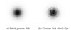 |
Fig. 1 Particle distribution in disk galaxies created with the generator of Springel et al. (2005). After 1 Gyr of isolated evolution spiral structure has developed and star formation self regulated (not shown). |
The initial-condition generator provides a density and velocity distribution of particles. We evolve the created galaxies for 1 Gyr in isolation. In this time, a spiral arm structure forms (see Fig. 1) and 4.8 × 10⁸ M⊙ of stars are produced in the largest galaxy. The radial density structure of our highest mass galaxy is very similar to the one described in S1 (their Fig. 1), but further extended owing to the higher circular velocity in our simulations. After isolated evolution, the galaxies are paired up into binary mergers and, in case of the main runs, inserted into the ICM environment.
2.2. ICM setup
GADGET-2 features only cubical simulation domains with periodic boundaries. For typical galaxy velocities within a cluster (1000 km s-1), this poses a computational problem: to capture at least the first two encounters of a merging pair of galaxies, the domain needs a size of about L = 1 Mpc cubed. To simulate the ICM with GADGET-2, one could fill this domain with gas particles of sufficient mass resolution. To avoid numerical artifacts caused by the SPH scheme, the mass resolution of ICM particles has to match that of the galaxie’s gas (Ott & Schnetter 2003). Accurate simulations of both collisionless dynamics and smoothed particle hydrodynamics require a certain mass resolution. as does the star formation recipe. To fill the whole domain with particles of this mass resolution is computationally too expensive. We adapted the approach in K9 with a layered setup with resolution decreasing toward the outer layers and periodic boundaries.
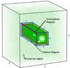 |
Fig. 2 Three-layered ICM setup. Shown is the region of high resolution (inner border, h × h × L) in which the simulated merger takes place, the encompassing sleeve region of lower resolution (border S × S × L) and the rest of the simulation domain (outermost cube of edge length L). The particle’s number density is indicated in shades of green. Galaxies move along the arrow inside the region of high-mass resolution. |
Our setup consists of an inner elongated “windtunnel” of high-resolution particles encompassed by particles with lower resolved masses. These coarser resolved particles keep the inner region stable. To prevent the setup from dissipating, we use periodic boundary conditions. In contrast to K9, our setup introduces an additional layer, a sleeve region around the innermost part, which drops slightly in resolution. This improves stability of the inner region and allows for a steeper resolution drop in the large outer region, thus saving computation time. The setup is shown in Fig. 2. The overall ICM density does not change by more than 2% in the inner region of our simulations. Dissipation and density fluctuations are suppressed better than in K9. The mean distance of particles that have escaped the inner region from the region’s edges is up to 20% less in our setup than with K9, while their number decreases by 30%. Depending on the merger geometry, the “windtunnel” typically has a size of 120 × 120 × 1000 kpc with a sleeve width of 60 kpc1. This gives a time of 1 Gyr for the galaxies to pass through.
The high-resolution region is large enough to hold all of the galaxies’ gas and most of the wake at all times during the merger. The cube size is sufficient for the whole extent of the galaxies’ dark matter halo. It must be noted, however, that the periodic images of the galaxies still contribute to the overall potential. These are in principle unphysical and introduce small force errors. The ICM throughout this work is modeled with a temperature of 107 K, which is consistent with typical ambient gas temperatures in a cluster.
In other ram pressure simulations, S1 and Jáchym et al. (2007, 2009) find little dependence of SFR and stripping fraction on the direction of ICM flow with respect to disk orientation. Nearly edge-on cases (within ≈20°) only had significant deviations in stripping fraction from the cases where galaxies encountered the ICM with their disks oriented face-on to the ICM. However, the differences in SFR were negligible in all cases. Based on these results, and owing to other restrictions discussed in Sect. 2.3, we chose to sample mostly face-on cases, with two edge-on ICM scenarios for completeness. The ICM densities in our simulations range from 10-27 to 10-29 g cm-3. Adopting a standard β model2 for the ICM density, these values correspond to cluster-centric distances of 0.5, 0.8, 1.8, 2.6, and 5.6 Mpc for Coma, putting our standard case at 0.7  . As such they cover typical densities from the outskirts to the regions where ram pressure dominates our simulations. For Virgo our standard case would correspond to a distance of about 1 Mpc from the center and 0.3 Mpc for the highest density in our simulations (Schindler et al. 1999, Fig. 11b).
The strength of ram pressure, as discussed by Gunn & Gott (1972), is given by
 where Pram is the pressure due to the relative movement of galaxies with respect to the ICM at speed vrel. A gas density of the ICM, ρICM = const., is assumed in our simulations. The amount of stripped gas in this approximation is then determined by the radius at equilibrium between ram pressure and restoring gravitational force. A similar estimate for the stripping timescale can be made by comparing acceleration due to ram pressure with restoring acceleration due to gravity.
It was found, e.g., by K9 that SFR has a stronger dependence on ρICM than on vrel. Consequently, we sampled five different ICM densities in contrast to only two speeds within the ICM (see Table 3).
2.3. Merger setup
For the most general case of a binary merger, the centers of mass of the two galaxies approach each other at approximately Keplerian orbits. The angular momenta of their disks with respect to the orbital plane can have arbitrary orientations. The ICM flow may come from an arbitrary direction as well.
However, the treatment of ICM in our simulations limits the range of some of the individual geometric parameters of the merger; that is, we can only simulate those geometries that fit within the high-resolution region of the ICM shown in Fig. 2. For convenience, we align the orbital plane with our “windtunnel”. To capture the whole merging process from the start, the initial separation of both disks, d, must be at least 100 kpc. The number is supported by both our own simulations and observations (Ellison et al. 2010; Li et al. 2008; Lambas et al. 2003). At this distance, gravitational interaction can be neglected for star formation and stripping, and the whole merging process is captured.
Lambas et al. (2003) found significant enhancement in star formation only in galaxies at relative velocities v ≤ 100 km s-1, which is the highest relative initial velocity between two galaxies, which we chose to adapt in our simulations. The effective set of geometrical parameters are illustrated in Fig. 3.
 |
Fig. 3 Geometric merger parameters as used in our simulations. With d, the inital separation, b the inital displacement, as well as β and γ the inclination of the larger and smaller galaxies with respect to the orbital plane. |
 |
Fig. 4 Overall SFR of the reference simulation wstd and its comparison simulations, iμ6 + iμ1 and mμ6. Shown is the added SFR of the single galaxies in ICM and in vacuum (upper and lower dashed lines, respectively), as well as the SFR for the same galaxies merging in vacuum and in an ICM environment (solid lines). The strong peak in vacuum and ICM merger SFRs coincides with the galaxies first encounter at t = 0.4 Gyr. |
3. Results
3.1. Evolution of star formation rate
In this section we investigate the impact of the simulated ram pressure wind on our minor merger’s SFR. Figure 4 shows the evolution of SFR over 1 Gyr of simulation time for our reference case, wstd, and its three comparison runs (non-merging galaxies in vacuum and ICM, merger in vacuum). Similar plots are provided for the most interesting cases simulated. In the plots, we show the total SFR, including stars forming in the ram-pressure-induced wake behind the galaxies, as well as those in the galactic disks. In the next Sect. 3.2, we discuss the distribution of newly formed stars between the two.
In most plots, the SFR shows two distinct peaks at about 25 and 400 Myr into the merger’s evolution. The initial peak in the SFR plots (at ≈25 Myr) should be disregarded. It occurs when the galaxies first encounter the ICM of our setup. In reality they would gradually fall into a cluster’s ICM as opposed to a sudden encounter, when inserted into the “windtunnel” (Sect. 2.2). The disturbance caused by that, however, is overcome after the first 80 Myr of evolution. Simulations including ram pressure show oscillations in their SFR, which can be traced to density fluctuations in the galactic disk. A possible cause is the numerical problem in SPH (see Sect. 3.3), seeing the compressions also occur when the star formation and galactic-wind subgrid model is disabled. The oscillations, however, are not comparable to the physical effects that can be seen in our plots.
In Fig. 4, the second and highest peak at a SFR of 19 M⊙ yr-1 coincides with the time of the galaxies’ first encounter (t ≈ 0.4 Gyr). It is present in both curves that show the merger SFR in the ICM and the vacuum merger’s SFR. As mentioned in the introduction, the origin of these peaks is mostly the triggered gas inflow to the center and higher gas densities due to the disturbance induced by the merging partner.
To put the mergers into perspective, the added vacuum star formation of the individual galaxies involved in the merger (i.e., added SFR of the two separate simulations μ1 and μ6) is also shown in Fig. 4. In a vacuum, the non-merging galaxies form stars at a slowly declining, combined rate of around 3 M⊙ yr-1. The vacuum merger has comparable SFRs up until the first encounter of the merging galaxies at t = 0.4 Gyr and then peaks sharply at 13 M⊙ yr-1. This increase surpasses the combined rate of the individual galaxies in the ICM without a merging partner (sum of SFRs for the simulations labeled “iμ1” and “iμ6”), which is the top curve in Fig. 4. The first encounter peak in the ICM is 25% higher than in the vacuum merger and higher than the non-merging galaxies in ICM. This collaborative effect is a result of the core gas being more compact under ram pressure, making it more susceptible to gas inflows triggered by the merger. The effect, however, is short-lived: the second encounter peak at t ≈ 0.86 Gyr is small in comparison to the vacuum case and barely visible in the ICM merger. By the time of the second encounter, >25% of the gas is stripped, and the gas and stellar disks of both galaxies are severely disturbed by the interaction. These results are consistent with the results of K8. We use more moderate parameters for the galaxies’ gas fraction (15% instead of 25% in K8), resulting in an overall lower SFR compared to K8 and K9. For otherwise comparable galaxies, they have peak values of 26 M⊙ yr-1 at an enhancement in ICM of a factor of 3.5 to 8. The standard case represents the highest relative peak enhancement of SFR in our simulations.
 |
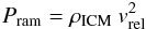
Fig. 5 SFRs for different ICM densities. The higher density run wρ528 in a) shows a minute merger peak and is otherwise indistinguishable from the single galaxies in ICM. Run wρ529 in b), on the other hand, has a visible first encounter peak in ICM that is slightly smaller than in wstd but that still surpasses the peak value in a vacuum. |
The impact of changes in the ICM density is shown in Fig. 5. We omit the plots for wρ27 and wρ29, i.e. highest and lowest simulated ICM densities. They do not differ significantly from their comparison runs for “ram pressure” – only (iμ1ρ27 + iμ6ρ27 in case of wρ27) or vacuum (mμ6) in the case of wρ29 – and thus show a limit for possible collaborative effects.
In both the ICM cases in Fig. 5a (merging and non-merging), overall SFR is steeply declining for ρICM = 5 × 10-28 g cm-3. By the time of the first encounter, when the first SFR peak appears in the vacuum merger, more than 50% of the gas is stripped. Thus, we barely see an enhancement in the ICM merger’s peak SFR over the non-merging galaxies in ICM in Fig. 5a. The vacuum merger peak in SFR at the first encounter in Fig. 5a is below the value for the non-merging galaxies in ICM. In contrast, the lower ram pressure runs, wμ529 and wstd, show a distinct first encounter peak in the ICM merger. Indeed, it is a handy heuristic for the simulations in this work: if any encounter peak in the vacuum merger is at least comparable in height to the overall SFR in ICM single galaxies, the peak can also be seen in the ICM merger.
Varying the relative speed between ICM and the galaxies (wvr500) showed only a decrease in overall star formation by about 15%, when compared to the standard case. Otherwise, wvr500 showed the same peak heights and general behavior as the standard case and is therefore not shown in detail. This behavior is expected, e.g. from K9, because the ICM density is the more crucial parameter for SFR in traditional SPH simulations than is the speed relative to the ICM, although the lower ram pressure via vrel does affect the stripping rate (see Sect. 3.2).
 |
Fig. 6 SFRs for different mass ratios between the merging galaxies. a) Showing wμ4, has a more pronounced second encounter peak in both ICM and vacuum compared to wstd and more even so to wμ8 in b). |
The SFRs for different mass ratios are shown in Fig. 6. Since the partner is more massive and can trigger a stronger starburst, the simulation with mass ratio 1:4 (Fig. 6a) has more pronounced merger peaks in vacuum than the reference case. In the ICM merger, this translates into slightly higher merger peaks as well, but not a proportionate increase. With μ = 1:8 in Fig. 6b, we seem to be at the limit mass ratio for the merger to show any changes in SFR in ICM environments. In the counter-rotating runs, such SFR plots proved to be very similar to their co-rotating counterparts in Fig. 6, with the small increase in SF expected from theory (stemming from additional instability). They were omitted for brevity, but included in the summarizing Fig. 8.
 |
Fig. 7 Simulation wγ90 and related SFRs with inclination angle of the smaller galaxy γ = 90°. The galactic disks are oriented perpendicular to each other, resulting in a longer crossing time and thus broader but flatter vacuum merger peaks. |
Other configurations of angular parameters, i.e., β, γ (see Fig. 3), and the ICM direction are not all shown in distinct plots, but are part of Fig. 8. Variations in these parameters flatten the merger-peaks in vacuum, because the interaction time between the two disk increases or the area for ram pressure to act on is reduced. Different displacements (impact parameters) and initial merger velocities, b and vmer, show little or no merger peaks in the ICM, since the interaction is too short. An example of this general trend is shown in Fig. 7 for γ = 90°. Here the smaller disk feels an edge-on wind, with the larger encountering the ICM face-on. The vacuum merger peaks at around t = 0.4 Gyr and t = 0.85 Gyr are broader compared to wstd but less pronounced. In ICM they are broader as well but barely stand out from the general enhancement due to ram pressure. Of these different geometric configurations, only wb10 has a sharp first encounter peak at 17 M⊙ yr-1 (15 M⊙ yr-1 in the vacuum merger). Just like wstd, the smaller galaxy hits the larger relatively close to its center in a face-on collision and thus yields a comparable outcome.
 |
Fig. 8 Total mass of newly formed stars relative to the added total new star mass of the merger constituents in vacuum. Values are at t = 1 Gyr (end of simulation time). Mergers in the ICM show slightly but not significantly more star mass than the individual galaxies. |
Finally, Fig. 8 shows the relative mass of new stars at the end of the simulations relative to the corresponding mass in the individual galaxies in vacuum. Only one case (wvm75 with lower relative merger velocity) has formed noticeably fewer stars in the ICM merger than its constituent non-merging galaxies in ICM. We attribute this slightly higher SF to stronger perturbations and triggered inflows to the star-forming center due to the merger, as well as the potential wells being deeper (added mass compared to single galaxies). The variance in overall star formation with the individual merger and ICM parameters follows no clear trend and is comparably small. It ranges between almost no difference in the case of γ = 45° to a difference in star mass of 18% between ICM single galaxies and ICM merger in the simulation with edge-on merger and edge-on ICM (wee). The total mass fraction of new stars in the ICM mergers does not follow vacuum merger tendencies; e.g., relative mass of new stars increases slightly from mvm50 to mvm75 (vacuum mergers) but decreases between the ICM case (wvm50, wvm75).
With the exception of a narrow time frame around the first impact of the two merging galaxies, our simulations show negligible contributions of minor mergers to the SFR even in low-density environments (e.g., on the outskirts of typical clusters, outside the virial radius).
3.2. Stripping and star formation in the wake
The time evolution of gas and star-mass fractions in the wake is plotted in Fig. 9 for the reference case wstd. We show these same fractions for the combined masses of the non-merging galaxies as well, in order to provide a comparison. With the star formation recipe used, wake stars form mainly in nodes of stripped gas (see S1, K8). Our criterion for wake stars and gas is simple: we consider particles to be part of the wake, if they lag 40 kpc behind the common center of mass of the stellar disks. This way we can use a uniform criterion across our simulations, thereby covering all the unbound gas. The result of a binding energy-based criterion for identifying wake gas agrees reasonably with this simpler criterion, with a delay of ≈50 Myr.
Initially all curves in Fig. 9 show a fast increase in wake mass fractions. When the gas stripping approaches the equilibrium predicted by Gunn & Gott (1972), the slope becomes shallower. In Fig. 9 this occurs after t ≈ 0.35 Gyr for gas and t ≈ 0.5 Gyr for the stellar component. In principle, the stellar component follows the trend set by the galaxies’ gas with a temporal delay of just over 0.1 Gyr. The increasing offset is a result of the reaccretion of wake stars by the galaxies, because stars no longer feel the ram pressure caused by the relative motion against the ICM. Notable as well is a difference in wake mass of both the stellar and gaseous components, when comparing single and merging galaxies. After the first 0.3 Gyr, the single galaxies experience a higher stripping fraction than in the respective merger scenario. The added mass of the second galaxy in the merger, as well as the fact that the merging partner collects some of the stripped gas after first passage, explains this discrepancy. The additional galaxy increases the potential barrier for gas to escape, once the galaxies are sufficiently close. The companion galaxy overtakes the stripped gas in many of our simulations and binds some of it again.
In our mass regime and predominant merger geometry, this effect compensates for more turbulent gas and tidal features of the merger (such as the bridge), which are more readily stripped. It does, however, depend on the exact merger geometry, as can be seen from wee and wβγ, where re-accreation of gas hardly occurs. Figure 10 shows the same plot for a smaller secondary galaxy. It is comparable to that of Fig. 9 with a slightly higher stripping fraction and higher ratio of star formation in the wake, although it shows a jump in stripping fraction for single galaxies at t ≈ 0.65 Gyr. The cause of this jump is the core of the smaller galaxy finally being stripped. It is only weakly bound until that time. In the ICM merger, the larger galaxy helps retain this core.
 |
Fig. 9 Fraction of stripped gas to total gas mass of the galaxies (upper two lines) and mass of stars newly formed in the wake relative to the total mass of new stars (lower two lines). Shown are the values for both the merger (solid lines) and the added single galaxies (dotted lines) in ICM for wstd. |
 |
Fig. 10 Stripping fraction at a merger mass ratio of μ = 1:8. The curves shown here for the simulations wμ8 in Table 3 are quantitatively the same as in Fig. 9 with slightly more gas being stripped. |
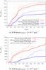 |
Fig. 11 Stripping fractions for the different ICM densities of the simulations wρ528 and wρ529. Note the different scales on the ordinate. The case for lower density b) does not reach its saturation point within the simulation time of 1 Gyr and has a later onset in the wake star fraction. |
Figure 11 shows the situation at higher density (Fig. 11a) and lower density (Fig. 11b). In case of higher density (Fig. 11a), the stripping rate is enhanced by about a factor of three compared to wstd. About 40% of stars are located in the wake by the time saturation is reached in the higher density ICM. The relative difference between the curves for single and merging galaxies becomes smaller at higher densities. At higher densities, the stripping is faster and more severe, giving the merger less time to influence the process. Clearly, ram pressure is the dominant effect here.
At lower densities (Fig. 11b), gas stripping is a more continuous process, with no clear saturation phase. The instability caused by the merger enables gas to be stripped even at later times, when the single galaxies would have reached their saturation point. In the merger, however, gas stripped at later times forms fewer stars than do single galaxies. The disturbance in the gas disk is much greater then, allowing for less star-forming nodes in the wake. At even lower densities (simulation wρ29; plot omitted), only 5% of gas is stripped by the end of the simulation time with less than 1% of all newly formed stars in the wake.
 |
Fig. 12 Stripping fraction for a lower relative velocity of vr = 500 km s-1 than in wstd of Fig. 9. The plot shows that significantly less mass is being stripped, and stars are noticeably re-accreted toward the end of simulation. |
In the graph of Fig. 12, where the stripping fractions of the runs with relative velocity of vr = 500 kms-1 are shown, we see drastically decreased stripping and even less star mass in the wake. Contrary to the situation for overall SFR in the previous section, a lower velocity relative to the ICM has a strong influence on the location of star formation (wake vs. disk). Toward the end of the simulation in Fig. 12, after t = 0.75 Gyr, even re-accretion of stars is visible, as the lower solid curve declines slightly. This is the only simulation to show a decrease in the wake’s stellar mass fraction.
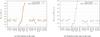 |
Fig. 13 Gas and new star mass in the wake relative to the respective components’ total mass (t = 1 Gyr). Shown are the values for both the merger simulations in ICM and the added single galaxies in ICM that make up the respective merger. |
Figure 13 concludes this section by summarizing the results of all simulations. In Fig. 13a one can see the amount of gas in the wake, again relative to the respective galaxies’ total gas mass. Shown are only the values at the end of the simulation. Geometric merger parameters show little effect on the amount of gaseous material in the wake between merging and non-merging galaxies. Compared to the single galaxies in ICM, slightly less material gets stripped in the scenarios involving a minor merger, though this is dependent on merger geometry. The difference in stripped mass fraction between merging and non-merging galaxies in our simulations ranges from almost none (wβγ) up to 25%; for example, wμ8 has 26% of its gas residing in the wake, while its constituent galaxies iμ8 and iμ1 combined have 33%.
Figure 13b shows the same situation for the fraction of new stellar mass in the wake to total new stellar mass by the end of the simulations. Overall, the fraction of new stars formed in the wake is lower in the merger simulations compared to the single galaxies. As little as half the fractional new stellar content in the wake of single galaxies can be seen in the wake of the respective merger cases. This is to some extent a result of the added mass in the mergers. More so, in most of our simulations the merging partner comes close to the wake of the other galaxy. That enables the partner to accrete some of the stars from the wake of the other galaxy. In the runs where the merging partner does not approach the wake (wee and wmβγ) closely, the differences are smaller. At higher densities, stripping is mostly complete before merger effects start to contribute. At lower densities, ram pressure stripping is no longer a factor, and the difference between merging and non-merging galaxies is small. Only intermediate densities and favorable trajectories of the merging partner lead to collaborative effects. In the light of our simulations, taking minor mergers into account in the process of ram pressure stripping does not yield significantly different results from ram-pressure-only scenarios (except for the wake’s stellar content in the mentioned circumstances).
3.3. Discussion and related work
Unlike our simulations of constant ram pressure, real cluster galaxies experience varying ρICM, depending on their path within the cluster. The recent study of Bekki (2014) uses a β-profile for ρICM and model ram pressure along different galaxy paths with an SPH code to quantify the effect of varying density on SFRs. Their “MW-type” galaxy model is similar to the larger merging partner in our simulations with less total mass (1012 M⊙). Their “M33” is most similar to our iμ8. The Virgo and group-like ICM models in Bekki (2014) yield a SFR enhancement by a factor of 2−3 (compared to our 3−5 × enhancement), but only in the Gyr after the pericenter passage of the galaxies and very shortly before. At this time in the galaxies’ orbits within the Virgo model, ICM density would be >5 × 10-28 g cm-3. This is different behavior from our individual galaxies in ICM that reach their enhancement sooner, after only 0.2 Gyr and generally show stronger enhancement.
A physical explanation may be that gradual infall removes gas gently without causing the conditions that increase SFR in our simulations. With star-forming gas then missing at later times, enhancement in SFR at higher density might not be as drastic until the short-term peak density at pericenter passage comes into play. It is difficult, though, to separate the physical effects from the different numerical models for star formation used in both our studies and other details of the simulation. Jáchym et al. (2007, 2009) studied stripping rates using the same approach for varying ρICM as Bekki (2014). Their results indicate that short time variations in ram pressure do not affect the stripping rate. Instead, the total encountered column density of ICM is the crucial parameter for the amount of material stripped.
We identified the deeper potential well and re-accretion by the merging partner’s increased reach to be the cause of less pronounced gas stripping and fewer stars in the wake of galaxies merging in the ICM. We expect qualitatively similar stripping fractions under variable ram pressure. When compared to simulations with adaptive mesh refinement (AMR), our simulations, and SPH simulations in general, differ greatly in SFR. AMR simulations consistently show quenching rather than an increase in SFR under ram pressure. Tonnesen & Bryan (2012) compare the approach of K9 to their AMR simulations and to observations. They attribute SPH problems with resolving fluid instabilities and the resulting under-mixing, as well as the stiff equation of state as a cause for a high SFR in the tail. These and related problems with the standard pressure-entropy formulation of SPH have been discussed in Agertz et al. (2007) and Hopkins (2013). The problems are most notable in the stripped tail, where much of the star formation takes place in dense nodes of gas. This leads to increased stability and higher density of the star-forming nodes in the wake. Generally in GADGET-2’s formulation of SPH, strong density discontinuities lead to a false pressure estimate (which relies on a smooth density gradient), resulting in an unphysical separation force. Heß & Springel (2012) showed that a gap between ICM and ISM can form because of that, which could cause the density oscillations in the disk. This also keeps disk particles in the star-forming regime, especially at later times, when fluid instabilities and mixing would decrease star formation. Observations support lower SFRs than in our simulations (Boissier et al. 2012).
Vollmer et al. (2012) finds possible enhancement factors of 1.5−2 on the windward side of his sample galaxies in Virgo, while the overall effect is suppression of star formation, especially in the tail. Star-forming tails were found, among others, by Sun et al. (2007) and more recently Ebeling et al. (2014). The former estimates the total mass of current star bursts in the tail’s nodes to be several 107 M⊙, asserting the total stellar mass formed in the tail could be a few times higher from already faded nodes. Ebeling et al. (2014) shows strong galactic starbursts that are likely to be very short in duration. Hester et al. (2010) investigated the Virgo dwarf galaxy IC 3418, finding nodes of dense gas, generally rare in other Virgo galaxies, which Jáchym et al. (2013) studied in greater detail. The total stellar mass in the tail of IC3418, however, is less than 1% of the galaxies stellar mass with tail SFRs of ~0.002 M⊙ yr-1. Heß & Springel (2012) compared the behavior of galaxies in a windtunnel between GADGET-2 and the moving mesh code AREPO (Springel 2010). They demonstrated an overestimation by a factor of two in SFR and a smaller stripping fraction in SPH.
Our objective with this paper has been to determine whether minor mergers have an effect on stripping and SF that should be considered. Although the issues discussed with SPH pose conceptional problems, we use relative quantities and compare, for instance, the relative increase in stripping fraction or SF between merging and non-merging galaxies in the ICM. Moreover, our conclusion is that the effects of merging in the ICM are not significantly different from regular ram-pressure effects on single galaxies.
Hayward et al. (2014) found that pure merger simulations using the standard density-entropy formulation of SPH compare well with results from state-of-the-art, grid-based hydrodynamic codes (i.e., AREPO). The physical processes that could conceivably have led to synergies of ram pressure and merging (gas inflow to the Galactic center, shocks, and disturbance of the gaseous disk from the merger, augmented by increased pressure from the ICM) are accurately modeled in the case of pure mergers or overestimated in SPH or while the counteracting stripping and mixing of the gas phases is underestimated. Therefore the, in any case, small collaborative effects should be even less distinct in these codes, and our conclusion should hold.
4. Conclusions
We have presented GADGET-2 simulations of merging galaxies in the ICM and compared them to galaxies evolved without a merger partner. Our simulations involved gas-rich spiral type galaxies in minor mergers (mass ratios between 1:4 and 1:8) and included their first two encounters.
In general, the merging galaxies retain 5% to 10% more gas in their disk than do galaxies without a merger partner; i.e., less of their gas is located in the ram-pressure stripped wake. The added mass of the merging parter and re-accretion of wake gas by the partner (depending on trajectory) compensate for the disturbance of the gas disk that should make stripping easier. Owing to re-accretion of stars and the added gravitational potential of the merging partners, we typically found 50% fewer stars in the wake of merging galaxies. This effect depends strongly on the trajectory of the galaxies with respect to the wind direction. The relative differences are smaller in simulations with higher ICM density as ram pressure begins to dominate.
Even on the outskirts of clusters, with typical densities of ρICM = 10-28 g cm-3, our simulations indicate little overall effects on SFR owing to ongoing merging activity. We observe a short-term enhancement in SFR, compared to the merger in vacuum of up to 50%, but typically only 20%. These enhancements occur at the time of the first fly-through, when ram pressure condensed the core gas, making it more susceptible to SF induced by the merging partner. Second encounters rarely show any SFR peaks in most cases. Where they do, the enhancements are not higher than 20% over the added SFR of the individual galaxies in ICM. By the time of the second encounter, the galaxies’ disks are too disturbed, and too much gas is stripped. In any case the short-term enhancements do not last longer than 50 Myr and do not contribute much to the overall star mass. When comparing the new star mass formed by the end of our simulations, generally the merging galaxies have formed slightly more stars, typically around 5% but up to 18% more than the individual constituent galaxies in ICM after a time of 1 Gyr. Depending mostly on ICM density and geometric parameters, the reason for this higher star formation in our simulations is a denser core and gas inflow triggered by the merging partner. We discussed possible issues in Sect. 3.3. They boil down to unphysical pressure estimates at the interface between ICM and ISM, possibly leading to an overestimation of the collaborative effects. For overall star formation, the effect of varying geometric and ICM parameters related to ram pressure stripping dominates those of the minor merger parameters (mass ratio, merger geometry), and collaborative effects are small in any case.
Corresponds to h × h × L in Fig. 2. Sleeve width:  kpc.
kpc.
β-Model of Cavaliere & Fusco-Femiano (1978): ρICM(r) = ρ0 [ 1 + (r/rc)2 ] −3/2β. Parameters for the Coma cluster (Mohr et al. 1999) are: β = 0.7, rc = 0.26 Mpc and ρ0 = 6.3 × 10⁻²⁷ g cm-3.
Acknowledgments
The authors thank the anonymous referee, who helped to improve the quality of the paper significantly. The authors acknowledge the UniInfrastrukturprogramm des BMWF Forschungsprojekt Konsortium Hochleistungsrechnen and the doctoral school – Computational Interdisciplinary Modelling FWF DK-plus (W1227). D.S. acknowledges the research grant from the office of the vice rector for research of the University of Innsbruck (project DB: 194272). The authors thank Volker Springel for providing the simulation code GADGET-2 and the initial-conditions generator. We furthermore acknowledge profitable discussions with the colleagues at the institute.
References
- Abadi, M. G., Moore, B., & Bower, R. G. 1999, MNRAS, 308, 947 [NASA ADS] [CrossRef] [Google Scholar]
- Agertz, O., Moore, B., Stadel, J., et al. 2007, MNRAS, 380, 963 [NASA ADS] [CrossRef] [Google Scholar]
- Barnes, J., & Hut, P. 1986, Nature, 324, 446 [NASA ADS] [CrossRef] [Google Scholar]
- Bekki, K. 2014, MNRAS, 438, 444 [NASA ADS] [CrossRef] [Google Scholar]
- Berrier, J. C., Stewart, K. R., Bullock, J. S., et al. 2009, ApJ, 690, 1292 [NASA ADS] [CrossRef] [Google Scholar]
- Boissier, S., Boselli, A., Duc, P.-A., et al. 2012, A&A, 545, A142 [NASA ADS] [CrossRef] [EDP Sciences] [Google Scholar]
- Bournaud, F., Elmegreen, B. G., Teyssier, R., Block, D. L., & Puerari, I. 2010, MNRAS, 409, 1088 [NASA ADS] [CrossRef] [Google Scholar]
- Butcher, H., & Oemler, Jr., A. 1978, ApJ, 219, 18 [NASA ADS] [CrossRef] [Google Scholar]
- Butcher, H., & Oemler, Jr., A. 1984, ApJ, 285, 426 [NASA ADS] [CrossRef] [Google Scholar]
- Cavaliere, A., & Fusco-Femiano, R. 1978, A&A, 70, 677 [NASA ADS] [Google Scholar]
- Cayatte, V., van Gorkom, J. H., Balkowski, C., & Kotanyi, C. 1990, AJ, 100, 604 [NASA ADS] [CrossRef] [Google Scholar]
- De Lucia, G., Weinmann, S., Poggianti, B. M., Aragón-Salamanca, A., & Zaritsky, D. 2012, MNRAS, 423, 1277 [NASA ADS] [CrossRef] [Google Scholar]
- Ebeling, H., Stephenson, L. N., & Edge, A. C. 2014, ApJ, 781, L40 [NASA ADS] [CrossRef] [Google Scholar]
- Elbaz, D., & Cesarsky, C. J. 2003, Science, 300, 270 [NASA ADS] [CrossRef] [PubMed] [Google Scholar]
- Ellison, S. L., Patton, D. R., Simard, L., et al. 2010, MNRAS, 407, 1514 [NASA ADS] [CrossRef] [Google Scholar]
- Elmegreen, B. G. 2011, in EAS Pub. Ser. 51, eds. C. Charbonnel, & T. Montmerle, 3 [Google Scholar]
- Farouki, R., & Shapiro, S. L. 1980, ApJ, 241, 928 [NASA ADS] [CrossRef] [Google Scholar]
- Gingold, R. A., & Monaghan, J. J. 1977, MNRAS, 181, 375 [Google Scholar]
- Gnedin, O. Y. 2003, ApJ, 582, 141 [NASA ADS] [CrossRef] [Google Scholar]
- Gunn, J. E., & Gott, III, J. R. 1972, ApJ, 176, 1 [NASA ADS] [CrossRef] [Google Scholar]
- Hayward, C. C., Torrey, P., Springel, V., Hernquist, L., & Vogelsberger, M. 2014, MNRAS, 442, 1992 [NASA ADS] [CrossRef] [Google Scholar]
- Hernquist, L. 1990, ApJ, 356, 359 [NASA ADS] [CrossRef] [Google Scholar]
- Heß, S., & Springel, V. 2012, MNRAS, 426, 3112 [NASA ADS] [CrossRef] [Google Scholar]
- Hester, J. A., Seibert, M., Neill, J. D., et al. 2010, ApJ, 716, L14 [NASA ADS] [CrossRef] [Google Scholar]
- Hopkins, P. F. 2013, MNRAS, 428, 2840 [NASA ADS] [CrossRef] [Google Scholar]
- Hopkins, P. F., Quataert, E., & Murray, N. 2011, MNRAS, 417, 950 [NASA ADS] [CrossRef] [Google Scholar]
- Irwin, J. A., Seaquist, E. R., Taylor, A. R., & Duric, N. 1987, ApJ, 313, L91 [NASA ADS] [CrossRef] [Google Scholar]
- Jáchym, P., Palouš, J., Köppen, J., & Combes, F. 2007, A&A, 472, 5 [NASA ADS] [CrossRef] [EDP Sciences] [Google Scholar]
- Jáchym, P., Köppen, J., Palouš, J., & Combes, F. 2009, A&A, 500, 693 [NASA ADS] [CrossRef] [EDP Sciences] [Google Scholar]
- Jáchym, P., Kenney, J. D. P., Ržuička, A., et al. 2013, A&A, 556, A99 [NASA ADS] [CrossRef] [EDP Sciences] [Google Scholar]
- Joseph, R. D., Meikle, W. P. S., Robertson, N. A., & Wright, G. S. 1984, MNRAS, 209, 111 [Google Scholar]
- Kapferer, W., Knapp, A., Schindler, S., Kimeswenger, S., & van Kampen, E. 2005, A&A, 438, 87 [NASA ADS] [CrossRef] [EDP Sciences] [Google Scholar]
- Kapferer, W., Kronberger, T., Ferrari, C., Riser, T., & Schindler, S. 2008, MNRAS, 389, 1405 [NASA ADS] [CrossRef] [Google Scholar]
- Kapferer, W., Sluka, C., Schindler, S., Ferrari, C., & Ziegler, B. 2009, A&A, 499, 87 [NASA ADS] [CrossRef] [EDP Sciences] [Google Scholar]
- Katz, N., Weinberg, D. H., & Hernquist, L. 1996, ApJS, 105, 19 [NASA ADS] [CrossRef] [Google Scholar]
- Kennicutt, Jr., R. C. 1998, ApJ, 498, 541 [NASA ADS] [CrossRef] [Google Scholar]
- Kronberger, T., Kapferer, W., Schindler, S., et al. 2006, A&A, 458, 69 [NASA ADS] [CrossRef] [EDP Sciences] [Google Scholar]
- Kronberger, T., Kapferer, W., Ferrari, C., Unterguggenberger, S., & Schindler, S. 2008, A&A, 481, 337 [NASA ADS] [CrossRef] [EDP Sciences] [Google Scholar]
- Lackner, C. N., & Gunn, J. E. 2013, MNRAS, 428, 2141 [NASA ADS] [CrossRef] [Google Scholar]
- Lambas, D. G., Tissera, P. B., Alonso, M. S., & Coldwell, G. 2003, MNRAS, 346, 1189 [NASA ADS] [CrossRef] [Google Scholar]
- Li, C., Kauffmann, G., Heckman, T. M., Jing, Y. P., & White, S. D. M. 2008, MNRAS, 385, 1903 [NASA ADS] [CrossRef] [Google Scholar]
- Lucy, L. B. 1977, AJ, 82, 1013 [NASA ADS] [CrossRef] [Google Scholar]
- McGee, S. L., Balogh, M. L., Bower, R. G., Font, A. S., & McCarthy, I. G. 2009, MNRAS, 400, 937 [NASA ADS] [CrossRef] [Google Scholar]
- Mihos, C. 2003 [arXiv:astro-ph/0305512] [Google Scholar]
- Mo, H. J., Mao, S., & White, S. D. M. 1998, MNRAS, 295, 319 [Google Scholar]
- Mohr, J. J., Mathiesen, B., & Evrard, A. E. 1999, ApJ, 517, 627 [NASA ADS] [CrossRef] [Google Scholar]
- Navarro, J. F., Frenk, C. S., & White, S. D. M. 1996, ApJ, 462, 563 [NASA ADS] [CrossRef] [Google Scholar]
- Noguchi, M. 1988, A&A, 203, 259 [NASA ADS] [Google Scholar]
- Ostriker, J. P. 1980, Comments on Astrophysics, 8, 177 [Google Scholar]
- Ott, F., & Schnetter, E. 2003 [arXiv:physics/0303112] [Google Scholar]
- Roediger, E., & Brüggen, M. 2006, MNRAS, 369, 567 [NASA ADS] [CrossRef] [Google Scholar]
- Roediger, E., & Brüggen, M. 2007, MNRAS, 380, 1399 [NASA ADS] [CrossRef] [Google Scholar]
- Roediger, E., Brüggen, M., Owers, M. S., Ebeling, H., & Sun, M. 2014, MNRAS, 443, L114 [NASA ADS] [CrossRef] [Google Scholar]
- Schindler, S., Binggeli, B., & Böhringer, H. 1999, A&A, 343, 420 [NASA ADS] [Google Scholar]
- Schmidt, M. 1959, ApJ, 129, 243 [NASA ADS] [CrossRef] [Google Scholar]
- Schulz, S., & Struck, C. 2001, MNRAS, 328, 185 [NASA ADS] [CrossRef] [Google Scholar]
- Springel, V. 2005, MNRAS, 364, 1105 [NASA ADS] [CrossRef] [Google Scholar]
- Springel, V. 2010, MNRAS, 401, 791 [NASA ADS] [CrossRef] [Google Scholar]
- Springel, V., & Hernquist, L. 2002, MNRAS, 333, 649 [NASA ADS] [CrossRef] [Google Scholar]
- Springel, V., & Hernquist, L. 2003, MNRAS, 339, 289 [Google Scholar]
- Springel, V., Di Matteo, T., & Hernquist, L. 2005, MNRAS, 361, 776 [NASA ADS] [CrossRef] [Google Scholar]
- Steinhauser, D., Haider, M., Kapferer, W., & Schindler, S. 2012, A&A, 544, A54 [NASA ADS] [CrossRef] [EDP Sciences] [Google Scholar]
- Sun, M., Donahue, M., & Voit, G. M. 2007, ApJ, 671, 190 [NASA ADS] [CrossRef] [Google Scholar]
- Tonnesen, S., & Bryan, G. L. 2012, MNRAS, 422, 1609 [NASA ADS] [CrossRef] [Google Scholar]
- Toomre, A., & Toomre, J. 1972, ApJ, 178, 623 [NASA ADS] [CrossRef] [Google Scholar]
- Vollmer, B., Cayatte, V., Balkowski, C., & Duschl, W. J. 2001, ApJ, 561, 708 [NASA ADS] [CrossRef] [Google Scholar]
- Vollmer, B., Wong, O. I., Braine, J., Chung, A., & Kenney, J. D. P. 2012, A&A, 543, A33 [NASA ADS] [CrossRef] [EDP Sciences] [Google Scholar]
- Xu, G. 1995, ApJS, 98, 355 [NASA ADS] [CrossRef] [Google Scholar]
All Tables
Important parameters used in all simulations (see Springel & Hernquist 2003; Springel 2005).
All Figures
|
Fig. 1 Particle distribution in disk galaxies created with the generator of Springel et al. (2005). After 1 Gyr of isolated evolution spiral structure has developed and star formation self regulated (not shown). |
| In the text | |
|
Fig. 2 Three-layered ICM setup. Shown is the region of high resolution (inner border, h × h × L) in which the simulated merger takes place, the encompassing sleeve region of lower resolution (border S × S × L) and the rest of the simulation domain (outermost cube of edge length L). The particle’s number density is indicated in shades of green. Galaxies move along the arrow inside the region of high-mass resolution. |
| In the text | |
|
Fig. 3 Geometric merger parameters as used in our simulations. With d, the inital separation, b the inital displacement, as well as β and γ the inclination of the larger and smaller galaxies with respect to the orbital plane. |
| In the text | |
|
Fig. 4 Overall SFR of the reference simulation wstd and its comparison simulations, iμ6 + iμ1 and mμ6. Shown is the added SFR of the single galaxies in ICM and in vacuum (upper and lower dashed lines, respectively), as well as the SFR for the same galaxies merging in vacuum and in an ICM environment (solid lines). The strong peak in vacuum and ICM merger SFRs coincides with the galaxies first encounter at t = 0.4 Gyr. |
| In the text | |
|
Fig. 5 SFRs for different ICM densities. The higher density run wρ528 in a) shows a minute merger peak and is otherwise indistinguishable from the single galaxies in ICM. Run wρ529 in b), on the other hand, has a visible first encounter peak in ICM that is slightly smaller than in wstd but that still surpasses the peak value in a vacuum. |
| In the text | |
|
Fig. 6 SFRs for different mass ratios between the merging galaxies. a) Showing wμ4, has a more pronounced second encounter peak in both ICM and vacuum compared to wstd and more even so to wμ8 in b). |
| In the text | |
|
Fig. 7 Simulation wγ90 and related SFRs with inclination angle of the smaller galaxy γ = 90°. The galactic disks are oriented perpendicular to each other, resulting in a longer crossing time and thus broader but flatter vacuum merger peaks. |
| In the text | |
|
Fig. 8 Total mass of newly formed stars relative to the added total new star mass of the merger constituents in vacuum. Values are at t = 1 Gyr (end of simulation time). Mergers in the ICM show slightly but not significantly more star mass than the individual galaxies. |
| In the text | |
|
Fig. 9 Fraction of stripped gas to total gas mass of the galaxies (upper two lines) and mass of stars newly formed in the wake relative to the total mass of new stars (lower two lines). Shown are the values for both the merger (solid lines) and the added single galaxies (dotted lines) in ICM for wstd. |
| In the text | |
|
Fig. 10 Stripping fraction at a merger mass ratio of μ = 1:8. The curves shown here for the simulations wμ8 in Table 3 are quantitatively the same as in Fig. 9 with slightly more gas being stripped. |
| In the text | |
|
Fig. 11 Stripping fractions for the different ICM densities of the simulations wρ528 and wρ529. Note the different scales on the ordinate. The case for lower density b) does not reach its saturation point within the simulation time of 1 Gyr and has a later onset in the wake star fraction. |
| In the text | |
|
Fig. 12 Stripping fraction for a lower relative velocity of vr = 500 km s-1 than in wstd of Fig. 9. The plot shows that significantly less mass is being stripped, and stars are noticeably re-accreted toward the end of simulation. |
| In the text | |
|
Fig. 13 Gas and new star mass in the wake relative to the respective components’ total mass (t = 1 Gyr). Shown are the values for both the merger simulations in ICM and the added single galaxies in ICM that make up the respective merger. |
| In the text | |
Current usage metrics show cumulative count of Article Views (full-text article views including HTML views, PDF and ePub downloads, according to the available data) and Abstracts Views on Vision4Press platform.
Data correspond to usage on the plateform after 2015. The current usage metrics is available 48-96 hours after online publication and is updated daily on week days.
Initial download of the metrics may take a while.