| Issue |
A&A
Volume 575, March 2015
|
|
|---|---|---|
| Article Number | L16 | |
| Number of page(s) | 4 | |
| Section | Letters | |
| DOI | https://doi.org/10.1051/0004-6361/201525627 | |
| Published online | 10 March 2015 | |
High-redshift active galactic nuclei and H I reionisation: limits from the unresolved X-ray background
1 DiSAT, Università dell’Insubria, via Valleggio 11, 22100 Como, Italy
e-mail: haardt@mib.infn.it
2 INFN, Sezione di Milano-Bicocca, Piazza delle Scienze 3, 20123 Milano, Italy
3 INAF, IASF Milano, via E. Bassini 15, 20133 Milano, Italy
Received: 8 January 2015
Accepted: 10 February 2015
The rapidly declining population of bright quasars at z ≳ 3 appears to make an increasingly smaller contribution to the ionising background at the H I Lyman limit. It is thererfore generally thought that massive stars in (pre-)Galactic systems may provide the additional ionising flux needed to complete H I reionisation by z ≳ 6. A galaxy-dominated background, however, may require that the escape fraction of Lyman continuum radiation from high-redshift galaxies is as high as 10%, which is somewhat at odds with (admittedly scarce) observational constraints. High escape fractions from dwarf galaxies have been advocated, or, alternatively, a so-far undetected (or barely detected) population of unobscured, high-redshift faint AGNs. Here we examine the latter hypothesis and show that such sources, to be consistent with the measured level of the unresolved X-ray background at z = 0, can provide a fraction of the H II filling factor no larger than 13% by z ≃ 6. The fraction rises to ≲27% in the somewhat extreme case of a constant comoving redshift evolution of the AGN emissivity. This still calls for a mean escape fraction of ionising photons from high-z galaxies of ≳10%.
Key words: cosmology: observations / X-rays: diffuse background / galaxies: active
© ESO, 2015
1. Introduction
The reionisation of the all-pervading intergalactic medium (IGM) is a landmark event in the history of the Universe. Studies of the so-called Gunn-Peterson absorption in the spectra of distant quasars show that hydrogen was already highly ionised out to redshift z ~ 6 (e.g., Songaila 2004; Fan et al. 2006), while cosmic microwave background polarisation data constrain the redshift of a sudden reionisation event to be significantly higher, z ~ 10 (Jarosik et al. 2011; Hinshaw et al. 2013). Most of our understanding of IGM physics, and its implication for galaxy formation and metal enrichment, critically depends on the properties of the cosmic ionising background. While it is generally thought that the gas is kept ionised by the integrated UV emission from active galactic nuclei (AGNs) and star-forming galaxies (Miralda-Escude & Ostriker 1990; Haardt & Madau 1996), the relative contributions of these sources as a function of cosmic time are poorly known.
At z ≳ 3, the declining population of bright quasars appears to make an increasingly smaller contribution to the ionising radiation background at the H I Lyman limit. It was therefore suggested that massive stars in Galactic systems may provide the additional ionising flux needed at early times (e.g., Madau et al. 1999; Gnedin 2000; Wyithe & Loeb 2003; Meiksin 2005; Trac & Cen 2007; Faucher-Giguère et al. 2008; Gilmore et al. 2009; Robertson et al. 2010). However, leaking Lyman continuum radiation from bright galaxies seems to be modest (see, e.g., Vanzella et al. 2010), and it has therefore been argued that dwarf galaxies (with a virial mass below ~109M⊙) may produce the dominant contribution to the H I ionising UV background (e.g., Robertson & Ellis 2012).
Alternative to invoking a major contribution to reionisation from dwarf(ish) galaxies is the possibility that the AGN emissivity at z ≳ 4 is indeed much higher than generally thought. Indications along such line have been reported by several groups (Glikman et al. 2011; Civano et al. 2011; Fiore et al. 2012), although it is fair to say that results seem not univocal (see, e.g., Masters et al. 2012). Very recently, Giallongo et al. (2015) found 22 AGN candidates at z ≳ 4 in the Candel/GOOD-S/Chandra Deep Field South field, which is suggestive of a prominent contribution of AGNs to the ionising background in the range 4 ≲ z ≲ 6.5. The resulting H I photoionisation rate is indeed consistent with various estimates at the same redshifts, based on both the flux-decrement and proximity-effect techniques (Becker et al. 2007; Calverley et al. 2011).
The high-redshift population of AGNs should leave an imprint in the observed cosmic X-ray background (XRB). Chandra deep observations resolved the XRB into discrete sources at a level of 80–90% over the entire bandwidth (0.5–2 keV), with only a fraction ~1% of the signal arising from sources located at z ≳ 4 (Xue et al. 2011). Moretti et al. (2012) exploited the very low instrumental noise of the Swift XRT to measure the still unresolved XRB spectrum at the highest accuracy. Salvaterra et al. (2012) used such measures to place upper limits on the cosmic accretion history of massive black holes. An obvious caveat to our conclusions is the possible existence of a large population of severely obscured (log NH ≳ 25) accreting black holes that do not glow in the X-rays. Unless one were to advocate a very peculiar UV-to-X-ray spectral energy distribution, this caveat would not apply if the unresolved AGN population does contribute significantly to the ionisation background. Assessing the contribution to the XRB of such UV-emitting AGNs is precisely the goal of this Letter. Specifically, we translate the Moretti et al. (2012) upper limits to the unresolved XRB into upper limits on the possible contribution of high-redshift, unobscured faint AGNs to H I reionisation. A similar analysis was proposed by Dijkstra et al. (2004), Salvaterra et al. (2005, 2007), and McQuinn (2012), with conflicting results. Here we use the most updated limits on the XRB and adopt a (h,Ωm,ΩΛ) = (0.7,0.3,0.7) cosmology.
2. Methodology
Assuming an AGN comoving X-ray specific emissivity ∝E− αx(1 + z)− γ, the XRB at observed energy E0 due to sources located at redshift z ≥ zx is 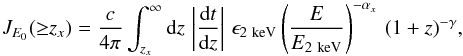 (1)where E = E0(1 + z). We now relate the specific emissivity at 2 keV, ϵ2 keV, to that at 912 Å, that is, ϵ2 keV = Kϵ912 Å, where the K-correction normalisation reads
 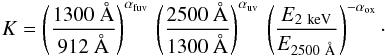 (2)Here αox is the optical-to-X-ray spectral index, defined from the specific emissivity at 2 keV and at 2500 Å, αox ≡ − 0.384log (ϵ2 keV/ϵ2500 Å). In writing Eq. (2), we followed the piece-wise UV AGN spectral energy distribution as described in Haardt & Madau (2012). Now the r.h.s. integral in Eq. (1) is easily solved, and the obtained JE0( ≥ zx) constrained to be no larger than the observational upper limit
  . This in turn gives the highest value of ϵ912 Å consistent with the limits on the unresolved XRB:
 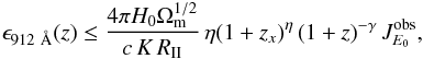 (3)where we neglected the energy density of the cosmological constant (we are interested in the redshift regime z ≫ zmΛ ≃ 0.33). We set η ≡ (γ + αx + 3 / 2), and the term RII ≥ 1 is meant to account for the contribution of obscured AGNs at z ≥ zX to the XRB observed at energy E0.
It is now straightforward to translate this limit into a limit on reionisation. The volume-filling factor of H II regions QHII is the solution of the following differential equation (see Madau et al. 1999): 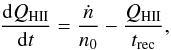 (4)where n0 is the cosmic hydrogen mean density, and ṅ(z) = ϵ912 Å(z) / (hpαfuv) the photon emission rate (hp is the Planck constant, and the FUV emissivity is ∝ν− αfuv). The H II recombination time trec is computed as in Haardt & Madau (2012).
3. Observational parameters
The upper limits given by Eqs. (3) and (4) depend upon a number of parameters that need to be observationally constrained. In this section we discuss the choice we made for each of them.
Unresolved XRB. The unresolved XRB shows a very hard spectrum, suggesting that most (if not all) of the flux comes from low-z obscured AGNs. Indeed, Moretti et al. (2012), by adopting the XRB synthesis model of Gilli et al. (2007), derived a stringent limit  erg cm-2 s-1 Hz-1 sr-1 at E0 = 1.5 keV after accounting for absorbed AGNs at z ≲ 5 whose fluxes lie below the Chandra limit. The synthesis model falls short at E0 ≳ 3 keV, however, suggesting the possible existence of a population of Compton-thick AGNs at intermediate redshifts.
UV and X-ray spectral indices. As already stated, we used the very same parametrisation as Haardt & Madau (2012), adopting for the UV slope αuv = 0.44 (λ> 1300 Å, Vanden Berk et al. 2001), and αfuv = 1.57 in the FUV range (λ< 1300 Å, Telfer et al. 2002). We note for the X-ray spectrum that most of the contribution to the XRB at E0 = 1.5 keV is expected from sources located just above z ≃ 5, that is, from photons emitted at rest-frame energy ≃10 keV. In this energy range unobscured AGNs exhibit a power-law spectrum with index αx ≃ 0.8, as a combination of the intrinsic continuum and of the Compton reflection bump (see, e.g., Ueda et al. 2014). In our analysis we then take αx = 0.8. From Eq. (2) it is apparent that the exact values of the UV and X-ray spectral indices will affect our conclusions only marginally.
Optical-to-X-ray spectral index. The value of αox has a strong effect on our estimate of QHII since (E2 keV/E2500 Å) ≃ 403. The study of the correlation between X-ray and UV luminosities has been the subject of many works on both optically selected and X-ray selected AGNs. Among others, Steffen et al. (2006) found a significant correlation between αox and the monochromatic luminosities at 2500 Å (i.e.,  , with β> 1) in a sample of 333 optically selected AGNs. No significant correlation of αox with redshift was reported. Lusso et al. (2010) analysed a sample of 545 X-ray selected type I AGNs from the XMM-COSMOS survey, finding again a correlation between αox and L2500 Å. The mean value of αox for the full sample was 1.37 with a dispersion around the mean of 0.18. Marchese et al. (2012) also reported a highly significant correlation between αox and the UV luminosity in a sample of 195 X-ray selected type I bright AGNs, basically confirming the results of Lusso et al. (2010). In our investigation the supposedly unaccounted for population of AGNs that is responsible for the H I reionisation must necessarily reside in the very faint end of the UV luminosity function. According to the literature cited above, this would imply a value of αox on the lowest side of the distribution, but it must be considered that the redshift range of interest here is basically unexplored at X-ray wavelengths. Given this, we adopted a fiducial value of αox = 1.35. We are confident that if the observed correlation between L2500 Å and αox holds at very high redshifts, this choice is conservative, hence strengthens our conclusions.
Redshift evolution. The evolution of the AGN space density at high redshifts has been the subject of several revisions in the past decade, mainly because of the dearth of data at z ≳ 4. As an example, Ueda et al. (2003) adopted for very luminous sources an evolution factor ∝(1 + z)− γ with γ = 1.5 above z = 1.9, while for fainter AGNs the turn-over occurs at increasingly lower redshift. Silverman et al. (2008) found a much sharper decline, γ = 3.27, similar to that derived in studies of optically selected QSOs. Recently, Hiroi et al. (2012) claimed an even stronger decline at z ≳ 3, γ = 6.2, the value adopted by Ueda et al. (2014) in the most recent and updated study of the hard X-ray LF. The situation is somewhat more confusing in the optical-UV band. While different groups agreed on the faint-end slope of the LF, ≃1.7, they derived quite different absolute space densities. Specifically, Glikman et al. (2011) claimed roughly a factor four more sources at z ≳ 3 than did Ikeda et al. (2011). More recently, Masters et al. (2012) found a decrease by a factor of four in the number density of faint QSOs in COSMOS between z ~ 3.2 and z ~ 4, supporting the results of Ikeda et al. (2011). Overall, the results from Masters et al. (2012) suggest a similar evolution of the UV and X-ray LFs at z ≳ 3. However, a large normalisation of the UV LF, basically consistent with Glikman et al. (2011), but at higher redshifts (z ≃ 5–6) and fainter UV magnitudes, was recently claimed (Giallongo et al. 2015). Given these uncertainties, we assumed a redshift evolution of the emissivity as sharp as γ = 6.2 in both the X-ray and UV bands, but we also show results for the somewhat extreme case of a constant comoving emissivity (γ = 0).
Obscured sources. The parameter RII in Eq. (3) is meant to account for the contribution to the XRB by sources obscured in the optical band, thus not contributing to the ionising background. This contribution could be relevant since photons observed at E0 = 1.5 keV are emitted, by z ≳ 5 AGNs, at rest frame energies ≳10 keV, where the emission of absorbed AGNs is relevant. We implemented the X-ray LF of Ueda et al. (2014) and found that JE0( ≥ zx) (with E0 = 1.5 keV and zx = 5) is almost evenly divided between objects with log NH< 22 and objects with log NH> 22, which would give RII ≃ 2. However, it is difficult to determine above which X-ray determined equivalent hydrogen column density NH sources are severely obscured in the optical-UV band. In their study, Masters et al. (2012) found that ~75% of X-ray bright AGNs at z ~ 3–4 are indeed optically obscured. Taken at face value, this would imply RII ≃ 4. Finally, it is worth noting that at lower redshifts (z ≲ 3) the incidence of obscured AGNs is strongly anti-correlated with X-ray luminosity (Merloni et al. 2014). Provided that the trend is similar at earlier epochs, this very fact points toward a high RII correction factor. In our fiducial model we therefore assume RII = 4.
Lower redshift of unresolved XRB. In our analysis, the limiting redshift zx plays an important role because it sets the lowest redshift of the unaccounted AGN population we tested. Clearly, this population must contribute to the XRB in a way that does not exceed the measured unresolved fraction. Specifically, the upper limits to the unresolved XRB given by Moretti et al. (2012) were obtained by subtracting from the total XRB all sources listed in the 4Ms-Chandra catalogue (Xue et al. 2011), which basically contains no AGNs with z ≳ 5. As and example, of the six AGN candidates at z ≳ 5 found by Giallongo et al. (2015), only two are in the catalogue of Xue et al. (2011). If the unresolved XRB were to arise from high-z AGNs, it must necessarily come from z ≳ 5 sources unless they own a very peculiar redshift distribution. Given that, we assumed zx = 5 as the lower limiting redshift in our study.
To summarise, our benchmark model adopts αfuv = 1.57, αuv = 0.44, αx = 0.8, αox = 1.35, γ = 6.2, RII = 4, zx = 5, and the XRB limit  erg cm-2 s-1 Hz-1 sr-1.
4. Results
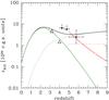 |
Fig. 1 Highest emissivity at the H I Lyman limit vs. redshift. The red solid curve at z ≥ 5 is our benchmark case, consistent with the XRB limit |
Figure 1 shows ϵ912 Å given by Eq. (3). The emissivity at the Lyman limit is a most interesting quantity because it can be compared to diverse observational estimates existing in literature. Our benchmark case is shown as the red solid line starting from z = 5. Our limit is compared to the recent values of Giallongo et al. (2015) and to the values reported by Masters et al. (2012; shown as black data points and open triangles, respectively). An assessment of the reasons behind the discrepancy between these different results is beyond the scope of this Letter. Still, taking the Giallongo et al. (2015) ionising emissivity at face value, we must conclude that the associated AGNs basically saturate the observed XRB, as apparent from Fig. 1.
We also compared our estimate of ϵ912 Å with the “minimum reionisation model” of Haardt & Madau (2012). In Fig. 1 the overall Lyman limit emissivity of Haardt & Madau (2012) is shown, along with the separate contributions of AGNs and star forming galaxies. The AGN emissivity closely fits the results by Hopkins et al. (2007), while for galaxies Haardt & Madau (2012) assumed that the fraction of Lyman continuum photons leaking into the IGM is a strong increasing function of redshift. This model reionises H I by z ≃ 6.7 and He II by z ≃ 2.8. Although our estimate benchmark emissivity at z ≃ 5–6 is similar to that of the model of Haardt & Madau (2012), the approximately constant comoving behaviour of the latter compared to the steep decline we adopted here leads to the different outcome in terms of reionisation (see below). For this reason we tested the somewhat extreme case of a constant comoving emissivity. The resulting highest emissivity is lower than that of the reionisation model of Haardt & Madau (2012) by a factor of ≃4 at high-z.
In Fig. 2 we show the resulting volume fraction occupied by H II regions (Eq. (4)). Our benchmark case allows for a fraction ≲13% of the IGM to be ionised by AGNs by z ≳ 6, showing that AGNs alone cannot reionise the Universe. We checked that this conclusion holds in spite of the uncertainties of the parameters. QHII = 1 at z = 6 can be reached only for αox ≳ 1.7, or αox ≳ 1.5 assuming RII ≃ 1 (i.e., no obscured sources). These figures seem to be unlikely when compared to available data. Finally, the constant comoving case produces a more extended reionisation history, but it still can only account for ≲27% of the ionised volume at z ≳ 6. In this case, reionisation by z ≳ 6 requires a mean escape fraction from star-forming galaxies ≳10%.
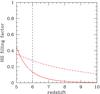 |
Fig. 2 Highest volume filling factor of H II vs. redshift. Curves as in Fig. 1. The dashed vertical line marks a fiducial reionisation redshift, z = 6. In our benchmark case the contribution to H II reionisation from AGNs is lower than 13%. |
It is interesting to note that the benchmark case (as well as the AGNs observed by Giallongo et al. 2015) would produce a H I ionisation rate consistent with z ≃ 5–6 data (e.g., Wyithe & Bolton 2011; Calverley et al. 2011), but it still falls short of reionsing the IGM at z ≳ 6 (Fig. 2). In other words, matching the observed level of the ionising background just below the ionisation redshift does not guarantee that a particular model is consistent with the entire reionisation history of the IGM.
A final comment concerns He II reionisation. Although a detailed assessment of this process is beyond the scope of this Letter, an AGN-dominated background would certainly lead to an extended reionisation epoch. This may agree with the recent claim of Worseck et al. (2014), but it may be in conflict with the sharp increase of the IGM temperature at mean cosmic density observed in the range 2 ≲ z ≲ 4 (Schaye et al. 2000; Becker et al. 2011; Bolton et al. 2012, 2014; Boera et al. 2014).
5. Conclusions
Under reasonable assumptions, we have shown that a population of unobscured, UV-emitting AGNs at z ≳ 5, if leading H I reionisation, would exceed observational constraints derived from the unresolved fraction of the X-ray background. Even a constant comoving emissivity at high-z would not be enough to produce an AGN-dominated ionising background. AGNs can account for a fraction of the ionising photon budget ≲13%, calling for a dominant contribution from star-forming galaxies. Given the observational constraints (e.g., Bouwens et al. 2011) on the galaxy population at high-z, this in turns requires a large mean escape fraction (≳10%).
Acknowledgments
We thank A. Comastri, P. Madau, A. Moretti for many fruitful discussions, and E. Giallongo for allowing us to use their results before publication.
References
- Becker, G. D., Rauch, M., & Sargent, W. L. W. 2007, ApJ, 662, 72 [NASA ADS] [CrossRef] [Google Scholar]
- Becker, G. D., Bolton, J. S., Haehnelt, M. G., & Sargent, W. L. W. 2011, MNRAS, 410, 1096 [NASA ADS] [CrossRef] [Google Scholar]
- Boera, E., Murphy, M. T., Becker, G. D., & Bolton, J. S. 2014, MNRAS, 441, 1916 [NASA ADS] [CrossRef] [Google Scholar]
- Bolton, J. S., Becker, G. D., Raskutti, S., et al. 2012, MNRAS, 419, 2880 [NASA ADS] [CrossRef] [Google Scholar]
- Bolton, J. S., Becker, G. D., Haehnelt, M. G., & Viel, M. 2014, MNRAS, 438, 2499 [NASA ADS] [CrossRef] [Google Scholar]
- Bouwens, R. J., Illingworth, G. D., Oesch, P. A., et al. 2011, ApJ, 737, 90 [NASA ADS] [CrossRef] [Google Scholar]
- Calverley, A. P., Becker, G. D., Haehnelt, M. G., & Bolton, J. S. 2011, MNRAS, 412, 2543 [NASA ADS] [CrossRef] [Google Scholar]
- Civano, F., Brusa, M., Comastri, A., et al. 2011, ApJ, 741, 91 [NASA ADS] [CrossRef] [Google Scholar]
- Dijkstra, M., Haiman, Z., & Loeb, A. 2004, ApJ, 613, 646 [NASA ADS] [CrossRef] [Google Scholar]
- Fan, X., Carilli, C. L., & Keating, B. 2006, ARA&A, 44, 415 [NASA ADS] [CrossRef] [Google Scholar]
- Faucher-Giguère, C.-A., Lidz, A., Hernquist, L., & Zaldarriaga, M. 2008, ApJ, 682, L9 [NASA ADS] [CrossRef] [Google Scholar]
- Fiore, F., Puccetti, S., Grazian, A., et al. 2012, A&A, 537, A16 [NASA ADS] [CrossRef] [EDP Sciences] [Google Scholar]
- Giallongo, E., Grazian, A., Fiore, F., et al. 2015, A&A, in press 10.1051/0004-6361/201425334 [Google Scholar]
- Gilli, R., Comastri, A., & Hasinger, G. 2007, A&A, 463, 79 [NASA ADS] [CrossRef] [EDP Sciences] [Google Scholar]
- Gilmore, R. C., Madau, P., Primack, J. R., Somerville, R. S., & Haardt, F. 2009, MNRAS, 399, 1694 [Google Scholar]
- Glikman, E., Djorgovski, S. G., Stern, D., et al. 2011, ApJ, 728, L26 [NASA ADS] [CrossRef] [Google Scholar]
- Gnedin, N. Y. 2000, ApJ, 535, 530 [NASA ADS] [CrossRef] [Google Scholar]
- Haardt, F., & Madau, P. 1996, ApJ, 461, 20 [NASA ADS] [CrossRef] [Google Scholar]
- Haardt, F., & Madau, P. 2012, ApJ, 746, 125 [NASA ADS] [CrossRef] [Google Scholar]
- Hinshaw, G., Larson, D., Komatsu, E., et al. 2013, ApJS, 208, 19 [NASA ADS] [CrossRef] [Google Scholar]
- Hiroi, K., Ueda, Y., Akiyama, M., & Watson, M. G. 2012, ApJ, 758, 49 [NASA ADS] [CrossRef] [Google Scholar]
- Hopkins, P. F., Richards, G. T., & Hernquist, L. 2007, ApJ, 654, 731 [NASA ADS] [CrossRef] [Google Scholar]
- Ikeda, H., Nagao, T., Matsuoka, K., et al. 2011, ApJ, 728, L25 [NASA ADS] [CrossRef] [Google Scholar]
- Jarosik, N., Bennett, C. L., Dunkley, J., et al. 2011, ApJS, 192, 14 [NASA ADS] [CrossRef] [Google Scholar]
- Lusso, E., Comastri, A., Vignali, C., et al. 2010, A&A, 512, A34 [NASA ADS] [CrossRef] [EDP Sciences] [Google Scholar]
- Madau, P., Haardt, F., & Rees, M. J. 1999, ApJ, 514, 648 [NASA ADS] [CrossRef] [Google Scholar]
- Marchese, E., Della Ceca, R., Caccianiga, A., et al. 2012, A&A, 539, A48 [NASA ADS] [CrossRef] [EDP Sciences] [Google Scholar]
- Masters, D., Capak, P., Salvato, M., et al. 2012, ApJ, 755, 169 [NASA ADS] [CrossRef] [Google Scholar]
- McQuinn, M. 2012, MNRAS, 426, 1349 [NASA ADS] [CrossRef] [Google Scholar]
- Meiksin, A. 2005, MNRAS, 356, 596 [NASA ADS] [CrossRef] [Google Scholar]
- Merloni, A., Bongiorno, A., Brusa, M., et al. 2014, MNRAS, 437, 3550 [NASA ADS] [CrossRef] [Google Scholar]
- Miralda-Escude, J., & Ostriker, J. P. 1990, ApJ, 350, 1 [NASA ADS] [CrossRef] [Google Scholar]
- Moretti, A., Vattakunnel, S., Tozzi, P., et al. 2012, A&A, 548, A87 [NASA ADS] [CrossRef] [EDP Sciences] [Google Scholar]
- Robertson, B. E., & Ellis, R. S. 2012, ApJ, 744, 95 [NASA ADS] [CrossRef] [Google Scholar]
- Robertson, B. E., Ellis, R. S., Dunlop, J. S., McLure, R. J., & Stark, D. P. 2010, Nature, 468, 49 [NASA ADS] [CrossRef] [PubMed] [Google Scholar]
- Salvaterra, R., Haardt, F., & Ferrara, A. 2005, MNRAS, 362, L50 [NASA ADS] [CrossRef] [Google Scholar]
- Salvaterra, R., Haardt, F., & Volonteri, M. 2007, MNRAS, 374, 761 [NASA ADS] [CrossRef] [Google Scholar]
- Salvaterra, R., Haardt, F., Volonteri, M., & Moretti, A. 2012, A&A, 545, L6 [NASA ADS] [CrossRef] [EDP Sciences] [Google Scholar]
- Schaye, J., Theuns, T., Rauch, M., Efstathiou, G., & Sargent, W. L. W. 2000, MNRAS, 318, 817 [NASA ADS] [CrossRef] [Google Scholar]
- Silverman, J. D., Green, P. J., Barkhouse, W. A., et al. 2008, ApJ, 679, 118 [NASA ADS] [CrossRef] [Google Scholar]
- Songaila, A. 2004, AJ, 127, 2598 [NASA ADS] [CrossRef] [Google Scholar]
- Steffen, A. T., Strateva, I., Brandt, W. N., et al. 2006, AJ, 131, 2826 [NASA ADS] [CrossRef] [Google Scholar]
- Telfer, R. C., Zheng, W., Kriss, G. A., & Davidsen, A. F. 2002, ApJ, 565, 773 [NASA ADS] [CrossRef] [Google Scholar]
- Trac, H., & Cen, R. 2007, ApJ, 671, 1 [NASA ADS] [CrossRef] [Google Scholar]
- Ueda, Y., Akiyama, M., Ohta, K., & Miyaji, T. 2003, ApJ, 598, 886 [NASA ADS] [CrossRef] [Google Scholar]
- Ueda, Y., Akiyama, M., Hasinger, G., Miyaji, T., & Watson, M. G. 2014, ApJ, 786, 104 [NASA ADS] [CrossRef] [Google Scholar]
- Van den Berk, D. E., Richards, G. T., Bauer, A., et al. 2001, AJ, 122, 549 [NASA ADS] [CrossRef] [Google Scholar]
- Vanzella, E., Siana, B., Cristiani, S., & Nonino, M. 2010, MNRAS, 404, 1672 [NASA ADS] [Google Scholar]
- Worseck, G., Prochaska, J. X., Hennawi, J. F., & McQuinn, M. 2014 [arXiv:1405.7405] [Google Scholar]
- Wyithe, J. S. B., & Bolton, J. S. 2011, MNRAS, 412, 1926 [NASA ADS] [CrossRef] [Google Scholar]
- Wyithe, J. S. B., & Loeb, A. 2003, ApJ, 586, 693 [NASA ADS] [CrossRef] [Google Scholar]
- Xue, Y. Q., Luo, B., Brandt, W. N., et al. 2011, ApJS, 195, 10 [NASA ADS] [CrossRef] [Google Scholar]
All Figures
|
Fig. 1 Highest emissivity at the H I Lyman limit vs. redshift. The red solid curve at z ≥ 5 is our benchmark case, consistent with the XRB limit |
| In the text | |
|
Fig. 2 Highest volume filling factor of H II vs. redshift. Curves as in Fig. 1. The dashed vertical line marks a fiducial reionisation redshift, z = 6. In our benchmark case the contribution to H II reionisation from AGNs is lower than 13%. |
| In the text | |
Current usage metrics show cumulative count of Article Views (full-text article views including HTML views, PDF and ePub downloads, according to the available data) and Abstracts Views on Vision4Press platform.
Data correspond to usage on the plateform after 2015. The current usage metrics is available 48-96 hours after online publication and is updated daily on week days.
Initial download of the metrics may take a while.