| Issue |
A&A
Volume 575, March 2015
|
|
|---|---|---|
| Article Number | A115 | |
| Number of page(s) | 12 | |
| Section | Stellar atmospheres | |
| DOI | https://doi.org/10.1051/0004-6361/201425316 | |
| Published online | 06 March 2015 | |
A comprehensive analysis of the magnetic standard star HD 94660: Host of a massive compact companion?⋆
1 Max-Planck Insitut für Extraterrestrische Physik, Giessenbachstrasse 1, 85748 Garching, Germany
e-mail: This email address is being protected from spambots. You need JavaScript enabled to view it.
2 ESO, Karl-Schwarzschild-Strasse 2, 85748 Garching, Germany
3 Armagh Observatory, College Hill, Armagh, BT61 9DG, Northern Ireland, UK
4 Department of Physics and Astronomy, The University of Western Ontario, London, Ontario, N6A 3K7, Canada
Received: 11 November 2014
Accepted: 24 January 2015
Abstract
Aims. Detailed information about the magnetic geometry, atmospheric abundances and radial velocity variations has been obtained for the magnetic standard star HD 94660 based on high-dispersion spectroscopic and spectropolarimetric observations from the UVES, HARPSpol and ESPaDOnS instruments.
Methods. We perform a detailed chemical abundance analysis using the spectrum synthesis code ZEEMAN for a total of 17 elements. Using both line-of-sight and surface magnetic field measurements, we derive a simple magnetic field model that consists of dipole, quadrupole and octupole components.
Results. The observed magnetic field variations of HD 94660 are complex and suggest an inhomogeneous distribution of chemical elements over the stellar surface. This inhomogeneity is not reflected in the abundance analysis, from which all available spectra are modelled, but only a mean abundance is reported for each element. The derived abundances are mostly non-solar, with striking overabundances of Fe-peak and rare-earth elements. Of note are the clear signatures of vertical chemical stratification throughout the stellar atmosphere, most notably for the Fe-peak elements. We also report on the detection of radial velocity variations with a total range of 35 km s-1 in the spectra of HD 94660. A preliminary analysis shows the most likely period of these variations to be of order 840 d and, based on the derived orbital parameters of this star, suggests the first detection of a massive compact companion for a main sequence magnetic star.
Conclusions. HD 94660 exhibits interestingly complex magnetic field variations and remarkable radial velocity variations. Long term monitoring is necessary to provide further constraints on the nature of these radial velocity variations. Detection of a companion will help establish the role of binarity in the origin of magnetism in stars with radiative envelopes.
Key words: stars: abundances / stars: magnetic field / stars: chemically peculiar / binaries: spectroscopic
Based in part on our own observations made with the European Southern Observatory (ESO) telescopes under the ESO programme 093.D-0367(A) and programmes 076.D-0169(A), 088.D-0066(A), 087.D-0771(A), 084.D-0338(A), 083.D-1000(A) and 60.A-9036(A), obtained from the ESO/ST-ECF Science Archive Facility. It is also based in part on observations carried out at the Canada-France-Hawaii Telescope (CFHT) which is operated by the National Research Council of Canada, the Institut National des Science de l’Univers of the Centre National de la Recherche Scientifique of France and the University of Hawaii.
© ESO, 2015
1. Introduction
Of order 10% of main sequence A and B stars are magnetic. For the majority of these stars, their magnetic properties are studied using circular polarisation spectra, which provide a measure of the mean magnetic field projected along the line-of-sight (⟨ Bz ⟩). A fraction of these stars rotate slowly and/or have strong enough magnetic fields that Zeeman splitting is observed in individual lines of the intensity (Stokes I) spectra (see Bailey, 2014, and references therein). The magnitude of this splitting provides a measure of the mean magnetic field modulus at the stellar surface (⟨ B ⟩). These magnetic A and B stars exhibit anomalous atmospheric abundances and are referred to as the chemically peculiar A– type (Ap) stars. These stars often have ⟨ Bz ⟩ in excess of about 1 kG and ⟨ B ⟩ of order several thousands to tens of thousands of gauss (e.g. Donati & Landstreet, 2009).
The chemical peculiarities of Ap stars can be quite striking. For example, the Fe-peak element Cr may be as much as 102 times overabundant compared to the Sun. Still more impressive are the abundances of rare-earth elements, which are commonly in excess of solar values by as much as 104 times.
Ap stars may be highly variable, with their magnetic field strengths and spectral line strengths and shapes varying with the rotation period of the star. This variability is best explained via the rigid rotator model (see Stibbs, 1950). In this model, the line-of-sight and magnetic axes are at angles i and β to the rotation axis, respectively. Therefore, different magnetic field measurements throughout the rotation cycle of the star are the result of observing the field at different orientations and since chemical elements are distributed non-uniformly and non-axisymmetrically over the stellar surface, spectrum variability is also observed (Ryabchikova, 1991).
HD 94660 (=HR 4263) is a bright (V = 6.11) chemically peculiar magnetic Ap star that is commonly used as a magnetic standard to test polarimetric systems in the southern hemisphere. The field was first discovered by Borra & Landstreet (1975) using an Hα magnetograph; they reported a value for the line-of-sight magnetic field of ⟨ Bz ⟩ = −3300 ± 510 G. HD 94660 is a sharp-lined star with clearly resolved Zeeman splitting in several spectra lines (Mathys, 1990). Bohlender et al. (1993) report a projected rotational velocity of vsini< 6 km s-1 and a roughly constant line-of-sight magnetic field strength of ⟨ Bz ⟩ = −2520 G, based on measurements using Hβ. A period of rotation of order 2700 d was first proposed by Hensberge (1993) and later discussed by Mathys et al. (1997) with respect to ⟨ B ⟩ data. More recently, Landstreet et al. (2014) studied the field variations of HD 94660 from 17 FORS1 observations taken over a 6 yr period from 2002 to 2008. They find a peak-to-peak variation in ⟨ Bz ⟩ of about 800 G, ranging from about −2700 and −1900 G. From these variations, a rotation period of 2800 ± 250 d is deduced, which agrees with previous determinations.
Landstreet & Mathys (2000) were the first to report clear ⟨ Bz ⟩ variations (between about −1800 and −2100 G) which, together with ⟨ B ⟩ data from Mathys & Hubrig (1997), enabled them to model the magnetic field of this star using a colinear multipole expansion. They adopted a model that consists of dipole, quadrupole and octupole components with surface polar field strengths of −8400, 2700 and 6900 G, respectively. As seen above, the value of ⟨ Bz ⟩ is always negative, indicating that i + β ≲ 90° i.e. only the negative magnetic pole is observed. This is confirmed by this model where the determined values for i and β are 5° and 47°. We point out that, in general, this model does provide a rough first approximation to the field variations.
In this paper, we discuss efforts to model the magnetic field and chemical abundances of many elements based on high-dispersion, polarimetric spectra. The following section discusses the observations. Section 3 outlines the derived physical parameters; Sect. 4 discusses the magnetic field measurements and model; Sects. 5 and 6 describe the modelling technique and abundance analysis, respectively; Sect. 7 reports detected radial velocity variations; and Sect. 8 summarises the results of the paper.
Summary of the stellar and magnetic properties of HD 94660.
2. Observations
We have acquired one spectropolarimetric observation of HD 94660 and have retrieved an additional seven archival spectra that were utilised in this study, all of which were taken with HARPSpol. This is a high-resolution (R ≃ 115 000), cross-dispersed echelle spectropolarimeter that covers a spectral range between 3780–6910 Å and is mounted on the European Southern Observatory (ESO) 3.6-m telescope located at La Silla. The high signal-to-noise ratio (S/N) observations consist of 6 circularly polarised Stokes V spectra (with the 01-04-2012 observation also including linear polarisation in both Stokes Q and U), and two unpolarised Stokes I spectra, all acquired between May 2009 and April 2014. Each polarimetric observation (except for the observation taken on 31-05-2009) was obtained by acquiring four successive individual spectra with the quarter-wave plate rotated in such a way to acquire the desired Stokes spectrum (see e.g. Rusomarov et al., 2013,for further details).
The HARPSpol spectra were reduced using a modified version of the REDUCE package (Piskunov & Valenti, 2002; Makaganiuk et al., 2011). Wavelength calibration was performed using the spectrum of a ThAr calibration lamp and then corrected to the heliocentric rest frame. Normalisation of the spectra was achieved by first dividing the spectra by the optimally-extracted spectrum of the flat-field to correct for the blaze shape and fringing. The resulting spectra were then corrected by the response function derived from observations of the Sun. The last step involved fitting a smooth, slowly-varying function to the envelope of the entire spectrum. The final output is a set of continuum-normalised Stokes I spectra, the Stokes parameter of interest (V,Q,U) and a diagnostic null spectrum that is calculated in such a way that the polarisation cancels out, which often allows us to identify spurious signals that are present in the processed data. The spectrum that was acquired on 31-05-2009 only completed half of the full polarimetric sequence, which enables the cancellation of first order (linear) wavelength drift, but does not correct for second order (quadratic) drift and does not allow the computation of a diagnostic null spectrum. We also note that the retarder angles listed in the observations obtained on 05-01-2010 were inconsistent with the usually adopted values for obtaining Stokes V measurements and are likely erroneous. We therefore proceeded to reduce the data assuming the usual retarder angles for the sequence of observations, and then verified that the resulting polarised and unpolarised spectra were in good agreement with the other observations.
In addition to the HARPSpol observations, we identified another archival, circularly polarised, high-resolution (R ≃ 65 000) spectropolarimetric observation acquired with ESPaDOnS on January 9, 2006. ESPaDOnS, which is mounted at the 3.6 m Canada-France-Hawaii Telescope (CFHT), is also a bench-mounted, cross-dispersed echelle spectropolarimeter, which covers a broader spectral range compared to HARPSpol of 3690–10 481 Å. The polarimetric observation was obtained by taking a sequence of four sub-exposures with different positions of the Fresnel Rhomb to acquire a single Stokes V spectrum, according to the procedure described by Donati et al. (1997). The ESPaDOnS spectra were processed using the automated reduction package LIBRE-ESPRIT, following the double-ratio procedure (Donati et al., 1997).
Lastly, we also found three nights of archival UVES data consisting of a total of 11 spectra. UVES is a cross-dispersed spectrograph mounted on the ESO 8.2-m Very Large Telescope (VLT) located at Paranal. It has both a blue and red arm offering different spectral resolutions and wavelength coverages. The blue arm offers R up to about 80 000 and a spectral range of 3100–4900 Å, whereas the red arm covers 4800–10 200 Å with R up to about 110 000. Table 2 summarises our entire collection of spectra for HD 94660.
Log of available spectra for HD 94660.
3. Physical parameters
3.1. Effective temperature and gravity
Geneva and Strömgren uvbyβ photometry are available for HD 94660 and both were utilised to determine the effective temperature Teff and gravity log g for the star. For the Geneva photometry, we used the FORTRAN code developed by Kunzli et al. (1997). A modified version of the Napiwotzki et al. (1993) code, that corrects the effective temperature to the Ap temperature scale (see Landstreet et al., 2007, for a complete discussion), was used for the Strömgren photometry.
From the Geneva and Strömgren photometric systems, we found Teff = 11 500 K, log g = 4.10 and Teff = 11 100 K, log g = 4.26, respectively. We adopt the mean of these two sets of values for our analysis with Teff = 11 300±400 K and log g = 4.18±0.2, with the uncertainties estimated from the scatter between the measurements, and by taking into account the intrinsic uncertainties in computing these parameters for Ap stars. These parameters are used for our abundance analysis (see Sect. 6).
3.2. Luminosity, stellar radius and mass
van Leeuwen (2007) reports a Hipparcos parallax of 6.67 ± 0.80 milliarcseconds. From this value, a distance to HD 94660 of about 150 pc is deduced. With a well determined distance, an appropriate bolometric correction for Ap stars can be used to determine the stellar luminosity (see Landstreet et al., 2007), which is found to be log L/L⊙ = 1.97 ± 0.25 with uncertainties propagated in the usual way.
Based on the Teff and luminosity determinations, it is straightforward to compute a stellar radius of R = 2.53 ± 0.37 R⊙. By further comparing the position of HD 94660 to theoretical evolutionary tracks (Girardi et al., 2000) in an HR diagram, we are able to estimate the star’s evolutionary mass. Using the adopted uncertainties in Teff and L, we proceed by comparing the star’s position to multiple evolutionary tracks of varying masses. In this manner, we estimate that HD 94660 has a mass of about 3.0 ± 0.20 M⊙. This is in agreement to the mass of 3.51 ± 0.64 M⊙ that we can estimate from the stellar radius and photometrically determined log g. Further, the position in the HR diagram suggests that HD 94660 has completed less than half of its main sequence lifetime. This is consistent with Landstreet et al. (2008), who find strong magnetic fields only in young Ap stars.
4. Magnetic field
Log of the line-of-sight surface field, ⟨ Bz ⟩, measurements of HD 94660.
4.1. Longitudinal magnetic field measurements
For each of the Stokes V spectra we measured the mean, surface-averaged longitudinal magnetic field (⟨ Bz ⟩) from line-averaged least-squares deconvolved (LSD; Donati et al., 1997) line profiles. The technique involves obtaining mean line profiles by combining all spectral lines in a given line list (normally metallic and He lines). The result is a much higher S/N with the ability to detect weaker Zeeman signatures due to magnetic fields. ⟨ Bz ⟩ was measured using the first-order moment method discussed by Rees & Semel (1979), and as implemented by Donati et al. (1997) and Wade et al. (2000) according to the equation: ![Mathematical equation: \begin{equation} \langle \mathit{B}_z \rangle = \frac{-2.14 \times 10^{11}}{\lambda z c }\frac{\int{(v - v_0)V(v){\rm d}v}}{\int{[1-I(v)]{\rm d}v}}\cdot \label{b_eq} \end{equation}](/articles/aa/full_html/2015/03/aa25316-14/aa25316-14-eq104.png) (1)In this equation, v is the velocity within the LSD profile, V(v) is the continuum-normalised Stokes I profile and I(v) is the continuum-normalised intensity profile. The wavelength λ (in nm) and Landé factor z correspond to the weighting factors used in the calculation of the LSD profiles (500-nm and 1.2, respectively).
(1)In this equation, v is the velocity within the LSD profile, V(v) is the continuum-normalised Stokes I profile and I(v) is the continuum-normalised intensity profile. The wavelength λ (in nm) and Landé factor z correspond to the weighting factors used in the calculation of the LSD profiles (500-nm and 1.2, respectively).
The LSD profiles were extracted using the iLSD code of Kochukhov et al. (2010). As input the code requires a line mask that was extracted from the Vienna Atomic Line Database (VALD; Kupka et al., 1999, 2000; Ryabchikova et al., 1997; Piskunov et al., 1995) for the spectral range covered by HARPS, using the mean abundances determined in this work and discussed in Sect. 6. This linelist was used for both the HARPS and ESPaDOnS spectra to provide a consistent ⟨ Bz ⟩ measurement between the two datasets. We then proceeded to remove all lines that were blended with lines not used in this analysis, such as broad hydrogen lines or lines blended with strong telluric absorption bands. As a final step we then automatically adjust the line depths from their theoretical predictions to provide a best fit to the observed Stokes I spectrum, while also removing lines that are poorly fit (such as those lines that show very strong Zeeman splitting). This final mask was then used to extract mean line profiles for all spectra that we label as “full mask”. We also extracted mean line profiles of individual elements for Si, Ti, Cr, Fe and Nd, using the multi-profile capabilities of iLSD. In each case we provided two input masks based on our final full mask, one made entirely of the element of interest and the other containing all other lines. Both masks are used simultaneously as input and allow us to extract a representative mean, unblended profile of the element of interest. All LSD profiles were extracted onto a 1.8 km s-1 velocity grid and uncertainties were computed by propagating the uncertainties in the final LSD profiles.
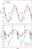 |
Fig. 1 ⟨ Bz ⟩ and ⟨ B ⟩ variations of HD 94660. The solid black lines are the adopted magnetic field model variations from Sect. 4.3. Top: ⟨ Bz ⟩ LSD measurements using the full mask (black circles) and Nd mask (green triangles). Note that the open and filled symbols denote measurements from the ESPaDOnS spectrum and HARPSpol spectra, respectively. Balmer line measurements from Landstreet et al. (2014) are the filled red squares. Bottom: phased ⟨ B ⟩ measurements from Fe ii 6149 (blue squares), Cr ii 6833 (red triangles) and Nd iii 6145 (green circles). The dotted green line is the best-fit sinusoidal variations to the Nd measurements. |
Our final measurements are listed in Table 3. The top panel of Fig. 1 plots the ⟨ Bz ⟩ measurements against rotational phase for the full metallic and Nd masks as well as the magnetic field model derived in Sect. 4.3. Also shown are the Balmer line measurements of Landstreet et al. (2014). Although the HARPSpol and ESPaDOnS magnetic data have not been intercalibrated for this star, we note that the consistency between the ESPaDOnS and HARPSpol measurements is satisfactory. Furthermore, previous studies have shown a good agreement between the polarimetric spectra acquired with ESPaDOnS and HARPSpol (Piskunov et al., 2011).
4.1.1. Measurements from individual spectral lines
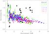 |
Fig. 2 Variations in magnetic field strength ⟨ Bz ⟩ versus EQW for individual spectral lines. Different symbols denote different elements, while different colours are used to represent different Landé factor ranges. Note that the absolute value of the field strength is shown and each measurement has been normalised as discussed in the text. The dashed line is a linear fit to the data. |
The extremely sharp lines and strong magnetic field result in clean, strong Stokes V signatures for individual spectral lines. This allows us to test the multi-line technique of LSD (see Sect. 4.1) by measuring ⟨ Bz ⟩ from individual lines of elements. We performed these measurements for a total of about 80 unblended lines which included the elements Si, Ti, Cr, Fe and Nd (the same elements for which we performed LSD to compute the field from individual elements). In general, the measurements agree with the values we derive and present in Table 3, but with large scatter between different lines of an individual element. In an attempt to understand this scatter, we plot the measured ⟨ Bz ⟩ value against the equivalent width (EQW) for all the spectral lines (see Fig. 2). To account for any variation in the field measurements due to the different phases, all values have been normalised by the ⟨ Bz ⟩ and EQW value for the Fe i 4982 line obtained for a given night. Note that the absolute value of the field strength is shown for clarity.
The results show a clear trend, namely a stronger field strength for lines with smaller EQW and a weaker field strength for lines with larger EQW. We note that almost all of the outliers from this trend were lines with very small Landé factors. These results are difficult to interpret. On one hand, this result could reflect differential desaturation i.e. that strong lines should be more sensitive to the desaturation of the line due to magnetic splitting and so the relative change in the EQW of that line should be greater than for a weak line in the presence of a strong magnetic field. We attempted to test this hypothesis by producing a synthetic spectrum using ZEEMAN.F (see Sect. 5), which includes all of the measured spectral lines. Because the field strength is kept constant for a given phase in ZEEMAN.F for all lines, any systematic change in the measured ⟨ Bz ⟩ value as a function of the EQW can be attributed to differential saturation. Unfortunately, the results we derived from this test are also difficult to interpret, but it appears that the general trend of the synthetic tests do not agree with the results from the observations. Another possible explanation caused by differential saturation is that this result could simply reflect small systematic changes in the measured centre-of-gravity of Stokes V (the numerator in Eq. (1)). This would predominantly affect strong lines with complex splitting patterns, resulting in a blended profile that does not have the same centre-of-gravity as the unsaturated line with the same splitting pattern.
On the other hand, this result could be unrelated to saturation effects and could be a measure of the change of the decreasing field strength with increasing vertical height in the atmosphere: the cores of weak lines are formed deeper in the atmosphere and should have intrinsically stronger fields relative to strong lines with cores formed higher. Using our ZEEMAN.F model to estimate the depth of the atmosphere (~0.6% of the stellar radius), we compute an expected change of the order of ~4% between the measured field strength of lines formed at the top and bottom of the atmosphere. Figure 2 shows a typical variation in the strength of the magnetic field of order 30% from weak to strong lines (closer to 50% if you consider the extreme values). Therefore, it seems unlikely that this effect is important and the nature of this trend is still unclear.
Log of surface field, ⟨ B ⟩, measurements of HD 94660.
4.2. Surface magnetic field measurements
The sharp-lined features and high resolving powers of the HARPSpol, UVES and ESPaDOnS instruments allowed us to make measurements of the mean field moduli (⟨ B ⟩) from observed Zeeman splitting in the lines of Nd iiiλ6145, Fe iiλ6149 and Cr iiλ6833. Notable exceptions are for the one ESPaDOnS spectrum and two nights of UVES spectra. The lower resolving power of ESPaDOnS compared to HARPSpol did not allow us to see sufficient splitting in Nd iii, whereas insufficient wavelength coverage for the UVES spectra did not allow for measurements of splitting in Cr ii (on 01-05-2011) or Nd iii and Fe ii (on 01-08-2011).
To obtain values of ⟨ B ⟩, the atomic data from the VALD database was used and the field strength calculated from the equation 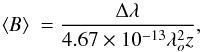 (2)where Δλ denotes the shift of the σ components from the zero field wavelength, λo is the rest wavelength in Å and z is the effective Landé factor of the line (1.00, 1.34 and 1.33 for λ6145, 6149 and 6833, respectively). The separation of the elements of the Zeeman split lines that determine Δλ was measured by fitting Gaussians to each component using the splot function in IRAF. The uncertainties were estimated by considering the dispersion between a series of measurements of ⟨ B ⟩ from multiple Gaussian fits to each component. Bailey et al. (2011) note that measurements of ⟨ B ⟩ from Eq. (2) are very sensitive to small changes in Δλ. Because of the high resolution and essentially zero rotation rate of HD 94660, the dispersion in our measurements of Δλ is less than about 0.005 Å in most cases. Table 4 summarises these ⟨ B ⟩ measurements and the bottom panel of Fig. 1 show the phased rotational variations of the surface fields from the three elements.
The scatter of ⟨ B ⟩ values around the mean curve confirms that our uncertainty estimates are reasonable. The consistency of measurements from each individual element taken on successive nights (24-05-2009 and 25-05-2009) and the agreement, within estimated uncertainties, between ⟨ B ⟩ measurements of the Fe-peak elements Cr ii and Fe ii (except for a single measurement) further suggests that the quoted uncertainties are realistic. The surface field appears to vary sinusoidally; however, the average surface field from the Fe-peak elements is of order 400 G larger than that of Nd iii. Further, the peak-to-peak amplitude of the variations is twice as large for Nd iii (of order 800 G) compared to the Fe-peak elements (of order 400 G). The fact that different elements sample the field in significantly different ways suggest that the abundance distributions of different elements, in addition to the field structure, are inhomogeneous over the stellar surface. This is further supported by the discrepant ⟨ Bz ⟩ measurements of different elements discussed above and listed in Table 3.
4.3. Magnetic field model
Given the long rotation period of HD 94660, we are fortunate to have sufficient phase coverage for both ⟨ Bz ⟩ and ⟨ B ⟩ in order to derive a simple magnetic field model. In general, the FORS1 data show that the Balmer line and metallic line ⟨ Bz ⟩ measurements agree closely, except for one discrepant metal ⟨ Bz ⟩ value (Landstreet et al., 2014). However, a large discrepancy exists between all FORS1 measurements and those from high-resolution spectra. In particular, the FORS1 data show a much larger range in ⟨ Bz ⟩. This can be seen in the top panel of Fig. 1 where the FORS1 Balmer line measurements vary by order 800 G whereas the full LSD mask from the high resolution spectra vary by about 300 G. We opt for using the Balmer line ⟨ Bz ⟩ variations as discussed by Landstreet et al. (2014) to derive a field geometry. We point out that this is the main reason for the discrepancy between our field structure (see below) and the one derived by Landstreet & Mathys (2000).
The FORTRAN program FLDSRCH.F (Landstreet & Mathys, 2000) derives a magnetic field geometry based on the observed ⟨ Bz ⟩ and ⟨ B ⟩ variations. It produces a simple co-axial multipole expansion that consists of dipole (Bd), quadrupole (Bq) and octupole (Boct) components with the angles between the line-of-sight and rotation axis (i) and the magnetic field and rotation axes (β), specified. For HD 94660, a new field geometry with i = 16°, β = 30°, Bd = −7500 G, Bq = −2000 G, and Boct = 7500 G is found. The phased ⟨ Bz ⟩ and ⟨ B ⟩ variations using our adopted geometry are shown in Fig. 1 and are in good agreement with the longitudinal field variations measured by Landstreet et al. (2014) from FORS1, as well as the measured Fe-peak surface field variations.
Although our magnetic field model is based on the fit to the large amplitude ⟨ Bz ⟩ FORS1 data, it is nevertheless useful to compare our geometry to the one from Landstreet & Mathys (2000) because it is not entirely clear which, if either, is better to use. In general, our adopted field geometry is not drastically different than the one proposed by Landstreet & Mathys (2000; see Sect. 1). The angles i + β are roughly the same, although the individual values of these angles differ (recall that i and β can be interchanged). The values of Bd and Boct are similar; however, the relatively small Bq, although comparable in magnitude, is negative in our derived geometry and positive in the geometry of Landstreet & Mathys (2000). The circular polarisation signatures in Stokes V are also well produced with both geometries. Figure 3 compares the observed and synthetic Stokes I and V profiles, using both models, for Nd iii λ6145 (note that only one phase is shown but the splitting is equally well reproduced at all phases). It is obvious from this figure that both fields do an adequate job at reproducing the observed magnetic properties in the spectrum of HD 94660. Based on Fig. 3, it is unclear which model is best and both models are too coarse to describe the complex field variations over the visible stellar surface. Although our field model is preferred, we perform an abundance analysis using both geometries (see Sect. 5).
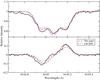 |
Fig. 3 A comparison of magnetic field models. In black are the observed Stokes I (top) and V (bottom) profiles for Nd iii λ6145 for the 28-08-2014 HARPSpol spectrum. We overplot the computed line profiles for our adopted magnetic field geometry (red dashed line) and the magnetic field geometry of Landstreet & Mathys (2000; blue dotted line). |
Landstreet & Mathys (2000) suggest that β is likely smaller than i for a very large fraction of slow rotators, arguing that for long period stars (P ≥ 25 d) it is equally likely for the rotation pole to be positioned anywhere on the visible hemisphere. For this reason, smaller values of i are statistically unlikely, since it would require i to be within a small region of the visible hemisphere. However, their geometries are based only on intensity and circular polarisation spectra which makes it difficult to distinguish i and β. Fortunately, we have available two observations of the linear polarisation (Stokes Q and U) spectra of HD 94660 taken with the HARPSpol instrument on 01-04-2012 (see Sect. 2). The linear polarisation data will allow us to distinguish which of the two angles is larger. Figure 4 compares the Stokes Q signature for our adopted magnetic field model, assuming that i>β (top panel) and i<β (bottom panel). For i>β, the model clearly predicts a Stokes Q signature that is too large compared to the observations. Alternatively, for i<β, the model predicts a much more modest signature, in relative agreement to what is observed, although we admit that the model does not accurately represent the true variations in linear polarisation for this star (we note that similar results are also seen with Stokes U and with the Landstreet & Mathys 2000 model). This figure strongly suggests that, contrary to the assumption of Landstreet & Mathys (2000), for HD 94660 β is the larger of these two angles for both models.
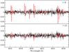 |
Fig. 4 A comparison of the Stokes Q signatures of synthetic models to the HARPSpol observation on 01-04-2012. In black is the observed Stokes Q spectrum. Overplotted is our adopted magnetic field model (red dashed line). The top panel assumes i>β, whereas the bottom assumes i<β. |
5. Spectrum synthesis program
5.1. ZEEMAN.F
The FORTRAN program ZEEMAN.F is a spectrum synthesis program developed by Landstreet (1988). ZEEMAN.F performs line formation and radiative transfer in a magnetic field. The input magnetic field geometry consists of the axisymmetric superposition of a dipole, quadrupole and octupole with specified values of the angles i and β. ZEEMAN.F interpolates an appropriate atmospheric model from a grid of solar abundance ATLAS9 models based upon the Teff and log g supplied. The atomic data needed for line synthesis are taken from the VALD database. ZEEMAN.F assumes a homogeneous abundance distribution vertically throughout the stellar atmosphere and computes all four Stokes parameters. ZEEMAN.F allows up to six abundance rings that are symmetric about the magnetic axis to be specified on the stellar surface, with each ring having equal extent in colatitude. Within each ring, a uniform abundance is assumed. For each modelled spectrum, a best-fit vsini and radial velocity vR are calculated.
5.2. Choice of magnetic field model
One of the major difficulties in performing the abundance analysis of a magnetic star is the inclusion of the effects of the magnetic field on spectral line formation. This is, in part, due to the limited number of tools that include this physics, but also because of the inherent ambiguity in selecting an appropriate magnetic field model. Section 4 highlighted this discrepancy with two apparently adequate field models to explain the observed Stokes I and V profiles of HD 94660. Therefore, we compared the abundances derived from these two magnetic field geometries. We also tested the abundances with a simple dipolar model in which the value of Bd was chosen to be approximately three times the largest observed ⟨ Bz ⟩ value (this leads to roughly the same extrema in the observed ⟨ Bz ⟩ and ⟨ B ⟩ values).
We note that the agreement between the different models is impressive. For any given set of fundamental parameters (i.e. Teff and log g), the difference in the derived abundances between the three models are generally less than about 0.1 dex and no worse than about 0.2 dex. It is encouraging that the choice of model does not drastically influence the final abundances. In fact, a very coarse model, consisting only of a dipole, can give accurate abundances, which suggests that the final abundances may not be very sensitive to the difference between these simple models and the real field distribution. Apparently, the inclusion a magnetic field model that roughly explains the ⟨ Bz ⟩ and ⟨ B ⟩ variations is sufficient to provide an accurate analysis. This lends support to studies such as the one by Bailey et al. (2014) for which simple dipolar models are used to quantify the evolution of atmospheric abundances in Ap stars. Since the abundances depend little on the magnetic field model, the following section reports only on abundances found using the field geometry we present in Sect. 4.3.
6. Elemental abundances
The abundances are measured with respect to H, and are tabulated with their associated uncertainties.
Insignificant variability in the strengths and shapes of most spectral lines is observed among the twelve spectra available to model for HD 94660. For lines that exhibit strong Zeeman signatures (for example Nd iii at 6145 Å) differences can be seen in the line structure (i.e. relative strengths of the σ and π components) and, in some cases, marginal changes in the line strength. However, line depth changes are limited to less than about 0.05 in intensity. Therefore, although all spectra are modelled, we report only a mean abundance for each element. Uncertainties are determined in two ways, depending upon the number of spectral lines available to model. For elements with multiple lines, the uncertainties are estimated from the observed scatter between the best-fit abundances. When only one (or few) lines are available to model, we estimate uncertainties by changing the best-fit abundance for each element until the reduced χ2 deviates from best-fit models by about 1 (i.e.  ). The uncertainty is then the difference between the two abundances and corresponds approximately to a 1σ uncertainty. Table 5 lists the abundances of each element, as well as the total number of lines modelled for each element. For reference, the solar abundance ratios are provided (Asplund et al., 2009). Figure 5 provides an example of the quality of fit for three spectral windows for the HARPSpol observation taken on April 28, 2014. Below, each element is discussed individually.
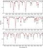 |
Fig. 5 Example of three synthesised spectral windows for the 28-04-2014 HARPSpol spectrum of HD 94660. The observed spectrum is in black (solid line) and the model is in red (dashed line). The bottom panel illustrates the vertical stratification of Fe in the atmosphere of HD 94660, where strong lines of Fe ii and weak lines of Fe i are fit well with the abundance of Table 5, but the weaker lines of Fe ii require an enhanced abundance to be well modelled. |
6.1. Helium
Many lines of helium exist to derive an abundance. He i λ4471 and λ5876 are predicted to be the strongest helium lines in the spectrum, but they are not detected in the available spectra. An upper limit for helium is derived from these regions that is at least a factor of 12 below the solar abundance. As expected of a magnetic Ap star, HD 94660 is He-weak.
6.2. Oxygen
The O i multiplet at 6155-56-58 Å is present in all spectra and is used to derive a mean abundance. The ESPaDOnS spectrum also includes the O i lines at 7771-74-75 Å, however, this triplet suffers from non-LTE effects and is therefore not considered. The adopted abundance is about 2.5 times less than in the Sun.
6.3. Magnesium
The only line suitable for modelling is Mg ii at 4481 Å. At all phases, this line is reasonably well fit with an abundance that is a factor of 4 below the solar ratio.
6.4. Silicon
Several clean lines of Si ii exist throughout the spectrum including strong lines at 5041 and 5055-56 Å, as well as the weaker line at 4621 Å. When fit simultaneously, λ5041, 5055-56 require an abundance that is about 0.5 dex less than that of λ4621. Table 5 reports the average of these abundances.
We also found a line of Si iii at 4552 Å. This line requires an abundance that is more than 10 times that of the mean abundance from the Si ii lines. This is exactly what was reported for a sample of mid to late B-type stars by Bailey & Landstreet (2013a), who argue that the discrepancy between the abundances derived from the first and second ionisation states of silicon is likely the result of strong vertical stratification in the stellar atmosphere. The different abundance values found using stronger and weaker lines of Si ii, and the line of Si iii, indicate that stratification is also likely in HD 94660.
6.5. Calcium
Possible useful lines of calcium at 8498, 8542 and 8662 Å are present in the ESPaDOnS spectrum, however, these are blended with the Paschen lines, which cannot be calculated correctly with Zeeman at present. Therefore, only Ca ii at 3933 Å was used to derive the final abundance of calcium. We note that distinctly different abundances are required to adequately fit the wings and core of this line (see Babel, 1992, where this effect is first explained for Ca). An abundance derived from the wings of this line, which are formed deeper in the atmosphere, suggest an abundance that is approximately solar. On the other hand, the core (formed higher up in the atmosphere) requires an abundance that is of order 0.8 dex below the solar abundance. This is a symptom of vertical stratification and it would appear calcium is strongly stratified throughout the atmosphere of HD 94660. The mean abundance of calcium is reported in Table 5.
6.6. Titanium
For deriving the mean abundance of titanium, there are several lines to choose throughout the blue spectrum. We have modelled the lines of Ti ii at 4533, 4549, 4563, 4568 and 4571 Å, and also at 4798 and 4805 Å. Each set of lines is synthesised separately and within each set the lines are modelled simultaneously. The final abundance is the mean of these two values (see Table 5).
The abundance that fits well the weaker lines of λ4568 and 4798, as well as the weak lines that are blended with other Fe-peak elements at λ4533 and 4549, is systematically too large for the stronger lines at λ4563, 4571 and 4805. This is a symptom of vertical stratification (Bagnulo et al., 2001). Nevertheless, Ti is clearly overabundant compared to the Sun by about a factor of 30.
6.7. Chromium
Unlike the other Fe-peak elements, the abundance derived for Cr is not as drastically dependent upon the lines modelled, which suggests that Cr may not be significantly stratified throughout the stellar atmosphere. This is illustrated in Fig. 5 where most lines of Cr ii (both strong and weak), as well as two lines of Cr i, are fit well with the same uniform abundance. Note that HD 94660 is relatively hot for the presence of neutral atoms, however, these lines are unambiguously detected in all modelled spectra and are predicted to be visible by ZEEMAN.F. Furthermore, tests of the depth of core formation for these lines indicate that they are formed in the upper part of the stellar atmosphere, where the temperature is necessarily cooler and consistent with the presence of neutral chromium. However, over 30 lines of Cr ii were tested throughout the spectrum with this uniform abundance, and a notable fraction of weaker lines require a larger abundance than is recorded in Table 5 to be adequately modelled. Although apparently not as significant as other elements, stratification may still be present for Cr. The final abundance of Cr was found by simultaneously fitting Cr ii lines at 4531, 4539, 4555, 4558, 4565, 4587, 4588, 4590 and 4592 Å. At all phases, Cr is modelled well with an abundance that is of order 300 times larger than the solar ratio.
6.8. Manganese
The abundance of Mn was derived from the pair of Mn ii lines at 6122 Å. The lines are well modelled at all phases with a uniform abundance that is of order 8 times larger than the solar abundance.
6.9. Iron
One mean abundance is not adequate to satisfactorily model all the spectral lines of Fe. It is clear from Fig. 5 that the adopted abundance fits the weaker lines well, but is systematically too large for the stronger Fe ii lines. This is evident throughout the spectrum, with well over 20 Fe lines modelled with the uniform abundance listed in Table 5. This is symptomatic of vertical stratification in the atmosphere. Multiple lines of Fe ii are used to compute the mean abundance of iron and the larger estimated uncertainty is indicative of the discrepancies found when modelling each line. The weaker Fe ii lines at 5029, 5031, 5032, 5034, 5035 and 5036 were fit simultaneously, and required an abundance larger by 0.6–0.7 dex than that deduced using strong lines such as 4583 and 5018 Å. Three lines of Fe i at 5014, 6136 and 6137 Å were also modelled and required a similar abundance to what is required to fit the stronger Fe ii lines. It is clear that Fe is at least of order 30 times more abundant than in the Sun.
6.10. Cobalt
The spectrum appears extraordinarily rich in Co ii. Several lines of Co ii are scattered throughout the spectrum. A total of eight lines were modelled: 5016, 5017, 5023, 5025, 5027, 5129, 5135, 5131 Å. All lines of Co ii are reasonably well modelled with a uniform abundance and suggest an abundance that is at least 300 times greater than that of the Sun.
The detection of cobalt in the spectrum of a hot Ap star is rare (we note that it is more common in the cooler roAp stars such as 10 Aquilae; Nesvacil et al., 2013). We are only aware of two other Co-strong hot magnetic Ap stars (HR 1094 and HR 5049; Nielsen & Wahlgren, 2000; Dworetsky et al., 1980). The abundances for both these Co-strong stars were derived without including the effects of the magnetic field and suggest abundances of this element greater than 1000 times that of the Sun. It is unclear how prevalent Co is in the atmospheres of magnetic Ap stars, which emphasises the importance of further detailed analyses of other magnetic Ap stars.
6.11. Nickel
Ni ii at 4067 Å was used to derive the mean abundance. The line is reasonably well modelled in all the spectra and Ni is apparently overabundant compared to the solar abundance ratio by a factor of about 3.
6.12. Strontium
Sr ii lines at 4077 and 4215 Å are present in the blue spectrum at all phases. The accurate modelling of these lines depends strongly on the adopted abundance of Cr ii with which the two Sr lines are blended. Since the blending Cr lines are weak lines in the wings of the Sr lines, we use a somewhat larger abundance for Cr than the value listed in Table 5 when modelling the lines of strontium. In this way, we get more concordant results between these two lines of Sr ii, but the overall agreement is still poor. Nevertheless, it is clear that Sr is overabundant, probably by a factor of about 25 compared to the Sun.
6.13. Lanthanum
Two lines of La ii that are suitable for modelling were found in the spectrum at 4605 and 6126 Å. The abundance was derived from the former and tested using the latter. This rare-earth element is over 2000 times more abundant than in the Sun.
6.14. Cerium
Several lines of Ce ii are available to model throughout the spectrum including 4560, 4562 and 4628 Å. The final abundance was found from modelling λ4628, which satisfactorily fits the other lines of Ce. The models suggest that this rare-earth element is more than 3000 times the solar abundance ratio.
Interestingly, unlike what was found by Bailey & Landstreet (2013b) for HD 147010, there is no discrepancy between the abundances derived from 4560–62 Å compared to 4628 Å and suggests that perhaps the discrepancy they report between these lines for that star may not be due to inaccurate gf values, but instead possibly due to an unrecognised blend or blends in this more rapidly rotating magnetic star (which has a vsini of about 15 km s-1).
6.15. Praseodymium
Lines of Pr iii at 4625, 6160 and 6161 Å are available to model in all spectra. For the ESPaDOnS spectrum, we were also able to model Pr iii at 7781 Å. Little to no variation is observed in the strength of these spectral lines and a uniform abundance models the observed spectrum well at all phases. Similarly to the other rare-earth elements, Pr is dramatically more abundant than in the Sun, by a factor of order 3000.
6.16. Neodymium
Nd has the richest spectrum of all the rare-earth elements with multiple lines of Nd iii available for modelling: 4570, 4625, 4627, 4911, 4912, 4914, 5050, 5127 and 6145 Å. In general, abundances derived from each line agree well with one another and are reasonably well modelled at all phases. Nd has the highest abundance of any rare-earth element studied here, being of order 104 times the solar value.
6.17. Europium
Two suitable lines of Eu ii are present for modelling: 4129 and 6645 Å. One line of Eu iii is also available at 6666 Å, however, this line is badly blended with Fe-peak elements. This rare-earth element is about 1000 times more abundant than in the Sun.
7. Radial velocity variations
In the process of performing our spectroscopic analysis, it became evident that HD 94660 exhibits significant radial velocity (RV) variations. We thus report substantial RV variations in the magnetic standard star HD 94660, with a range in velocities of order 35 km s-1. These variations were first reported by Mathys et al. (1997), who noted that the orbital period should not be more than about 2 yr, significantly shorter than the rotation period. Some years later, Mathys (2013) determined a value of the orbital period for HD 94660 of 848.96 days. Our search for the best-fit period of these RV variations was carried out using the Lomb-Scargle method (Press et al., 1992). The most significant frequencies in the periodogram are located at periods ~0.5 d and ~840 d, as shown in Fig. 6. The time series of observations is insufficient to provide a unique period and more observations are required in order to better constrain any periodic behaviour; however, we verify that the measurements phase well with these periods, and do not appear to vary in a coherent way when phased with other periods corresponding to lower peaks in the periodogram.
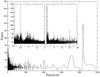 |
Fig. 6 Lomb-Scargle periodogram from the RV variations of HD 94660. |
Due to the limited temporal sampling of our dataset and the precision of our measurements, it is difficult to directly measure the expected RV differences from spectra taken on the same night. Therefore, it is not possible to verify the plausibility of the ~0.5 d period solution. However, as shown by Neiner et al. (2012), rapid RV variations that occur over the timescale of a single polarimetric sequence can induce detectable signatures in the diagnostic null profiles. These signatures result from residual polarisation signals that were not properly cancelled during processing because of the RV shifts. Therefore, the polarimetric spectra afford us the opportunity to test for the presence of short-period variations. To do so, we compared a synthetic model1, which takes into account the predicted RV variations according to the ~0.5 d period solution, to the mean LSD profiles extracted from the ESPaDOnS spectrum to test if null signatures should be present. The ESPaDOnS spectrum was obtained with the longest exposure time, and therefore should show the largest effect due to velocity shifts. Because of the strong polarisation signal, our results show that when RV shifts are added to each individual sub-exposure (in agreement with the expected variation suggested by short-period variations), the resulting null profile should also show a strong signature, which is easily detectable in the mean LSD profile. While this test cannot definitively rule out the possibility of short-term RV variations, it does provide compelling evidence against it. This result suggests that the ~0.5 d period is probably an alias of the correct period. We tested the plausibility of this hypothesis by subtracting a sinusoidal fit to the RV variations corresponding to the ~840 d period plus its first harmonic, and recomputed the periodogram on the residuals. The resulting periodogram no longer shows any significant power about 0.5 d, demonstrating it to be an alias of the ~840 d period.
Log of RV variations of HD 94660.
If the RVs do vary with the ~840 d period, it is our conclusion that these variations are likely the result of binarity. If these variations were due to shifts in the centre-of-gravity of the line profile due to the inhomogeneous surface distribution (e.g. spots) that is common among Ap/Bp stars, then we would expect much smaller RV shifts, which reflect the line distortion, with a maximum velocity range of the order of the line width. As well, we would expect periodicity consistent with the rotational period or one of its harmonics.
If we adopt this period as the orbital period then we obtain the orbital solution given in Table 7 using version 1.0.2 of the program Liège Orbital Solution Package (LOSP; Rauw et al., 2000). Figure 7 displays the RV orbital curve for this long period. Of particular interest, this solution suggests a high eccentricity ~0.4 and a high mass-function f(m) = m3sin3i/ (M + m)2 ~ 0.4 (where M is the mass of the observed star, m is the mass of the unseen companion and i is the orbital inclination). Using the 1σ limits of our estimated mass of HD 94660, this mass-function implies a lower mass limit for the companion of ≳2 M⊙. However, after co-aligning our spectra we find no evidence to suggest the presence of any additional spectral features that are not associated with HD 94660, which should be visible if HD 94660 hosted a ~2 M⊙ MS companion. Given the relatively high mass-function permitted by our preliminary orbital solution, the most likely candidate is a high-mass neutron star or black hole; however, further data is required to constrain the period and verify the orbital solution before any definitive conclusions can be made. Furthermore, our solution does not rule out the possibility of a hierarchical system, where the companion is a combination of several objects with a total combined mass of ≳2 M⊙ (such as two white dwarfs).
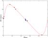 |
Fig. 7 Radial velocity orbital solution for the long 840 d period (dashed red line). Shown are the RV measurements for the HARPSpol (red squares), UVES (blue triangles) and ESPaDOnS (black dot) spectra. |
Preliminary orbital parameters for HD 94660.
8. Discussion and conclusions
HD 94660 is an Ap star commonly used as a magnetic standard for polarimetric observations in the southern hemisphere. It has an effective temperature Teff = 11 300 K with log L/L⊙ = 2.02 and mass M/M⊙ = 3.0. The rotation period is approximately 2800 d and vsini is less than about 2 km s-1. The surface magnetic field strength is of order 6 kG globally.
The aim of this project is to establish a preliminary magnetic field model of HD 94660 to use to estimate the atmospheric abundances of several chemical elements. The magnetic field model adopted is a simple, low-order axisymmetric multipole expansion whose parameters are established by fitting the observed periodic variations in ⟨ Bz ⟩ and ⟨ B ⟩ to computed models. This model is produced in the framework of the oblique rotator model and reasonably reproduces the observed variations in ⟨ Bz ⟩ and ⟨ B ⟩ with rotational phase (Fig. 1). The model is only a coarse approximation to the true field geometry of HD 94660, but is able to reproduce the observed Zeeman splitting and Stokes V signatures with rotational phase reasonably well (Fig. 3). This simple magnetic model is adequate to make it possible to determine a first approximation of the atmospheric abundances of this star. The actual parameters of this model are discussed in Sect. 4.3 and presented in Table 1.
We have used a dozen high-dispersion I spectra, well distributed in phase over the rotation cycle of the star, for a preliminary investigation of the surface chemistry and a characterisation of how the derived abundances may vary over the stellar surface. From the magnetic field model, the fact that i plus β is small (≲50°) indicates that we are mainly observing one magnetic hemisphere, with limited information about the opposite magnetic hemisphere. Although more than half of the stellar surface is seen, our investigations indicate very little abundance variations with rotational phase. For all elements studied, a single abundance fits well all available spectra and therefore a model with a uniform abundance distribution over the stellar surface is adopted.
As is expected for magnetic Ap stars, most elements studied have non-solar abundances. The abundances of O, Mg and Ca are all slightly below solar abundance ratios. Only an upper limit for He is possible which clearly classifies HD 94660 as He-weak, with a value at least 10 times less than the solar abundance. All other elements studied are more abundant than in the Sun. Most drastically, the rare-earth elements La, Ce, Pr and Nd are all between about 103 to 104 times more abundant than in the Sun. The abundances of Si, Sr and the Fe-peak elements Ti, Cr, Mn, Fe, Co and Ni are also larger than the solar abundance ratios (by factors of order 103 or less). Although no significant variations with co-latitude are observed in the stellar spectra, within a single spectrum the Fe-peak elements, calcium and silicon exhibit strong evidence of vertical stratification. This is most notable for Fe, where abundances derived from weak and strong lines of Fe ii (as well as weaker neutral Fe lines) differ by factors of order 10. Furthermore, the discrepant abundances derived from lines of Si ii and Si iii reported by Bailey & Landstreet (2013a) are also present in HD 94660. A more detailed analysis of abundance stratification in this star is clearly warranted. The discovery of Co in HD 94660 was surprising and further detailed studies of other hot magnetic Ap stars are recommended to ascertain the overabundance of this element in the atmospheres of these stars.
Landstreet et al. (2014) highlight the fact that HD 94660 is a star where there is poor agreement between the ⟨ Bz ⟩ measurements made from instruments with lower and higher resolutions. This is evident in Fig. 1 where the field strengths extracted from the HARPSpol and ESPaDOnS spectra using the entire metallic spectrum disagree with the FORS1 measurements. This phenomenon is also present in other stars such as HD 318107 (see Bailey et al., 2011), NGC 2169-12, NGC 2244-334 and HD 149277 (see Bagnulo et al., 2006). The disagreement between field measurements, using LSD, of different elements found in HD 94660 is also not uncommon (e.g. Manfroid & Mathys 2000; Bailey et al. 2011 for HD 318107 and Bailey et al. 2012 for HD 133880). These types of discrepancies are generally considered an indication of the inhomogeneous field distributions and large horizontal abundance variations (“spots”) on the stellar surface. This hypothesis is supported by more detailed maps of Ap stars using magnetic Doppler imaging (MDI) in which clear, complex field distributions and anomalous abundance spots are observed on the stellar surface (e.g. Kochukhov et al., 2004).
The RV variations measured in HD 94660 arise from orbital motion. Because of the long period currently favoured by the measurements (~840 d), this would suggest a massive compact companion such as a high-mass neutron star or black hole, or possibly a hierarchical system, where the companion is a combination of several objects with a total combined mass of ≳2 M⊙. It is rare for an A-type star to host a massive compact companion (see Kaper et al., 2006) and further monitoring is warranted to better constrain the properties of the companion. This system could help to establish the role that binarity may play in the origin of magnetism in stars with radiative envelopes (e.g. Grunhut & Alecian, 2014,and references therein).
HD 94660 is a star that warrants further investigation and highlights the need to study more sharp-lined magnetic stars in detail. Such studies are crucial to further understand the interplay between the magnetic field and the formation of vertical stratification in the atmospheres of Ap stars. They also provide important laboratories to test our multi-line techniques for measuring magnetic fields, such as LSD, by allowing measurements of magnetic field strengths from individual lines, a task that is not possible for stars that are fast rotators. At present, it is unclear what the discrepant field measurements for different lines of the same element are telling us about the chemical or magnetic structure of Ap stars, and therefore further analysis is required. Long term monitoring is also clearly indicated to firmly establish the nature of the RV variations observed in HD 94660.
This model is constructed by producing a sequence of individual synthetic sub-exposures with different RVs and treating them in the same fashion as the observations using the double-ratio method (Donati et al., 1997).
Acknowledgments
The authors thank Dr. Stephan Geier of ESO for helpful discussions. The authors also thank R.H.D. Townsend for the Lomb-Scargle code. J.D.L. acknowledges financial support from the Natural Sciences and Engineering Research Council of Canada. The authors also thank the referee Gautier Mathys for his comments that helped improve the manuscript.
References
- Asplund, M., Grevesse, N., Sauval, A. J., & Scott, P. 2009, ARA&A, 47, 481 [NASA ADS] [CrossRef] [Google Scholar]
- Babel, J. 1992, A&A, 258, 449 [NASA ADS] [Google Scholar]
- Bagnulo, S., Wade, G. A., Donati, J.-F., et al. 2001, A&A, 369, 889 [NASA ADS] [CrossRef] [EDP Sciences] [Google Scholar]
- Bagnulo, S., Landstreet, J. D., Mason, E., et al. 2006, A&A, 450, 777 [NASA ADS] [CrossRef] [EDP Sciences] [Google Scholar]
- Bailey, J. D. 2014, A&A, 568, A38 [NASA ADS] [CrossRef] [EDP Sciences] [Google Scholar]
- Bailey, J. D., & Landstreet, J. D. 2013a, A&A, 551, A30 [NASA ADS] [CrossRef] [EDP Sciences] [Google Scholar]
- Bailey, J. D., & Landstreet, J. D. 2013b, MNRAS, 432, 1687 [NASA ADS] [CrossRef] [Google Scholar]
- Bailey, J. D., Landstreet, J. D., Bagnulo, S., et al. 2011, A&A, 535, A25 [NASA ADS] [CrossRef] [EDP Sciences] [Google Scholar]
- Bailey, J. D., Grunhut, J., Shultz, M., et al. 2012, MNRAS, 423, 328 [NASA ADS] [CrossRef] [Google Scholar]
- Bailey, J. D., Landstreet, J. D., & Bagnulo, S. 2014, A&A, 561, A147 [NASA ADS] [CrossRef] [EDP Sciences] [Google Scholar]
- Bohlender, D. A., Landstreet, J. D., & Thompson, I. B. 1993, A&A, 269, 355 [NASA ADS] [CrossRef] [Google Scholar]
- Borra, E. F., & Landstreet, J. D. 1975, PASP, 87, 961 [NASA ADS] [CrossRef] [Google Scholar]
- Donati, J.-F., & Landstreet, J. D. 2009, ARA&A, 47, 333 [NASA ADS] [CrossRef] [MathSciNet] [Google Scholar]
- Donati, J.-F., Semel, M., Carter, B., Rees, D., & Collier Cameron, A. 1997, MNRAS, 291, 658 [NASA ADS] [CrossRef] [MathSciNet] [Google Scholar]
- Dworetsky, M. M., Trueman, M. R. G., & Stickland, D. J. 1980, A&A, 85, 138 [NASA ADS] [Google Scholar]
- Girardi, L., Bressan, A., Bertelli, G., & Chiosi, C. 2000, A&AS, 141, 371 [NASA ADS] [CrossRef] [EDP Sciences] [Google Scholar]
- Grunhut, J. H., & Alecian, E. 2014, IAU Symp., 302, 70 [NASA ADS] [Google Scholar]
- Hensberge, H. 1993, in Peculiar versus Normal Phenomena in A-type and Related Stars, IAU Colloq., 138, eds. M. M. Dworetsky, F. Castelli, & R. Faraggiana, ASP Conf. Ser., 44, 547 [Google Scholar]
- Kaper, L., van der Meer, A., van Kerkwijk, M., & van den Heuvel, E. 2006, The Messenger, 126, 27 [NASA ADS] [Google Scholar]
- Kochukhov, O., Bagnulo, S., Wade, G. A., et al. 2004, A&A, 414, 613 [NASA ADS] [CrossRef] [EDP Sciences] [Google Scholar]
- Kochukhov, O., Makaganiuk, V., & Piskunov, N. 2010, A&A, 524, A5 [NASA ADS] [CrossRef] [EDP Sciences] [Google Scholar]
- Kunzli, M., North, P., Kurucz, R. L., & Nicolet, B. 1997, A&AS, 122, 51 [NASA ADS] [CrossRef] [EDP Sciences] [Google Scholar]
- Kupka, F., Piskunov, N. E., Ryabchikova, T. A., Stempels, N. C., & Weiss, W. W. 1999, A&A, 138, 119 [Google Scholar]
- Kupka, F. G., Ryabchikova, T. A., Piskunov, N. E., Stempels, H. C., & Weiss, W. W. 2000, Balt. Astron., 9, 590 [NASA ADS] [Google Scholar]
- Landstreet, J. D. 1988, ApJ, 326, 967 [NASA ADS] [CrossRef] [Google Scholar]
- Landstreet, J. D., & Mathys, G. 2000, A&A, 359, 213 [NASA ADS] [Google Scholar]
- Landstreet, J. D., Bagnulo, S., Andretta, V., et al. 2007, A&A, 470, 685 [NASA ADS] [CrossRef] [EDP Sciences] [Google Scholar]
- Landstreet, J. D., Silaj, J., Andretta, V., et al. 2008, A&A, 481, 465 [NASA ADS] [CrossRef] [EDP Sciences] [Google Scholar]
- Landstreet, J. D., Bagnulo, S., & Fossati, L. 2014, A&A, 572, A113 [NASA ADS] [CrossRef] [EDP Sciences] [Google Scholar]
- Makaganiuk, V., Kochukhov, O., Piskunov, N., et al. 2011, A&A, 525, A97 [NASA ADS] [CrossRef] [EDP Sciences] [Google Scholar]
- Manfroid, J., & Mathys, G. 2000, A&A, 364, 689 [NASA ADS] [Google Scholar]
- Mathys, G. 1990, A&A, 232, 151 [NASA ADS] [Google Scholar]
- Mathys, G. 2013, in Progress in Physics of the Sun and Stars: A New Era in Helio- and Asteroseismology, eds. H. Shibahashi, & A. E. Lynas-Gray, ASP Conf. Ser., 479, 81 [Google Scholar]
- Mathys, G., & Hubrig, S. 1997, A&AS, 124, 475 [NASA ADS] [CrossRef] [EDP Sciences] [Google Scholar]
- Mathys, G., Hubrig, S., Landstreet, J. D., Lanz, T., & Manfroid, J. 1997, A&AS, 123, 353 [NASA ADS] [CrossRef] [EDP Sciences] [Google Scholar]
- Napiwotzki, R., Schoenberner, D., & Wenske, V. 1993, A&A, 268, 653 [NASA ADS] [Google Scholar]
- Neiner, C., Landstreet, J. D., Alecian, E., et al. 2012, A&A, 546, A44 [NASA ADS] [CrossRef] [EDP Sciences] [Google Scholar]
- Nesvacil, N., Shulyak, D., Ryabchikova, T. A., et al. 2013, A&A, 552, A28 [NASA ADS] [CrossRef] [EDP Sciences] [Google Scholar]
- Nielsen, K., & Wahlgren, G. M. 2000, A&A, 356, 146 [NASA ADS] [Google Scholar]
- Piskunov, N. E., & Valenti, J. A. 2002, A&A, 385, 1095 [NASA ADS] [CrossRef] [EDP Sciences] [Google Scholar]
- Piskunov, N. E., Kupka, F., Ryabchikova, T. A., Weiss, W. W., & Jeffery, C. S. 1995, A&A, 112, 525 [Google Scholar]
- Piskunov, N., Snik, F., Dolgopolov, A., et al. 2011, The Messenger, 143, 7 [NASA ADS] [Google Scholar]
- Press, W., Teukolsky, S., Vetterling, W., & Flannery, B. 1992, Numerical recipes in FORTRAN. The art of scientific computing (Cambridge: Cambridge University Press) [Google Scholar]
- Rauw, G., Sana, H., Gosset, E., et al. 2000, A&A, 360, 1003 [NASA ADS] [Google Scholar]
- Rees, D., & Semel, M. 1979, A&A, 74, 1 [NASA ADS] [Google Scholar]
- Renson, P., Gerbaldi, M., & Catalano, F. A. 1991, A&AS, 89, 429 [NASA ADS] [Google Scholar]
- Rusomarov, N., Kochukhov, O., Piskunov, N., et al. 2013, A&A, 558, A8 [NASA ADS] [CrossRef] [EDP Sciences] [Google Scholar]
- Ryabchikova, T. A. 1991, in Evolution of Stars: the Photospheric Abundance Connection, eds. G. Michaud, & A. V. Tutukov, IAU Symp., 145, 149 [Google Scholar]
- Ryabchikova, T. A., Piskunov, N. E., Kupka, F., & Weiss, W. W. 1997, Balt. Astron., 6, 244 [NASA ADS] [Google Scholar]
- Stibbs, D. W. N. 1950, MNRAS, 110, 395 [NASA ADS] [CrossRef] [Google Scholar]
- van Leeuwen, F. 2007, A&A, 474, 653 [NASA ADS] [CrossRef] [EDP Sciences] [Google Scholar]
- Wade, G. A., Donati, J.-F., Landstreet, J. D., & Shorlin, S. L. S. 2000, MNRAS, 313, 823 [NASA ADS] [CrossRef] [MathSciNet] [Google Scholar]
All Tables
The abundances are measured with respect to H, and are tabulated with their associated uncertainties.
All Figures
|
Fig. 1 ⟨ Bz ⟩ and ⟨ B ⟩ variations of HD 94660. The solid black lines are the adopted magnetic field model variations from Sect. 4.3. Top: ⟨ Bz ⟩ LSD measurements using the full mask (black circles) and Nd mask (green triangles). Note that the open and filled symbols denote measurements from the ESPaDOnS spectrum and HARPSpol spectra, respectively. Balmer line measurements from Landstreet et al. (2014) are the filled red squares. Bottom: phased ⟨ B ⟩ measurements from Fe ii 6149 (blue squares), Cr ii 6833 (red triangles) and Nd iii 6145 (green circles). The dotted green line is the best-fit sinusoidal variations to the Nd measurements. |
| In the text | |
|
Fig. 2 Variations in magnetic field strength ⟨ Bz ⟩ versus EQW for individual spectral lines. Different symbols denote different elements, while different colours are used to represent different Landé factor ranges. Note that the absolute value of the field strength is shown and each measurement has been normalised as discussed in the text. The dashed line is a linear fit to the data. |
| In the text | |
|
Fig. 3 A comparison of magnetic field models. In black are the observed Stokes I (top) and V (bottom) profiles for Nd iii λ6145 for the 28-08-2014 HARPSpol spectrum. We overplot the computed line profiles for our adopted magnetic field geometry (red dashed line) and the magnetic field geometry of Landstreet & Mathys (2000; blue dotted line). |
| In the text | |
|
Fig. 4 A comparison of the Stokes Q signatures of synthetic models to the HARPSpol observation on 01-04-2012. In black is the observed Stokes Q spectrum. Overplotted is our adopted magnetic field model (red dashed line). The top panel assumes i>β, whereas the bottom assumes i<β. |
| In the text | |
|
Fig. 5 Example of three synthesised spectral windows for the 28-04-2014 HARPSpol spectrum of HD 94660. The observed spectrum is in black (solid line) and the model is in red (dashed line). The bottom panel illustrates the vertical stratification of Fe in the atmosphere of HD 94660, where strong lines of Fe ii and weak lines of Fe i are fit well with the abundance of Table 5, but the weaker lines of Fe ii require an enhanced abundance to be well modelled. |
| In the text | |
|
Fig. 6 Lomb-Scargle periodogram from the RV variations of HD 94660. |
| In the text | |
|
Fig. 7 Radial velocity orbital solution for the long 840 d period (dashed red line). Shown are the RV measurements for the HARPSpol (red squares), UVES (blue triangles) and ESPaDOnS (black dot) spectra. |
| In the text | |
Current usage metrics show cumulative count of Article Views (full-text article views including HTML views, PDF and ePub downloads, according to the available data) and Abstracts Views on Vision4Press platform.
Data correspond to usage on the plateform after 2015. The current usage metrics is available 48-96 hours after online publication and is updated daily on week days.
Initial download of the metrics may take a while.