| Issue |
A&A
Volume 575, March 2015
|
|
|---|---|---|
| Article Number | A12 | |
| Number of page(s) | 20 | |
| Section | Stellar structure and evolution | |
| DOI | https://doi.org/10.1051/0004-6361/201424686 | |
| Published online | 11 February 2015 | |
Uncertainties in asteroseismic grid-based estimates of stellar ages
SCEPtER: Stellar CharactEristics Pisa Estimation gRid⋆
1
INAF – Osservatorio Astronomico di Collurania, via Maggini,
64100
Teramo,
Italy
e-mail:
valle@df.unipi.it
2
INFN, Sezione di Pisa, Largo Pontecorvo 3,
56127
Pisa,
Italy
3
Dipartimento di Fisica “Enrico Fermi”, Università di
Pisa, Largo Pontecorvo
3, 56127
Pisa,
Italy
Received: 26 July 2014
Accepted: 8 December 2014
Context. Stellar age determination by means of grid-based techniques that adopt asteroseismic constraints is a well established method nowadays. However some theoretical aspects of the systematic and statistical errors affecting these age estimates still have to be investigated.
Aims. We study the impact on stellar age determination of the uncertainty in the radiative opacity, in the initial helium abundance, in the mixing-length value, in the convective core overshooting, and in the microscopic diffusion efficiency adopted in stellar model computations.
Methods. We extended our SCEPtER grid to include stars with mass in the range [0.8; 1.6] M⊙ and evolutionary stages from the zero-age main sequence to the central hydrogen depletion. For the age estimation we adopted the same maximum likelihood technique as described in our previous work. To quantify the systematic errors arising from the current uncertainty in model computations, many synthetic grids of stellar models with perturbed input were adopted.
Results. We found that the current typical uncertainty in the observations accounts for 1σ statistical relative error in age determination, which on average ranges from about −35% to +42%, depending on the mass. However, owing to the strong dependence on the evolutionary phase, the age’s relative error can be higher than 120% for stars near the zero-age main sequence, while it is typically of the order of 20% or lower in the advanced main-sequence phase. The systematic bias on age determination due to a variation of ±1 in the helium-to-metal enrichment ratio ΔY/ΔZ is about one-fourth of the statistical error in the first 30% of the evolution, while it is negligible for more evolved stages. The maximum bias due to the presence of the convective core overshooting is −7% and −13% for mild and strong overshooting scenarios. For all the examined models, the impact of a variation of ±5% in the radiative opacity was found to be negligible. The most important source of bias is the uncertainty in the mixing-length value αml and the neglect of microscopic diffusion. Each of these effects accounts for a bias that is nearly equal to the random error uncertainty. Comparison of the results of our technique with other grid techniques on a set of common stars showed general agreement. However, the adoption of a different grid can account for a variation in the mean estimated age up to 1 Gyr.
Key words: methods: statistical / stars: evolution / stars: oscillations / stars: low-mass / stars: fundamental parameters / asteroseismology
Appendices are available in electronic form at http://www.aanda.org
© ESO, 2015
1. Introduction
The determination of stellar ages cannot be obtained by direct measurements; therefore, several techniques – with different ranges of applicability – have been developed to obtain reasonable age estimates (see Soderblom 2010, for a review). Traditionally, the age estimate for a main-sequence single star involves either the use of a rotation-mass-age relationship or the comparison of computed isochrones to observed parameters, which are classically magnitudes, colours, and metallicity. It is, however, well known that the precision of these estimates is unsatisfactory (see e.g. Lebreton & Montalbán 2009; Lebreton 2013; Epstein & Pinsonneault 2014, and references therein).
The availability of high-quality data from asteroseismology satellite missions, such as CoRoT (see e.g. Appourchaux et al. 2008; Michel et al. 2008; Baglin et al. 2009) and Kepler (see e.g. Borucki et al. 2010; Gilliland et al. 2010), has offered a strong contribution to stellar age estimation. These data, combined with the traditional ones, increase the constraints on the theoretical models, thereby allowing significant improvement.
It has recently been shown that the single-star modelling in the presence of individual frequencies of the oscillation spectrum can provide age estimates that are more precise than 15%, with a typical factor of two improvements over grid-based estimates when adopting the average large frequency spacing Δν and the frequency of maximum oscillation power νmax as seismic observables (Lebreton 2013; Silva Aguirre et al. 2013; Metcalfe et al. 2014). However, these techniques are computationally intensive and are restricted only to stars for which high signal-to-noise data are available. The alternative approach based on grid techniques adopting Δν and νmax (see e.g. Stello et al. 2009; Basu et al. 2010; Quirion et al. 2010; Gai et al. 2011; Huber et al. 2013) has been recognized to allow a fast and automated way to obtain stellar ages from data. Although several studies have been devoted to quantifying the uncertainty affecting these grid-based estimates (see e.g. Gai et al. 2011; Lebreton 2013) a comprehensive examination of the various bias sources and statistical uncertainties is still lacking. In this paper we continue the work started in Valle et al. (2014, hereafter V14) – focused on mass and radius estimates – by exploring the systematic biases on grid-based age estimates due to the uncertainties on the main error sources in theoretical predictions: the radiative opacity, the microscopic diffusion efficiency, the mixing-length parameter value, the initial helium abundance-metallicity relationship, and convective core overshooting extension. We restrict our analysis to central hydrogen-burning stars with mass in the range [0.8; 1.6] M⊙.
The structure of the paper is the following. In Sect. 2 we discuss the method and the grids used in the estimation process. The main results are presented in Sects. 3 and 4. Section 5 presents a comparison of the estimates obtained with our grids with those by other grid-based techniques. Some concluding remarks can be found in Sect. 6.
2. Grid-based recovery technique
We adopted the SCEPtER scheme1 described in V14 and derived from Basu et al. (2012). For reader’s convenience we summarize the basic aspects of the procedure. We let  be a star for which the following vector of observed quantities is available:
 ![\hbox{$q^{\cal S} \equiv \{T_{\rm eff, \cal S}, {\rm [Fe/H]}_{\cal S}, \Delta \nu_{\cal S}, \nu_{\rm max, \cal S}\}$}](/articles/aa/full_html/2015/03/aa24686-14/aa24686-14-eq14.png) . Then we let
. Then we let ![\hbox{$\sigma = \{\sigma(T_{\rm eff, \cal S}), \sigma({\rm [Fe/H]}_{\cal S}), \sigma(\Delta \nu_{\cal S}), \sigma(\nu_{\rm max, \cal S})\}$}](/articles/aa/full_html/2015/03/aa24686-14/aa24686-14-eq15.png) be the nominal uncertainty in the observed quantities. For each point j on the estimation grid of stellar models, we define qj ≡ { Teff,j, [ Fe/H ] j,Δνj,νmax,j }. We let ℒj be the likelihood function defined as
be the nominal uncertainty in the observed quantities. For each point j on the estimation grid of stellar models, we define qj ≡ { Teff,j, [ Fe/H ] j,Δνj,νmax,j }. We let ℒj be the likelihood function defined as  (1)where
  (2)The likelihood function is evaluated for each grid point within 3σ of all the variables from . We let ℒmax be the maximum value obtained in this step. The estimated stellar mass, radius, and age are obtained by averaging the corresponding quantity of all the models with likelihood greater than 0.95 × ℒmax. Informative priors can be inserted as a multiplicative factor in Eq. (1), as a weight attached to the grid points.
The technique can also be employed to construct a Monte Carlo confidence interval for mass, radius, and age estimates. To this purpose a synthetic sample of n stars is generated, following a multivariate normal distribution with vector of mean  and covariance matrix Σ = diag(σ). A value of n = 10 000 is usually adopted since it provides a fair balance between computation time and the accuracy of the results. The medians of the n objects mass, radius, and age are taken as the best estimate of the true values; the 16th and 84th quantiles of the n values are adopted as a 1σ confidence interval.
2.1. Standard stellar models grid
The standard estimation grid of stellar models is obtained using FRANEC stellar evolution code (Degl’Innocenti et al. 2008), in the same configuration as was adopted to compute the Pisa Stellar Evolution Data Base2 for low-mass stars (Dell’Omodarme et al. 2012; Dell’Omodarme & Valle 2013).
The grid consists of 141 680 points (110 points for 1288 evolutionary tracks), corresponding to evolutionary stages from the zero-age main sequence (ZAMS) to central hydrogen depletion. Models are computed for masses in the range [0.80; 1.60] M⊙ with a step of 0.01 M⊙. The initial metallicity [Fe/H] is assumed in the range [−0.55; 0.55] with a step of 0.05 dex. The solar-scaled heavy-element mixture by Asplund et al. (2009) is adopted. The initial helium abundance is obtained using the linear relation  adopting a primordial 4He abundance value Yp = 0.2485 from WMAP (Cyburt et al. 2004; Steigman 2006; Peimbert et al. 2007a,b), and assuming ΔY/ΔZ = 2 (Pagel & Portinari 1998; Jimenez et al. 2003; Gennaro et al. 2010). The models are computed assuming our solar-scaled mixing-length parameter αml = 1.74. Convective core overshooting is not taken into account. Atomic diffusion is included adopting the coefficients given by Thoul et al. (1994) for gravitational settling and thermal diffusion. To prevent the surface helium and metal depletion for stars without a convective envelope, a diffusion inhibition mechanism similar to the one discussed in Chaboyer et al. (2001) is considered. For the outermost 1% in mass of the star, the diffusion velocities are multiplied by a suppression parabolic factor that takes value 1 at the 99% in mass of the structure and 0 at the base of the atmosphere. Further details on the input adopted in the computations are available in Valle et al. (2014, 2009).
As in V14, the average large frequency spacing Δν and the frequency of maximum oscillation power νmax are obtained using a simple scaling from the solar values (Ulrich 1986; Kjeldsen & Bedding 1995): 
 |
Fig. 1 Age estimate relative errors as a function of the true mass (left panel), relative age (central panel), and metallicity [Fe/H] (right panel) of the star. The blue long dashed lines mark the error medians. The red solid line is the 1σ error envelope, while the red dashed one marks the position of the 2σ envelope (see text). A positive relative error indicates that the reconstructed age of the star is overestimated with respect to the true one. |
3. Age estimates: grid technique internal accuracy
The age recovery procedure was first tested on a synthetic dataset obtained by sampling N = 50 000 artificial stars from the same standard estimation grid of stellar models used in the recovery procedure itself and adding a Gaussian noise in all the observed quantities to each of them. As in V14, we adopted the same standard deviation values suggested by Gai et al. (2011): i.e. 2.5% in Δν, 5% in νmax, 100 K in Teff, and 0.1 dex in [Fe/H].
For each synthetic star, the relative error on the reconstructed age was computed. A positive relative error indicates that the age of the star is overestimated by the recovery procedure. Figure 1 shows the trend of the age relative errors versus the true mass of the star, its relative age – conventionally set to 0 at the ZAMS position and defined as the ratio between the current age of the star and its age at the central hydrogen depletion – and its metallicity [Fe/H]3. The figure also shows the relative error envelopes obtained by evaluating the 16th and 84th quantiles (1σ) and 2.5th and 97.5th quantiles (2σ) of the age relative error over a moving window4. The position of the 1σ envelope and of the median of the age relative error in dependence on the true mass of the star and on its relative age are reported in Tables 1 and 2, in the section labelled “standard”.
As expected and already reported in literature (see e.g. Gai et al. 2011; Chaplin et al. 2014), age determinations are much less constrained than mass and radius ones. Moreover, the distribution of relative errors on age estimates is typically asymmetric and present a long tail toward age overestimate. This is due to the presence of the hard boundary at −1.0 since age estimates can not be negative.
Both the plot of the age relative errors versus the mass of the star and Table 1 show that the overall 1σ envelope ranges from about −35% to +42%. Moreover, it is evident the presence of an “edge effect” similar to that extensively discussed in V14. At the lower edge of the grid (M = 0.80 M⊙), the age of the stars are biased towards low values, while the opposite occurs at the upper edge (M = 1.60 M⊙). This trend is easily understood considering that a star with M = 0.80 M⊙ can be confused in the recovery with a slightly more massive model, which evolves faster and thus has a lower age, while no models at lower mass, and therefore older, exist in the grid.
The central panel in Fig. 1 and Table 2 show the strong dependence of the age relative error on the evolutionary phase: the closer the star is to the ZAMS and the larger the uncertainty. The age relative error can be higher than 120% near the ZAMS, while it is typically of the order of 20% or lower in the advanced main-sequence phase. The high value of the upper envelope border at low relative age is not surprising since an error on age estimates has a strong impact here since stellar ages are low. The envelope is highly asymmetric since, at low relative ages, the grid edge limits the possibility of age underestimation, thus resulting in biased estimates. In other words, approaching the ZAMS, grid-based age estimates not only become considerably more uncertain but also biased towards older ages. The increase in the relative age leads to a shrinking of the age-relative error envelope. A small envelope inflation is present around the relative age 0.8, which is due to the presence of a convective core for the more massive models (see Sect. 4.4); at a relative age higher than about 0.85 the envelope shows a shrinking, because age estimations are intrinsically easier in rapidly evolving phases (see e.g. the results in Gai et al. 2011; Chaplin et al. 2014).
The trend versus [Fe/H] stems from the trend in relative age and from edge effects. The envelope of the relative error is narrower for [Fe/H] lower than about −0.8 dex, since for these values only evolved models (relative age of about 0.8) are present. These models reach such a low surface metallicity due to microscopic diffusion (we recall that the lowest initial metallicity in the grid is [Fe/H] = −0.55 dex), which takes long time scales to produce observable effects. In contrast, at the upper metallicity edge, there must only be models young enough for diffusion to be inefficient, i.e. models at very early evolutionary stages, and consequently age estimates get less precise, leading to a larger envelope.
SCEPtER median (q50) and 1σ envelope boundaries (q16 and q84) for age relative error as a function of the mass of the star.
SCEPtER median (q50) and 1σ envelope boundaries (q16 and q84) for age relative error as a function of the relative age of the star.
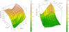 |
Fig. 2 Left: lower boundary of the 2D envelope of age estimate relative errors as a function of mass and relative age of the star. Right: same as in the left panel, but for the upper envelope boundary. |
The medians (q50) in the tables clearly show the presence of the edge effect distortions discussed above. Figure 1 allows the position of the 1σ envelope boundary to be assessed as a function of the mass of the star disregarding the relative ages or as a function of the stellar relative age disregarding the masses. To show how the mass and the relative age jointly influence the boundary of the envelope, a 2D envelope was computed with a bidimensional generalization of the technique described above5. The left-hand panel of Fig. 2 shows the position of the lower boundary 2D envelope, while the upper one is in the right-hand panel. Several aspects discussed above are clearly visible, such as the edge effect at low mass (right panel) and low relative ages where we note the lack of models with overestimated age; this causes the strong decrease of the envelope in this region. The lower envelope boundary (left panel) shows a little decrease at about 1.3 M⊙ at a relative age greater than about 0.8. This effect is caused by the presence of a convective core for stars more massive than about 1.1 M⊙, which modifies the morphology of the stellar track and its evolutionary time scale. The consequence is a displacement on the grid towards models of different masses and ages. In particular, the relative age difference of the models around 1.3 M⊙ has a lower 16th quantile than less massive models. For target of about 1.5 M⊙, an edge effect masks the shift of the quantile since higher mass and lower age models are under-represented in the neighbourhood of the target point.
The results presented above can be compared with those of a similar analysis conducted by Gai et al. (2011). The relative error in age estimates are analysed in that paper, which assumes the same uncertainties in the observational constraints adopted here. The results are presented as a histogram, and the half-width at half-maximum (HWHM) is adopted to describe the spread of the distribution. An overall HWHM of about 15% is reported in Gai et al. (2011). For comparison, we computed a kernel density estimate (see Scott 1992; Venables & Ripley 2002, and the Appendix A in Valle et al. 2014) for our results founding an HWHM of about 20%. A comparison of the two numbers should take into account that the grid used in Gai et al. (2011) covers a different range of masses (up to 3.0 M⊙) and includes red giants models. Moreover, Fig. 23 by Gai et al. (2011) shows a variation in the HWHM according to the evolutionary phase of the stars: stars in the earlier stages of evolution have a HWHM of their relative error histogram much larger than evolved stars. This is the same qualitative trend that we analysed in detail and quantitatively report in Table 2.
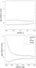 |
Fig. 3 Envelope of age-estimate relative errors as a function of mass and relative age of the star for different assumptions on the observational errors. The solid line corresponds to the standard case; the dashed one to σ(Teff) = 50 K; the dotted one to σ( [ Fe/H ] ) = 0.05 dex; the dot-dashed one to σ(Δν) = 1%, σ(νmax) = 2.5%. |
3.1. Impact of the observational errors and mass-age correlation
To explore the sensitivity of the uncertainty on grid-technique age estimates to the precision of the data, we repeated the procedure by varying the observational uncertainties. In this test we halved one uncertainty at a time, while keeping the uncertainties in the other quantities fixed to the standard value. The first test assumes 50 K as Teff error, the second test adopts an uncertainty of 0.05 dex in [Fe/H], while the last one assumes an uncertainty of 1% in Δν and 2.5% in νmax. The results are presented in Fig. 3 and in Tables 1 and 2 in the sections labelled “σ(Teff) = 50 K”, “σ( [ Fe/H ] ) = 0.05 dex”, and “σ(Δν,νmax) = 1%, 2.5%”.
Observing the shrink of the relative error on age estimates envelopes, it is apparent that the refinement of Teff determination is the most important factor for stars of mass lower than about 1.2 M⊙, while for more massive objects the metallicity and asteroseismic refinement have more importance. The reduction of the single-source observational uncertainties have a maximum impact of about 10% in the absolute shrink, which is about one-third of the reference envelope half width. Regarding the error envelope in dependence on relative age, for relative ages lower than about 0.4 the seismic refinement causes the greater shrinkage of the envelope, while at later evolutionary stages, the effective temperature refinement is the most important factor.
The errors on mass and age estimates are expected to show a negative trend, because a star can be confused in the recovery procedure either with a higher mass and lower age model or with a lower mass and higher age one (see e.g. Fig. 4 in V14). It also follows from the discussion in V14 that the strength of the linear correlation between mass and age relative errors is expected to increase with the relative age of the star. This trend is shown in Fig. 4, which shows the dependence of relative errors on mass and age estimates, grouped in three relative age classes: models with relative age lower than 0.2; models with relative ages between 0.2 and 0.4; models with relative age greater than 0.4. The decrease in the slope of age versus mass relative errors with the increase in relative age is due to the mild increase in mass estimates variance at the higher relative age that is extensively discussed in V14, and the corresponding strong decrease in variance in age estimates reported above. The correlation coefficient (a measure of the dispersion of the data around the ideal linear fit) between age and mass relative error in the three relative age groups are respectively −0.729 (95% confidence interval [−0.740; −0.718]), −0.906 (95% confidence interval [−0.910; −0.902]), and −0.922 (95% confidence interval [−0.924; −0.921]). Estimated ages can never be negative so the figure clearly shows the presence of a hard boundary at −1.0 for age relative error.
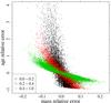 |
Fig. 4 Correlation between age and mass relative errors. The black circles correspond to models with relative age in the range [0.0; 0.2], the red triangles to relative ages in the range [0.2; 0.4], and the green crosses to relative ages in the range [0.4; 1.0]. |
3.2. Impact of weighting the estimation grid
As a last check on the standard grid, we verified the influence of taking the evolutionary time scale into account in the grid-based age estimation. In fact, the grids of stellar models are biased towards rapid evolving stages, where more points are computed to accurately follow the evolution. It is well known that neglecting this effect can lead to significantly biased estimates (see e.g. Jørgensen & Lindegren 2005; Pont & Eyer 2004; Casagrande et al. 2011). To quantify this effect, we repeated the estimates described before for the same sample used in Sect. 3, which was obtained sampling from the grid without taking the evolutionary time scale into account, but by recovering ages adopting the corresponding evolutionary time scale as a weight of each grid point. The results are summarized in Tables 1 and 2, in the section labelled “weighted” and in Fig. 5. It appears that weighted estimates are slightly biased (q50 about 3%) towards higher ages than those obtained by adopting the standard grid for stars of mass lower than about 1.1 M⊙, while the opposite (q50 about −3%) occurs at higher masses. The same phenomenon occurs in dependence on relative age with an age overestimation at lower relative ages and an underestimation at high relative ages. These biases are smaller than the envelope width owing to random errors.
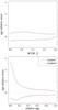 |
Fig. 5 Same as in Fig. 3, but for the comparison of standard and weighted estimates (see text for details). |
The weights cause a slight underestimation of the mass for stars less massive than about 1.1 M⊙, and a more pronounced overestimation for objects at about 1.4 M⊙. For low-mass stars, whose tracks evolve nearly parallel in the (Teff, Δν) plane, the weights have the strongest influence in the first stages of stellar evolution, until about relative age 0.6, where the differences in time scales amongst models of different mass become smaller.
In contrast, for more massive stars the overestimation in mass is due to the tracks crossing during the overall contraction phase. At the crossing, the time scale of the model of lower mass is shorter than that of the more massive one, and therefore the weighting estimates are biased towards a lower age. Figure 6 illustrates the effect showing the 1σ envelopes for mass relative error with respect to the mass of the star for standard and weighted estimates. The bias occurring at high mass is apparent.
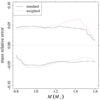 |
Fig. 6 Envelope of the mass relative error for stars sampled and reconstructed on the standard grid (black solid line), and for the same sample reconstructed on the weighted grid (red dashed line). |
In this section we have focused on the relative bias of the weighted age estimates with respect to the standard one, considering weights only in the recovery stage. This quantified a maximum possible distortion of the unweighted estimates with respect to the weighted one. It seems that in the presence of asteroseismic constraints weighted estimates of mass presents a bias, especially for massive models, not present in the unweigthed approach. Moreover, the differences in age estimates due to the grid weighting are much smaller than the random 1σ envelope half width. Therefore in the following we adopt unweighted estimates as our reference scenario when studying the effect of varied input in the stellar evolutionary computations. We instead adopt weighted estimates in Sect. 5 when comparing with other pipelines that actually take such a correction into account.
4. Stellar model uncertainty propagation
When grid-based techniques are applied to real stars rather than to synthetic ones, the accuracy and precision of age estimates depend on the goodness of the adopted stellar models. A change within the uncertainties of the input adopted in stellar evolutionary codes directly propagates into a variation in the grid-based results. In V14, we discussed extensively this issue for mass and radius estimates. Here we perform a similar analysis for age estimates. We focus our analysis on radiative opacity uncertainty, on the value of the mixing-length parameter, on the initial helium abundance, on the extension of any additional mixing region starting from the border of the convective zones defined by the Schwarzchild criterion, and on the efficiency of element diffusion.
We performed these estimates following V14. More in detail, for each of the previously mentioned input, we computed two non-standard grids of perturbed stellar models by varying the chosen individual input to its extreme values, while keeping all the others fixed to their reference values. Artificial stars are then sampled from these grids, and their ages are estimated on the standard one. As in V14, we followed a slightly different procedure to study the effect of diffusion.
The analysis of the difference between reconstructed and true values will quantitatively assess the effect of the quoted sources of uncertainties affecting modern stellar models. In general, perturbing a stellar model input leads to a twofold effect on the artificial stars. First, a displacement in the 4D space of the observational parameters (i.e. Teff, [ Fe/H ] ,Δν,νmax) with respect to the location of standard models of the same mass and age. Second, a variation in the evolutionary time scale. As detailed in the following, there are cases in which the two effects are opposite and have the same order of magnitude thus resulting in a small net bias. In others, the latter effect is negligible and no compensation occurs, leading to a large bias.
Given the strong dependence on the evolutionary phase of the age relative error, the bias at a given relative age must always be compared with the 1σ envelope at the same phase to assess the relevance of the bias itself.
4.1. Initial helium abundance
The helium-to-metal enrichment ratio ΔY/ΔZ, which is commonly adopted by stellar modellers to select the initial helium abundance, is quite uncertain (Pagel & Portinari 1998; Jimenez et al. 2003; Gennaro et al. 2010). To quantify the impact of such an uncertainty on grid-based age estimates, we computed two additional grids of stellar models with the same values of the metallicity Z as in the standard grid, but by changing the helium-to-metal enrichment ratio ΔY/ΔZ to values 1 and 3. Then, we built two synthetic datasets, each of N = 50 000 artificial stars, by sampling the objects from these two non-standard grids. The age of the objects was then estimated using the standard grid for the recovery.
The results of these tests are presented in sections “ΔY/ΔZ = 1” and “ΔY/ΔZ = 3” of Tables 1 and 2 and in the left-hand column of Fig. 7. The effect of the initial helium content change is modest on average. For ΔY/ΔZ = 1, a bias with respect to a standard case median of about 3% to 5% occurs for stellar masses below 1.1 M⊙, with a similar effect on the envelope boundaries. For ΔY/ΔZ = 3, the bias ranges from about −2% to −5% for stellar masses below 1.1 M⊙, with an envelope shift from about −7% to −10%. The strongest bias with respect to standard scenario results occurs at low relative age where it reaches values of about 21% and −25% for ΔY/ΔZ = 1 and 3.
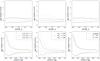 |
Fig. 7 Left column: envelopes of age estimate relative errors due to sampling from synthetic grids with different values of ΔY/ΔZ. Ages are estimated on the standard grid with ΔY/ΔZ = 2. Middle column: same as the left column, but for sampling from synthetic grids with different values of the mixing-length parameter αml. Ages are estimated on the standard grid with αml = 1.74. Right column: same as the left column, but for sampling from synthetic grids with different values of radiative opacity kr. Ages are estimated on the standard grid. |
As shown in V14, the strongest impact of the initial helium change occurs, as expected, for high values of [Fe/H]. To illustrate this point, let us consider the sampling from the grid with ΔY/ΔZ = 1 and the reconstruction on the standard grid (ΔY/ΔZ = 2). For stars on the upper metallicity edge, the effect of helium change is relevant. Figure 8 shows the age-relative error envelope for the considered values of helium-to-metal enrichment ratio as a function of the surface [Fe/H] value. It is apparent that the low helium scenario presents a very long tail towards age overestimation near [Fe/H] = 0.50 dex. This is because, for [Fe/H] values near the edge boundary, the ΔY/ΔZ = 1 models are significantly shifted towards higher asteroseismic parameters. As a consequence they are often confused in the recovery with standard near ZAMS models whose age is more difficult to estimate.
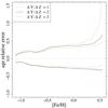 |
Fig. 8 Dependence on the surface metallicity [Fe/H] of the envelopes of age estimate relative errors. The sampling occurs from synthetic grids with different values of ΔY/ΔZ, while ages are estimated on the standard grid with ΔY/ΔZ = 2. |
The overall smallness of the effect of an helium abundance change might be unexpected since the initial helium content significantly affects the evolutionary time scale of stellar models. Moreover, in V14 we showed that the same variation in ΔY/ΔZ results in a sizeable uncertainty in the grid-based recovery of M and R. This effect is also confirmed for the masses up to 1.6 M⊙ studied here. The results are due to the concurrent change in the effective temperature and seismic parameters. This effect is shown in Fig. 9, which reports the boxplots of the differences in effective temperature and age for stellar models of same relative age computed with standard and varied input6. To enhance the figure readability, the outliers, which can be presented as individual points, are omitted from the plot. The medians shift are related to the effect of the input variation in the stellar evolutionary code. The larger the separation of the medians with respect to the interquartile distance of the boxes, the greater the importance of a given input variation.
It is apparent that a change in the initial helium content has a notable effect on both ages and effective temperature variations and that such variations partially counterbalance each other. As discussed in V14, an artificial star with enriched initial helium will have – at fixed evolutionary phase – a higher effective temperature and a lower age than the corresponding model of the same mass but computed with standard initial helium abundance. The change in the observational parameters forces the helium-rich star to lie in a zone of the standard grid populated by more massive models, leading to a mass overestimate in the recovery. However, helium-rich stars evolve faster than corresponding standard scenario stars. It happens that the age bias due to the mass overestimate nearly compensates for the difference in age due to the change in the initial helium, thus resulting in a small net bias in estimated age. It is also apparent that the balancing effect is more accurate for massive models and for later evolutionary stages, when the error envelopes computed with modified initial helium abundance converge to the standard one.
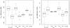 |
Fig. 9 Left: boxplots of the difference in effective temperature between standard models and models with varied input or parameters. The differences have been computed for models in the same evolutionary phase. A positive value implies that the standard grid provides an higher effective temperature. Right: same as the left panel, but for age. |
4.2. Mixing-length value
It is increasingly apparent that the use of a solar-calibrated mixing-length value for stars that differ from the Sun in mass, composition, and/or evolutionary phase could not be appropriate (see e.g. Deheuvels & Michel 2011; Bonaca et al. 2012; Mathur et al. 2012; Tanner et al. 2014; Trampedach & Stein 2011; Magic et al. 2015; Yıldız 2007; Clausen et al. 2009). To quantify the effect of varying the efficiency of the super-adiabatic convective transport, we computed two additional grids of stellar models by assuming mixing-length parameters αml = 1.50 and 1.98. Then, we built two synthetic datasets, each of N = 50 000 artificial stars, by sampling the objects from these two non-standard grids. The age of the objects are estimated using the standard grid for the recovery, which assumes our solar-calibrated value αml = 1.74. The results of these tests are presented in sections “αml = 1.50” and “αml = 1.98” of Tables 1 and 2 and in the central column of Fig. 7.
In this case the bias is very strong with values ranging from 20% to 30% for models of mass lower than 1.2 M⊙. As expected, the bias is lower for higher mass models owing to the decreasing thickness of the convective envelope. The bias due to the mixing-length variation is nearly the same as the 1σ random uncertainty of the standard models, implying that the age estimates are prone to systematic biases because of adoption of an improper mixing-length value. The origin of this large bias can be understood with the same argument discussed for initial helium content. Artificial stars with varied αml occupy a different location in the 4D space of the observable quantities with respect to standard models of the same mass and age. Consequently the recovered mass and age on the standard grid will be necessarily biased. Moreover, unlike the case of a variation in the helium abundance, changing the mixing-length does not affect the evolutionary time scale (see the boxplots in Fig. 9). As a result, the counterbalancing effect previously described in Sect. 4.1 cannot occur, and the age bias is large.
4.3. Radiative opacity
In Valle et al. (2013a,b), we made a strong computational effort to quantify the cumulative uncertainty affecting stellar models due to the combined effects of the main input physics. As a result we found that the main source of variation is due to the current uncertainty in the radiative opacities.
To quantify the impact of this uncertainty source on age estimates, we computed two additional grids with values of radiative opacity increased and decreased by 5% (see the discussion in Valle et al. 2013a, for the choice of the quoted uncertainty). Then, we built two synthetic datasets, each of N = 50 000 artificial stars, by sampling the objects from these two non-standard grids. The age of the objects are then estimated using the standard grid for the recovery.
The results of these tests are presented in the right-hand column of Fig. 77. Although a ±5% variation in radiative opacity has a strong influence on the evolutionary time scale of stellar models (Valle et al. 2013a,b), it appears that such a change does not have any effect on grid-based age estimates. The reason for that is the same kind of counterbalancing effect discussed in Sect. 4.1 for the variation in initial helium content.
4.4. Convective core overshooting
The lack of a self-consistent treatment of convection in stellar model computations prevents a firm prediction of the convective core extension. The usual approach consists in parametrizing the extension of the extra-mixing region beyond the canonical border, as defined by the Schwarzschild criterion, in terms of the pressure scale height Hp: lov = βHp, where β is a free parameter. To quantify the impact of taking convective core overshooting into account, we computed – only for models more massive than 1.1 M⊙ – two additional grids with values of β = 0.2 and 0.4, the last representing a possible maximum value for the overshooting extension (see e.g. the discussion in Valle et al. 2009). Then, we built two synthetic datasets, each of N = 50 000 artificial stars, by sampling the objects from these two non-standard grids. The age of the objects are then estimated using the standard grid – restricted to models more massive than 1.1 M⊙ – for the recovery.
The results of these tests are presented in the sections “overshooting β = 0.2” and “overshooting β = 0.4” of Tables 1 and 2 and in Fig. 10. The bias due to the mild-overshooting scenario is at most about −7% for models of 1.5 M⊙, while for β = 0.4, it reaches values of about −13%.
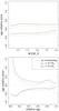 |
Fig. 10 Envelope of age estimate relative errors due to sampling from synthetic grids with different values of convective core overshooting extension lov. Ages are estimated on the standard grid without overshooting. |
As usually happens, the bias in age estimate is essentially the consequence of the bias in mass. In V14 the effect of overshooting on mass estimates was not studied since the range of mass was different, so we present the basic results here. Figure 11 shows the effect on mass estimates of a mild overshooting β = 0.2. The effect of the overshooting is evident around relative ages from 0.7 to 0.9. In this zone the morphology of the grids computed with and without overshooting is most different, since the overall contraction starts in different regions of the two grids. This causes the strong bias towards the mass underestimation visible in Fig. 11. When the overall contraction phase ends and the tracks again evolve in parallel (relative age around 0.9), the bias suddenly disappears.
Since the strongest bias occurs in the same region where the impact of weighted estimates is higher, we also show in the figure the weighted estimate envelopes for standard and mild overshooting scenarios. As discussed above, the weighting biases the mass estimates towards higher values; the effect partially counterbalances – in the relative age range from 0.7 to 0.8 – the effect of the overshooting, resulting in a final less biased estimates.
Turning again to age, the trends in the relative age error envelopes in Fig. 10 show the signature of the mass bias discussed above. We also note that around relative age 0.8, the standard envelope of the relative age errors shows inflation, which is caused by the degeneracy present in the grids during the overall contraction phase (see Sect. 3). Since several tracks accumulate and cross in this zone, the grid estimation procedure is intrinsically more difficult here. At relative ages of about 0.9, the age estimates for the overshooting scenarios show a sudden bias towards lower ages. Such an occurrence can be understood by remembering that models with convective core overshooting evolve more slowly than standard models until this phase, and faster after.
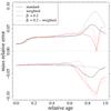 |
Fig. 11 Envelope of mass estimate relative errors for the reference case (black solid line) and for the weighted estimates (dashed black line). The red lines correspond to the overshooting scenario with β = 0.2 (red solid line) and to the same scenario when adopting weighted estimates (red dashed line). |
4.5. Element diffusion
In V14 we discussed the importance of considering the effects of the microscopic diffusion when determining stellar parameters by means of grid-based techniques, assessing the bias in mass and radius estimates when element diffusion is neglected. A similar analysis was performed here for age estimates. As in V14, we followed a slightly different approach from the previous sections. We think that it is more realistic in this case to build the artificial stars by sampling N = 50 000 objects from the standard grid of models, which takes the element diffusion into account, and to use non-standard models, which neglect elements diffusion, for the recovery.
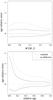 |
Fig. 12 Envelope of age-estimate relative errors obtained by including (standard) or neglecting diffusion in the reconstruction grid. At variance with previous figures, in this case the synthetic dataset is sampled from the standard grid. |
The results of the test are presented in the section “no diffusion” of Tables 1 and 2 and in Fig. 12. In this case the bias is very strong, reaching values of about 40% for stars of mass lower than 1.1 M⊙. As expected, the bias is lower for more massive objects owing to the fast evolutionary time scale with respect to the diffusion one. The bias due to the neglect of diffusion is close to the 1σ random uncertainty of the standard models, therefore the systematic bias due to this source of uncertainty could significantly affect the age estimates obtained using grids that do not take diffusion into account. Thus, it would be important to improve the treatment of diffusion in the current generation of stellar computations in order to properly follow the evolution of surface chemical abundances.
5. Comparison with other pipelines
The results presented in the previous sections were obtained by using models from a single stellar evolutionary code, and they allow a precise characterization of the impact of the various input and parameters that influence stellar evolution. However, they do not make the evaluation of systematic biases possible owing to the adoption of different codes. As already reported in the literature (see e.g. Gai et al. 2011; Mathur et al. 2012; Chaplin et al. 2014), the adoption of different grids and estimation procedures can produce age estimates with systematic variance within an order of magnitude of the statistical uncertainties due to the observational errors.
A comparison of our results with those obtained by other techniques will contribute to assessing such a systematic bias. In this section we present mass and age estimates of several objects from the observational samples studied in Mathur et al. (2012) and Chaplin et al. (2014, hereafter M12 and C14, respectively).
SCEPtER unweighted age and mass estimates for the observational sample from Mathur et al. (2012).
For the first comparison we selected twenty objects analysed in M12 by adopting RADIUS, YB, and SEEK techniques (Stello et al. 2009; Gai et al. 2011; Quirion et al. 2010). We excluded two objects from the original sample, K8760414 and K11713510, because the observed metallicity of the first one is outside our grid, and only the SEEK estimates are available for the second one. The seismic and non-seismic observational constraints adopted in the analysis are presented in Tables 2 and 3 of M12; for the solar values we adopt, as in M12, νmax, ⊙ = 3050 μHz and Δν⊙ = 135 μHz. Uncertainties of 30 μHz on νmax, ⊙ and 0.1 μHz on Δν⊙ were considered by error propagation in the uncertainty of νmax and Δν.
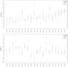 |
Fig. 13 SCEPtER age and mass estimates for the observational sample from Mathur et al. (2012), compared with those by RADIUS, YB, and SEEK. Objects were sorted by ascending SCEPtER estimated age. |
The SCEPtER mass and age estimates for the selected sample are in Table 3. Since neither YB nor RADIUS take the evolutionary time scale into account, for this comparison we adopted unweighted estimates. In Fig. 13 we compare the SCEPtER estimates with those of RADIUS, YB, and SEEK reported in M12. A general agreement amongst the estimates of the four techniques is found. For ten objects, the standard deviation of the pipelines estimates is lower than the corresponding random error, obtained by averaging the errors of the four pipelines, and only for four objects is the computed standard deviation greater than two times the random component. For nine objects (K4914923, K5184732, K5512589, K6603624, K6933899, K7680114, K7976303, K8006161, and K10963065), age estimates all agree within their errors. Regarding the mass, the same occurs for five objects (K3632418, K5512589, K6106415, K7976303, and K10963065). Thus age and mass are in overall agreement for three objects (K5512589, K7976303, and K10963065). However, this comparison is probably not fully appropriate, since the estimates of different pipelines are probably highly correlated. To illustrate this point, let us focus on a YB versus SCEPtER comparison, which adopts the same estimation scheme. The two techniques obtain their error bars by scattering the observational values by Monte Carlo perturbation within the observational uncertainties. We consider a hypothetical comparison for which the estimates of the two pipelines were performed on the same perturbed set. It can be argued that a perturbation that forces YB to overestimate the age with respect to its mean value has a similar impact on the SCEPtER estimate. This correlation should be taken into account in a comparison of the estimated values, and the usual consistency within error bars is probably misleading. The actual correlation among estimates could not be evaluated here since we do not have access to the other pipelines to quantify the effect.
A safer comparison involves only the estimates of the different pipelines, disregarding their errors. The observational sample is large enough to allow a formal statistical analysis. We are interested in possible systematic differences in mass and age estimates from the four techniques.
The dataset under examination presented, for each star, four estimates of mass and four of age. To take into account that repeated measurements were available for each object and to increase the statistical power of the test, a two-way ANOVA design was adapted to the data. Since the four pipeline estimates are performed on the same set of stars, the model allows extracting the variance due to the mean difference amongst the age and mass estimated for the stars in the sample, allowing a more powerful assessment of the differences amongst the various pipelines. The hypotheses for a parametric ANOVA were not satisfied owing to a large inhomogeneity of variances in the groups, so the analysis was conducted by adopting the Friedman test, which is the non-parametric analogue of a two-way ANOVA (Conover 1999).
No significant difference was found amongst the stellar masses estimated by the four techniques (Friedman χ2 = 5.89, df = 3, p-value = 0.12). This implies that the hypothesis of no systematic bias due to the choice of a particular pipeline in the recovered mass cannot be rejected. However, data provide an indication that SEEK tends to overestimate the stellar mass with respect to the other techniques. The median differences of the SEEK masses with respect to those estimated by SCEPtER, RADIUS, and YB are 0.04, 0.06, and 0.045 M⊙, respectively. These differences do not reach the significance level because of the low statistical power attainable with the available sample size.
Age estimations: tukey multiple comparisons of means for the four pipelines examined in the text.
In the case of age estimates, a significant difference amongst the pipelines was shown (Friedman χ2 = 16.98, df = 3, p-value = 0.0071). To assess the origin of this difference, we performed a post-hoc Tukey honest significant differences test (see e.g. Hsu 1996; Snedecor & Cochran 1989), comparing all the possible pairs of mean of age estimates between the pipelines. Since the hypotheses of ANOVA are violated, the test was performed on the rank of the data8, computed for each star (Conover 1999).
The results of the test are presented in Table 4 where we show the rank differences between groups, the median of the age differences between groups, and the p values of the tests. We found that the SCEPtER age estimates agree with all the other pipelines except YB, which gives significantly higher ages with a median difference of 0.99 Gyr (p-value = 0.0069). Regarding the other pipelines inter-comparisons, SEEK age estimates are in median 0.89 Gyr lower than those from RADIUS (p-value = 0.015) and 0.93 Gyr lower than those from YB (p-value = 0.00078).
As a second comparison we evaluated the masses and ages of 73 objects analysed in C14, for which spectroscopic constraints were available from Bruntt et al. (2012). These stars were selected from the sample of 87 stars reported in Table 2 of C14. We excluded 14 objects lying outside our estimation grid.
The mass and age estimates presented in C14 have been obtained from Bellaterra Stellar Properties Pipeline (BeSPP) coupled with a grid constructed by the GARSTEC code (Weiss & Schlattl 2008); the parameters of the grid are described in Silva Aguirre et al. (2012). The Δν of each model in this grid was determined using the calculated frequencies of each model. The error budget includes the contribution of the systematic differences due to other pipelines examined in C14. In this analysis we adopt for the solar values, as in C14, νmax, ⊙ = 3090 μHz and Δν⊙ = 135.1 μHz. Uncertainties of 30 μHz on νmax, ⊙ and 0.1 μHz on Δν⊙ were considered by error propagation in the uncertainty of νmax and Δν. In this comparison we adopted weighted estimates, since this effect is accounted for in the BeSPP pipeline.
Table 5 presents the SCEPtER estimates of age and mass. In Fig. 14 these estimates are compared with the one given in C14. The estimates are consistent within their errors with the exceptions of K3424541, K8367710, and K11026764. The same caveat as was discussed in the previous comparison about neglecting the estimate correlations applies here.
The formal analysis of the differences in the estimates of the two pipelines was then performed by the paired t-test. A significant difference (p-value < 2 × 10-16) was found in the mass estimates; BeSPP estimates of stellar masses were 0.052 M⊙ (95% confidence interval [0.043; 0.061] M⊙) higher than those of SCEPtER. Besides the statistical significance, this bias is also relevant from the stellar evolution point of view, since it is the same as the average error due to the observational uncertainty, which is 0.054 M⊙ for SCEPtER and 0.068 M⊙ for BeSPP. The difference amongst age estimates did not reach the significance (p-value = 0.37), and BeSPP age estimates are 0.06 Gyr (95% confidence interval [−0.20; 0.08] Gyr) higher than those of SCEPtER. This bias is also small with respect to the random errors due to observational uncertainty, which are about 0.88 Gyr for SCEPtER and 1.00 Gyr for BeSPP, and it can be safely disregarded from the stellar evolutionary point of view. These results suggest that the evolutionary time scale is different in the two stellar grids, since stars of different masses turn out to have a similar age.
SCEPtER age and mass estimates for the observational sample from Chaplin et al. (2014).
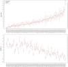 |
Fig. 14 SCEPtER weighted age and mass estimates for the observational sample from Chaplin et al. (2014), compared with that by BeSPP. |
The large sample size allowed us a further test of the differences between the estimates from SCEPtER and BeSPP sub-setting the objects into homogeneous groups. In fact the small difference between the two pipelines may occur either because they provide consistent estimates on the whole set of stars or because a compensation between opposite differences in subsets of stars occurs.
The first step in the analysis was to identify a natural partition of the dataset, based only on the four observational quantities (Teff, [Fe/H] Δν, νmax) adopted in the grids. We performed this step by a well established statistical procedure, which is an agglomerative hierarchical cluster analysis (see e.g. Kaufman & Rousseeuw 1990; Härdle & Simar 2012) on the 73 stellar objects. Details on the adopted technique are provided in Appendix B. Following the analysis, data were split into two groups, the first containing more massive (interquartile range [1.20; 1.36] M⊙) and less metallic (mean [Fe/H] = −0.06 dex) objects with respect to the second one (mean SCEPtER estimated mass 1.08 M⊙ with interquartile range [1.00; 1.14] M⊙, mean [Fe/H] = 0.03 dex).
The subsequent statistical analysis of the two groups (see e.g. Appendix B for details) revealed that the estimates of the two pipelines have an unequal difference in the two groups. While the median estimates of SCEPtER was 0.19 Gyr higher for less massive objects, for massive stars it was 0.61 Gyr lower. The difference could be due to the fact that the grid used by BeSPP includes a mild overshooting and neglects the microscopic diffusion for masses higher than 1.4 M⊙. As seen in Sect. 4, both the differences lead to higher age estimates for massive models.
6. Conclusions
We performed a theoretical investigation aimed to quantify the effect of the current uncertainties in stellar models on the estimates of star ages obtained by means of grid-based techniques, adopting asteroseismic constraints. We analysed the uncertainties arising from several inputs of stellar model computations: input physics, chemical composition, and the efficiency of microscopic processes.
To this purpose, we used our grid-based pipeline SCEPtER (Valle et al. 2014). As observational constraints, we adopted the stellar effective temperature, its metallicity [Fe/H], the large frequency spacing Δν, and the frequency of maximum oscillation power νmax of the star. The grid of stellar models, computed for the evolutionary phases from ZAMS to the central hydrogen depletion, has been extended to cover the mass range [0.8; 1.6] M⊙.
We compared the statistical errors arising from the uncertainties in observational quantities with the systematic biases due to the uncertainties in initial helium content, in the mixing-length parameter value, in the convective core overshooting, and in the microscopic diffusion. We also explored the impact of the uncertainty on radiative opacities, which is the most relevant input physics with respect to uncertainty propagation (see Valle et al. 2013a,b, for a detailed discussion). This is the first time that a comprehensive detailed theoretical analysis has been performed.
We found that the statistical error component in age estimates strongly depends on the relative age of the star. The 1σ relative error envelope, averaged over all the stellar masses, is larger than 120% and highly asymmetric for stars near the ZAMS, while it is about 20−30% and more symmetric at later ages. The dependence on the stellar mass is less important and is influenced by edge effects. The 1σ envelope, averaged over all the evolutionary stages, typically extends from +42% to +30% (upper boundary) and from −35% to −20% (lower boundary) for masses from 0.90 M⊙ to 1.40 M⊙.
We studied the impact of varying the initial helium abundance by changing of ±1 the helium-to-metal enrichment ratio ΔY/ΔZ. The systematic bias is small in the explored range, except for stars near the ZAMS. For relative ages older than 0.2 the bias drops under a value of about 10%. Overall, the helium bias is about one-third of the width of the envelope due to the random observational uncertainties.
The impact of the uncertainty on radiative opacities was studied here for the first time. We found that the current uncertainty in radiative opacities – i.e. ±5% – does not influence the age estimates from grid techniques.
The efficiency of the super-adiabatic convection represents one of the weakest points in theoretical stellar evolution. We studied the impact of varying the mixing-length parameter by computing several synthetic grids with αml from 1.50 to 1.98, with our solar calibrated value (i.e. αml = 1.74) adopted as a reference for the recovery standard grid. The impact of this source of bias, for models of mass lower than 1.2 M⊙, was found to be strong with values of about −20% for αml = 1.98 and of about 30% for αml = 1.50. The bias is lower for higher mass models owing to the decreasing thickness of the convective envelope. Therefore the mixing-length value adopted in the reconstruction can bias the estimates in a significant way.
The lack of a self-consistent treatment of convection in stars prevents a firm and robust prediction of convective core extension. We quantified the resulting bias on grid-based age estimates by computing two additional sets of stellar models taking convective core overshooting with β = 0.2 and 0.4 into account. The bias due to the mild-overshooting scenario is at most about −7% for models of 1.5 M⊙, while for β = 0.4 it reaches −13%. Since these values are low compared to the standard envelope due to random errors on the observables adopted in the reconstruction, the convective core overshooting can be considered as a minor source of bias.
Some grid-based techniques, such as RADIUS (Stello et al. 2009) and SEEK, which both adopt a grid of models computed with the Aarhus STellar Evolution Code (Christensen-Dalsgaard 2008), do not implement diffusion. We evaluated the bias caused by this neglect and found that it is very strong, reaching values of about 40% for models of mass lower than 1.1 M⊙. The bias is less for higher mass models owing to the fast evolutionary time scale compared to the diffusion one. The diffusion-induced bias is close to or greater than the uncertainty arising from random errors in the observables.
We compared the results obtained by the SCEPtER technique to those found by adopting other grid-based techniques reported in the literature: RADIUS (Stello et al. 2009), YB (Gai et al. 2011), SEEK (Christensen-Dalsgaard 2008), and BeSPP (Serenelli et al. 2013). We selected a homogeneous subset of several targets from the Kepler catalogue, already studied in Mathur et al. (2012) and Chaplin et al. (2014). No significant difference was found amongst the stellar mass estimated by SCEPtER, RADIUS, YB, and SEEK; while age estimates of these four pipelines significantly differ. Age estimates by YB are significantly higher than SCEPtER ones, with a median difference of 0.99 Gyr; SEEK age estimates are on average 0.89 Gyr lower than those by RADIUS and 0.93 Gyr lower than those by YB. The comparison of age estimates by SCEPtER and BeSPP showed overall agreement, whereas a significant difference was found in the mass estimates, since BeSPP estimation of stellar masses are 0.052 M⊙ higher than those of SCEPtER. BeSPP age estimates are only 0.07 Gyr higher; however, we verified that by splitting objects into two subgroups, the age of massive objects is generally overestimated by BeSPP.
Online material
Appendix A: Mass and radius estimates
The statistical error and the systematic bias due to the uncertainty sources considered in this paper were addressed in V14, but only for a maximum stellar mass of 1.1 M⊙. In this Appendix we report some results about mass and radius estimate obtained in the extended range considered in this paper.
The results presented in V14 are still valid in this broader range. Since the relative error on mass and radius is nearly independent of the relative age and on the mass – neglecting the edge effect – we adopt here the same technique as in Valle et al. (2014) and report the median bias of mass and radius relative error and the sample standard deviations for the considered uncertainty source.
Figure A.1 shows, for the standard case of stars sampled and reconstructed on the standard grid, the trend of mass and radius relative error versus the true mass of the star, its relative age, and its metallicity. It is apparent that the same discussion of V14 retains its validity. In particular, the strong edge effect is evident in the mass panel, as are the inflation of variance at high relative age noted and discussed in the previous paper of the series.
The analysis of the impact of the considered uncertainties is summarized in Table A.1. The biases and the standard errors are very similar to the ones reported in V14. Therefore the results presented in the previous paper also remain valid for more massive objects.
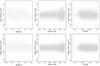 |
Fig. A.1 Top row: relative error on mass estimate with respect to the true mass of the star, to its relative age and its metallicity [Fe/H]. Bottom row: same as the top row but for radius relative errors. |
Summary of mass and radius relative errors.
Appendix B: Differences between SCEPtER and BeSPP age estimates
The first step in the analysis was to identify a natural partition of the dataset, based only on the four observational quantities (Teff, [Fe/H] Δν, νmax) adopted in the grids. The technique starts with each observation forming a cluster by itself. Clusters are subsequently merged until only one cluster containing all the observations remains. At each step the two nearest clusters are combined to form one larger cluster. The analysis was performed by adopting the Ward’s clustering method to define the cluster similarity (Kaufman & Rousseeuw 1990). The computations were performed using R 3.1.0 (R Development Core Team 2014) by mean of the functions in the package cluster (Maechler et al. 2014).
More technically, let X be the matrix of the p observed quantities for the n objects under consideration. Before the analysis, the columns of X are standardized; that is, all the columns are scaled to zero mean and unit variance. Let xij be the element of the ith row and jth column of X. Let D be the n × n dissimilarity matrix for the n object, which is the matrix whose elements dij are the Euclidean distances between rows i and j of X.
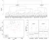 |
Fig. B.1 Top row: hierarchical cluster analysis of the observational sample adopted in SCEPtER and BeSPP comparison. The dashed line marks the sub-setting into two groups suggested by the silhouette plot analysis (see text). Bottom row, left: separation of the two group in the plane (Teff − Δν). Bottom row, right: boxplot of age estimates of the two pipelines in the two groups. |
At each step, the clustering algorithm merges the two nearest clusters. The first step is trivial since each object forms a cluster containing exactly one object, and therefore the two nearest objects are merged. For the second step, a definition of distance amongst clusters containing more than one object is needed. Let A and B be two objects joined in a single group A + B; the distance between this group and a group C is ![\appendix \setcounter{section}{2} \begin{eqnarray} d(C, A+B)& = &\delta_1 d(C,A) + \delta_2 d(C,B) + \delta_3 d(A,B)\notag \\ \label{eq:distance} &&+ \delta_4[d(C,A) - d(C,B)]. \end{eqnarray}](/articles/aa/full_html/2015/03/aa24686-14/aa24686-14-eq261.png) (B.1)Different choices of the weights δ1,...,4 provide different clustering algorithms. We adopt the Ward’s weighting, which minimizes the heterogeneity within clusters (see e.g. Härdle & Simar 2012)
(B.1)Different choices of the weights δ1,...,4 provide different clustering algorithms. We adopt the Ward’s weighting, which minimizes the heterogeneity within clusters (see e.g. Härdle & Simar 2012) ![\appendix \setcounter{section}{2} \begin{eqnarray} \delta_1 & = & \frac{n_C+n_A}{n_A+n_B+n_C}\nonumber\\[0.5mm] \delta_2 & = & \frac{n_C+n_B}{n_A+n_B+n_C}\nonumber\\[0.5mm] \delta_3 & = & -\frac{n_C}{n_A+n_B+n_C}\nonumber\\ \delta_4 & = & 0. \end{eqnarray}](/articles/aa/full_html/2015/03/aa24686-14/aa24686-14-eq263.png) (B.2)The clustering is repeated until all the observations are in the same cluster.
(B.2)The clustering is repeated until all the observations are in the same cluster.
The result of the analysis is shown in the dendrogram in the top row of Fig. B.1. The height of the nodes is the distance, as defined in Eq. (B.1), at which the corresponding clusters merge. The lower a node, the more similar the merged clusters. Cutting the dendrogram at different heights (as done by the dashed line in the figure) produces a different number of sub-groups. The optimal number of groups suggested by the clustering was determined according to silhouette plot analysis (Rousseeuw 1987; Kaufman & Rousseeuw 1990) which, for each object, provides a value (silhouette) which shows how well the object lies within its cluster. The clustering providing the largest average silhouette is chosen as the best one. As a result, the two groups split, as shown in the figure by the dashed line that turned out to be the optimal one.
The algorithmic approach to constructing a silhouette is the following. For each object i, let a(i) be the average distance among i and all other object inside the same cluster. Then, for all the other clusters C, let d(i,C) be the average distance of i and all the elements of C. Let b(i) be the minimum value of d(i,C) over all the clusters C. The silhouette s(i) is then  (B.3)When a cluster contains a single object, then by definition s(i) = 0. A high value of s(i) implies that an observation lies well inside its cluster, while a value near 0 indicates that the observation lies equally well inside its cluster or in the nearest one. A negative silhouette suggests that the object is possibly in the wrong group. By averaging the values of s(i) over all the objects, one obtains the average silhouette that is used for diagnostic purposes. In our case the average silhouette for a two-group clustering is 0.35, while for a three groups it drops to 0.29. Therefore a two-group split is preferred.
Group 1 contains more massive (mean SCEPtER estimated mass 1.27 M⊙, interquartile range [1.20; 1.36] M⊙) and less metallic (mean [Fe/H] = −0.06 dex) objects with respect to the second one (mean SCEPtER estimated mass 1.08 M⊙ with interquartile range [1.00; 1.14] M⊙, mean [Fe/H] = 0.03 dex). The separation of the two groups in the plane (Teff − Δν) is shown in the bottom row, left-hand panel of Fig. B.1. The two identified groups of stars are mainly split by their Δν values.
Having defined a grouping for the stars, we repeated the statistical analysis of the differences among pipelines, but also taking the group split into account. This was done by adapting a mixed-design model to data (see e.g. Snedecor & Cochran 1989; Faraway 2004). This experimental design takes the hierarchy in the data into account and contains between-object variables (the group variable) and within-object variables, allowing for a different level of variability to be accounted for between and within objects. In other words, the model includes a level of variation in addition to the per-observation noise term that it is accounted for in common statistical models such as linear regression models.
The adoption of a nesting variable (the individual stars) allows considering that a couple of estimates exist for each star. The other variables in the models are the pipeline adopted for estimations (categorical variable with level BeSPP and SCEPtER), the subgroup of star (categorical at two levels), and their interaction, which is the variable of interest in the analysis. A significant interaction means that the two pipeline estimates vary differently in the two groups. The model was analysed adapting a mixed-design ANOVA model (also known as repeated measurements ANOVA or split-plot design) to data. The result of the analysis is presented in Table B.1. The conclusion is that the age estimates by the two pipelines vary in significantly different ways (p-value = 2.4 × 10⁻⁵) from one group to the next. As shown in the right-hand panel in the bottom row of Fig. B.1, the estimates of the two pipelines are very close for less massive stars, while those of BeSPP are significantly higher for massive objects. The differences in median SCEPtER versus BeSPP age estimates for a lighter star is 0.19 Gyr, while for massive models it is −0.61 Gyr. It is relevant to note that the mass estimates do not suffer from a differential effect like the one present for ages. The same analysis as detailed above, which was repeated with mass as dependent variable, does not reveal a significant interaction (p-value = 0.40).
The conclusion of the analysis is therefore that the two pipelines differ in the evolutionary time scale (the age of less massive stars is similar although their mass are estimated different), and the difference in evolutionary time scale changes from massive to light stars.
ANOVA table for the analysis of the differences between SCEPtER and BeSPP.
An R library providing the estimation code and grid is available at CRAN: http://CRAN.R-project.org/package=SCEPtER
A boxplot is a convenient way to summarize the variability of the data; the black thick lines show the median of the data set, while the box marks the interquartile range; i.e., it extends form the 25th to the 75th percentile of data. The whiskers extend from the box until the extreme data, but they can only extend to a maximum of 1.5 times the width of the box.
Acknowledgments
We thank our anonymous referee for many comments and suggestions that largely helped clarify and improve the paper. This work has been supported by PRIN-MIUR 2010−2011 (Chemical and dynamical evolution of the Milky Way and Local Group galaxies, PI F. Matteucci), PRIN-INAF 2011 (Tracing the formation and evolution of the Galactic Halo with VST, PI M. Marconi), and PRIN-INAF 2012 (The M4 Core Project with Hubble Space Telescope, PI L. Bedin).
References
- Appourchaux, T., Michel, E., Auvergne, M., et al. 2008, A&A, 488, 705 [NASA ADS] [CrossRef] [EDP Sciences] [Google Scholar]
- Asplund, M., Grevesse, N., Sauval, A. J., & Scott, P. 2009, ARA&A, 47, 481 [NASA ADS] [CrossRef] [Google Scholar]
- Baglin, A., Auvergne, M., Barge, P., et al. 2009, in IAU Symp. 253, eds. F. Pont, D. Sasselov, & M. J. Holman, 71 [Google Scholar]
- Basu, S., Chaplin, W. J., & Elsworth, Y. 2010, ApJ, 710, 1596 [NASA ADS] [CrossRef] [Google Scholar]
- Basu, S., Verner, G. A., Chaplin, W. J., & Elsworth, Y. 2012, ApJ, 746, 76 [NASA ADS] [CrossRef] [Google Scholar]
- Bonaca, A., Tanner, J. D., Basu, S., et al. 2012, ApJ, 755, L12 [NASA ADS] [CrossRef] [Google Scholar]
- Borucki, W. J., Koch, D., Basri, G., et al. 2010, Science, 327, 977 [NASA ADS] [CrossRef] [PubMed] [Google Scholar]
- Bruntt, H., Basu, S., Smalley, B., et al. 2012, MNRAS, 423, 122 [NASA ADS] [CrossRef] [Google Scholar]
- Casagrande, L., Schönrich, R., Asplund, M., et al. 2011, A&A, 530, A138 [NASA ADS] [CrossRef] [EDP Sciences] [Google Scholar]
- Chaboyer, B., Fenton, W. H., Nelan, J. E., Patnaude, D. J., & Simon, F. E. 2001, ApJ, 562, 521 [NASA ADS] [CrossRef] [Google Scholar]
- Chaplin, W. J., Basu, S., Huber, D., et al. 2014, ApJS, 210, 1 [NASA ADS] [CrossRef] [Google Scholar]
- Christensen-Dalsgaard, J. 2008, Ap&SS, 316, 13 [NASA ADS] [CrossRef] [Google Scholar]
- Clausen, J. V., Bruntt, H., Claret, A., et al. 2009, A&A, 502, 253 [NASA ADS] [CrossRef] [EDP Sciences] [Google Scholar]
- Conover, W. 1999, Practical nonparametric statistics, Wiley series in probability and statistics: Applied probability and statistics (Wiley) [Google Scholar]
- Cyburt, R. H., Fields, B. D., & Olive, K. A. 2004, Phys. Rev. D, 69, 123519 [NASA ADS] [CrossRef] [Google Scholar]
- Degl’Innocenti, S., Pra da Moroni, P. G., Marconi, M., & Ruoppo, A. 2008, Ap&SS, 316, 25 [NASA ADS] [CrossRef] [Google Scholar]
- Deheuvels, S., & Michel, E. 2011, A&A, 535, A91 [NASA ADS] [CrossRef] [EDP Sciences] [Google Scholar]
- Dell’Omodarme, M., & Valle, G. 2013, The R Journal, 5, 108 [Google Scholar]
- Dell’Omodarme, M., Valle, G., Degl’Innocenti, S., & Pra da Moroni, P. G. 2012, A&A, 540, A26 [NASA ADS] [CrossRef] [EDP Sciences] [Google Scholar]
- Epstein, C. R., & Pinsonneault, M. H. 2014, ApJ, 780, 159 [NASA ADS] [CrossRef] [Google Scholar]
- Faraway, J. J. 2004, Linear Models with R (Chapman & Hall/CRC) [Google Scholar]
- Gai, N., Basu, S., Chaplin, W. J., & Elsworth, Y. 2011, ApJ, 730, 63 [NASA ADS] [CrossRef] [Google Scholar]
- Gennaro, M., Prada Moroni, P. G., & Degl’Innocenti, S. 2010, A&A, 518, A13 [NASA ADS] [CrossRef] [EDP Sciences] [Google Scholar]
- Gilliland, R. L., Brown, T. M., Christensen-Dalsgaard, J., et al. 2010, PASP, 122, 131 [NASA ADS] [CrossRef] [Google Scholar]
- Härdle, W. K., & Simar, L. 2012, Applied Multivariate Statistical Analysis (Springer) [Google Scholar]
- Hsu, J. 1996, Multiple Comparisons: Theory and Methods (Taylor & Francis) [Google Scholar]
- Huber, D., Chaplin, W. J., Christensen-Dalsgaard, J., et al. 2013, ApJ, 767, 127 [NASA ADS] [CrossRef] [Google Scholar]
- Jimenez, R., Flynn, C., MacDonald, J., & Gibson, B. K. 2003, Science, 299, 1552 [NASA ADS] [CrossRef] [PubMed] [Google Scholar]
- Jørgensen, B. R., & Lindegren, L. 2005, A&A, 436, 127 [NASA ADS] [CrossRef] [EDP Sciences] [Google Scholar]
- Kaufman, L., & Rousseeuw, P. J. 1990, Finding groups in data: an introduction to cluster analysis (New York: John Wiley and Sons) [Google Scholar]
- Kjeldsen, H., & Bedding, T. R. 1995, A&A, 293, 87 [NASA ADS] [Google Scholar]
- Lebreton, Y. 2013, EAS Pub. Ser., 63, 123 [Google Scholar]
- Lebreton, Y., & Montalbán, J. 2009, in IAU Symp. 258, eds. E. E. Mamajek, D. R. Soderblom, & R. F. G. Wyse, 419 [Google Scholar]
- Maechler, M., Rousseeuw, P., Struyf, A., Hubert, M., & Hornik, K. 2014, cluster: Cluster Analysis Basics and Extensions, r package version 1.15.2 – For new features, see the Changelog file (in the package source) [Google Scholar]
- Magic, Z., Weiss, A., & Asplund, M. 2015, A&A, 573, A89 [NASA ADS] [CrossRef] [EDP Sciences] [Google Scholar]
- Mathur, S., Metcalfe, T. S., Woitaszek, M., et al. 2012, ApJ, 749, 152 [NASA ADS] [CrossRef] [Google Scholar]
- Metcalfe, T. S., Creevey, O. L., Dogan, G., et al. 2014, ApJS, 214, 27 [NASA ADS] [CrossRef] [Google Scholar]
- Michel, E., Baglin, A., Auvergne, M., et al. 2008, Science, 322, 558 [NASA ADS] [CrossRef] [PubMed] [Google Scholar]
- Pagel, B. E. J., & Portinari, L. 1998, MNRAS, 298, 747 [NASA ADS] [CrossRef] [Google Scholar]
- Peimbert, M., Luridiana, V., & Peimbert, A. 2007a, ApJ, 666, 636 [NASA ADS] [CrossRef] [Google Scholar]
- Peimbert, M., Luridiana, V., Peimbert, A., & Carigi, L. 2007b, in From Stars to Galaxies: Building the Pieces to Build Up the Universe, eds. A. Vallenari, R. Tantalo, L. Portinari, & A. Moretti, ASP Conf. Ser., 374, 81 [Google Scholar]
- Pont, F., & Eyer, L. 2004, MNRAS, 351, 487 [NASA ADS] [CrossRef] [Google Scholar]
- Quirion, P.-O., Christensen-Dalsgaard, J., & Arentoft, T. 2010, ApJ, 725, 2176 [NASA ADS] [CrossRef] [Google Scholar]
- R Development Core Team. 2014, R: A Language and Environment for Statistical Computing, R Foundation for Statistical Computing, Vienna, Austria [Google Scholar]
- Rousseeuw, P. J. 1987, J. Comput. Appl. Math., 20, 53 [Google Scholar]
- Scott, D. W. 1992, Multivariate Density Estimation. Theory, Practice and Visualization (Wiley) [Google Scholar]
- Serenelli, A. M., Bergemann, M., Ruchti, G., & Casagrande, L. 2013, MNRAS, 429, 3645 [NASA ADS] [CrossRef] [Google Scholar]
- SilvaAguirre, V., Casagrande, L., Basu, S., et al. 2012, ApJ, 757, 99 [NASA ADS] [CrossRef] [Google Scholar]
- Silva Aguirre, V., Basu, S., Brandão, I. M., et al. 2013, ApJ, 769, 141 [NASA ADS] [CrossRef] [Google Scholar]
- Snedecor, G., & Cochran, W. 1989, Statistical methods, Statistical Methods No. v. 276 (Iowa State University Press) [Google Scholar]
- Soderblom, D. R. 2010, ARA&A, 48, 581 [NASA ADS] [CrossRef] [Google Scholar]
- Steigman, G. 2006, Int. J. Mod. Phys. E, 15, 1 [Google Scholar]
- Stello, D., Chaplin, W. J., Bruntt, H., et al. 2009, ApJ, 700, 1589 [NASA ADS] [CrossRef] [Google Scholar]
- Tanner, J. D., Basu, S., & Demarque, P. 2014, ApJ, 785, L13 [NASA ADS] [CrossRef] [Google Scholar]
- Thoul, A. A., Bahcall, J. N., & Loeb, A. 1994, ApJ, 421, 828 [NASA ADS] [CrossRef] [Google Scholar]
- Trampedach, R., & Stein, R. F. 2011, ApJ, 731, 78 [NASA ADS] [CrossRef] [Google Scholar]
- Ulrich, R. K. 1986, ApJ, 306, L37 [NASA ADS] [CrossRef] [Google Scholar]
- Valle, G., Marconi, M., Degl’Innocenti, S., & Pra da Moroni, P. G. 2009, A&A, 507, 1541 [NASA ADS] [CrossRef] [EDP Sciences] [Google Scholar]
- Valle, G., Dell’Omodarme, M., Prada Moroni, P. G., & Degl’Innocenti, S. 2013a, A&A, 549, A50 [NASA ADS] [CrossRef] [EDP Sciences] [Google Scholar]
- Valle, G., Dell’Omodarme, M., Prada Moroni, P. G., & Degl’Innocenti, S. 2013b, A&A, 554, A68 [NASA ADS] [CrossRef] [EDP Sciences] [Google Scholar]
- Valle, G., Dell’Omodarme, M., Prada Moroni, P. G., & Degl’Innocenti, S. 2014, A&A, 561, A125 (V14) [NASA ADS] [CrossRef] [EDP Sciences] [Google Scholar]
- Venables, W., & Ripley, B. 2002, Modern applied statistics with S, Statistics and computing (Springer) [Google Scholar]
- Weiss, A., & Schlattl, H. 2008, Ap&SS, 316, 99 [NASA ADS] [CrossRef] [Google Scholar]
- Yıldız, M. 2007, MNRAS, 374, 1264 [NASA ADS] [CrossRef] [Google Scholar]
All Tables
SCEPtER median (q50) and 1σ envelope boundaries (q16 and q84) for age relative error as a function of the mass of the star.
SCEPtER median (q50) and 1σ envelope boundaries (q16 and q84) for age relative error as a function of the relative age of the star.
SCEPtER unweighted age and mass estimates for the observational sample from Mathur et al. (2012).
Age estimations: tukey multiple comparisons of means for the four pipelines examined in the text.
SCEPtER age and mass estimates for the observational sample from Chaplin et al. (2014).
All Figures
|
Fig. 1 Age estimate relative errors as a function of the true mass (left panel), relative age (central panel), and metallicity [Fe/H] (right panel) of the star. The blue long dashed lines mark the error medians. The red solid line is the 1σ error envelope, while the red dashed one marks the position of the 2σ envelope (see text). A positive relative error indicates that the reconstructed age of the star is overestimated with respect to the true one. |
| In the text | |
|
Fig. 2 Left: lower boundary of the 2D envelope of age estimate relative errors as a function of mass and relative age of the star. Right: same as in the left panel, but for the upper envelope boundary. |
| In the text | |
|
Fig. 3 Envelope of age-estimate relative errors as a function of mass and relative age of the star for different assumptions on the observational errors. The solid line corresponds to the standard case; the dashed one to σ(Teff) = 50 K; the dotted one to σ( [ Fe/H ] ) = 0.05 dex; the dot-dashed one to σ(Δν) = 1%, σ(νmax) = 2.5%. |
| In the text | |
|
Fig. 4 Correlation between age and mass relative errors. The black circles correspond to models with relative age in the range [0.0; 0.2], the red triangles to relative ages in the range [0.2; 0.4], and the green crosses to relative ages in the range [0.4; 1.0]. |
| In the text | |
|
Fig. 5 Same as in Fig. 3, but for the comparison of standard and weighted estimates (see text for details). |
| In the text | |
|
Fig. 6 Envelope of the mass relative error for stars sampled and reconstructed on the standard grid (black solid line), and for the same sample reconstructed on the weighted grid (red dashed line). |
| In the text | |
|
Fig. 7 Left column: envelopes of age estimate relative errors due to sampling from synthetic grids with different values of ΔY/ΔZ. Ages are estimated on the standard grid with ΔY/ΔZ = 2. Middle column: same as the left column, but for sampling from synthetic grids with different values of the mixing-length parameter αml. Ages are estimated on the standard grid with αml = 1.74. Right column: same as the left column, but for sampling from synthetic grids with different values of radiative opacity kr. Ages are estimated on the standard grid. |
| In the text | |
|
Fig. 8 Dependence on the surface metallicity [Fe/H] of the envelopes of age estimate relative errors. The sampling occurs from synthetic grids with different values of ΔY/ΔZ, while ages are estimated on the standard grid with ΔY/ΔZ = 2. |
| In the text | |
|
Fig. 9 Left: boxplots of the difference in effective temperature between standard models and models with varied input or parameters. The differences have been computed for models in the same evolutionary phase. A positive value implies that the standard grid provides an higher effective temperature. Right: same as the left panel, but for age. |
| In the text | |
|
Fig. 10 Envelope of age estimate relative errors due to sampling from synthetic grids with different values of convective core overshooting extension lov. Ages are estimated on the standard grid without overshooting. |
| In the text | |
|
Fig. 11 Envelope of mass estimate relative errors for the reference case (black solid line) and for the weighted estimates (dashed black line). The red lines correspond to the overshooting scenario with β = 0.2 (red solid line) and to the same scenario when adopting weighted estimates (red dashed line). |
| In the text | |
|
Fig. 12 Envelope of age-estimate relative errors obtained by including (standard) or neglecting diffusion in the reconstruction grid. At variance with previous figures, in this case the synthetic dataset is sampled from the standard grid. |
| In the text | |
|
Fig. 13 SCEPtER age and mass estimates for the observational sample from Mathur et al. (2012), compared with those by RADIUS, YB, and SEEK. Objects were sorted by ascending SCEPtER estimated age. |
| In the text | |
|
Fig. 14 SCEPtER weighted age and mass estimates for the observational sample from Chaplin et al. (2014), compared with that by BeSPP. |
| In the text | |
|
Fig. A.1 Top row: relative error on mass estimate with respect to the true mass of the star, to its relative age and its metallicity [Fe/H]. Bottom row: same as the top row but for radius relative errors. |
| In the text | |
|
Fig. B.1 Top row: hierarchical cluster analysis of the observational sample adopted in SCEPtER and BeSPP comparison. The dashed line marks the sub-setting into two groups suggested by the silhouette plot analysis (see text). Bottom row, left: separation of the two group in the plane (Teff − Δν). Bottom row, right: boxplot of age estimates of the two pipelines in the two groups. |
| In the text | |
Current usage metrics show cumulative count of Article Views (full-text article views including HTML views, PDF and ePub downloads, according to the available data) and Abstracts Views on Vision4Press platform.
Data correspond to usage on the plateform after 2015. The current usage metrics is available 48-96 hours after online publication and is updated daily on week days.
Initial download of the metrics may take a while.