| Issue |
A&A
Volume 575, March 2015
|
|
|---|---|---|
| Article Number | A12 | |
| Number of page(s) | 20 | |
| Section | Stellar structure and evolution | |
| DOI | https://doi.org/10.1051/0004-6361/201424686 | |
| Published online | 11 February 2015 | |
Online material
Appendix A: Mass and radius estimates
The statistical error and the systematic bias due to the uncertainty sources considered in this paper were addressed in V14, but only for a maximum stellar mass of 1.1 M⊙. In this Appendix we report some results about mass and radius estimate obtained in the extended range considered in this paper.
The results presented in V14 are still valid in this broader range. Since the relative error on mass and radius is nearly independent of the relative age and on the mass – neglecting the edge effect – we adopt here the same technique as in Valle et al. (2014) and report the median bias of mass and radius relative error and the sample standard deviations for the considered uncertainty source.
Figure A.1 shows, for the standard case of stars sampled and reconstructed on the standard grid, the trend of mass and radius relative error versus the true mass of the star, its relative age, and its metallicity. It is apparent that the same discussion of V14 retains its validity. In particular, the strong edge effect is evident in the mass panel, as are the inflation of variance at high relative age noted and discussed in the previous paper of the series.
The analysis of the impact of the considered uncertainties is summarized in Table A.1. The biases and the standard errors are very similar to the ones reported in V14. Therefore the results presented in the previous paper also remain valid for more massive objects.
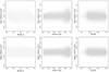 |
Fig. A.1
Top row: relative error on mass estimate with respect to the true mass of the star, to its relative age and its metallicity [Fe/H]. Bottom row: same as the top row but for radius relative errors. |
| Open with DEXTER | |
Summary of mass and radius relative errors.
Appendix B: Differences between SCEPtER and BeSPP age estimates
The first step in the analysis was to identify a natural partition of the dataset, based only on the four observational quantities (Teff, [Fe/H] Δν, νmax) adopted in the grids. The technique starts with each observation forming a cluster by itself. Clusters are subsequently merged until only one cluster containing all the observations remains. At each step the two nearest clusters are combined to form one larger cluster. The analysis was performed by adopting the Ward’s clustering method to define the cluster similarity (Kaufman & Rousseeuw 1990). The computations were performed using R 3.1.0 (R Development Core Team 2014) by mean of the functions in the package cluster (Maechler et al. 2014).
More technically, let X be the matrix of the p observed quantities for the n objects under consideration. Before the analysis, the columns of X are standardized; that is, all the columns are scaled to zero mean and unit variance. Let xij be the element of the ith row and jth column of X. Let D be the n × n dissimilarity matrix for the n object, which is the matrix whose elements dij are the Euclidean distances between rows i and j of X.
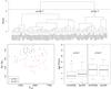 |
Fig. B.1
Top row: hierarchical cluster analysis of the observational sample adopted in SCEPtER and BeSPP comparison. The dashed line marks the sub-setting into two groups suggested by the silhouette plot analysis (see text). Bottom row, left: separation of the two group in the plane (Teff − Δν). Bottom row, right: boxplot of age estimates of the two pipelines in the two groups. |
| Open with DEXTER | |
At each step, the clustering algorithm merges the two nearest clusters. The first step is trivial since each object forms a cluster containing exactly one object, and therefore the two nearest objects are merged. For the second step, a definition of distance amongst clusters containing more than one object is needed. Let A and B be two objects joined in a single group A + B; the distance between this group and a group C is  (B.1)Different choices of the weights δ1,...,4 provide different clustering algorithms. We adopt the Ward’s weighting, which minimizes the heterogeneity within clusters (see e.g. Härdle & Simar 2012)
 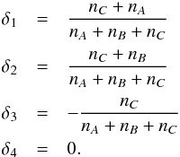 (B.2)The clustering is repeated until all the observations are in the same cluster.
The result of the analysis is shown in the dendrogram in the top row of Fig. B.1. The height of the nodes is the distance, as defined in Eq. (B.1), at which the corresponding clusters merge. The lower a node, the more similar the merged clusters. Cutting the dendrogram at different heights (as done by the dashed line in the figure) produces a different number of sub-groups. The optimal number of groups suggested by the clustering was determined according to silhouette plot analysis (Rousseeuw 1987; Kaufman & Rousseeuw 1990) which, for each object, provides a value (silhouette) which shows how well the object lies within its cluster. The clustering providing the largest average silhouette is chosen as the best one. As a result, the two groups split, as shown in the figure by the dashed line that turned out to be the optimal one.
The algorithmic approach to constructing a silhouette is the following. For each object i, let a(i) be the average distance among i and all other object inside the same cluster. Then, for all the other clusters C, let d(i,C) be the average distance of i and all the elements of C. Let b(i) be the minimum value of d(i,C) over all the clusters C. The silhouette s(i) is then 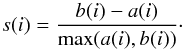 (B.3)When a cluster contains a single object, then by definition s(i) = 0. A high value of s(i) implies that an observation lies well inside its cluster, while a value near 0 indicates that the observation lies equally well inside its cluster or in the nearest one. A negative silhouette suggests that the object is possibly in the wrong group. By averaging the values of s(i) over all the objects, one obtains the average silhouette that is used for diagnostic purposes. In our case the average silhouette for a two-group clustering is 0.35, while for a three groups it drops to 0.29. Therefore a two-group split is preferred.
Group 1 contains more massive (mean SCEPtER estimated mass 1.27 M⊙, interquartile range [1.20; 1.36] M⊙) and less metallic (mean [Fe/H] = −0.06 dex) objects with respect to the second one (mean SCEPtER estimated mass 1.08 M⊙ with interquartile range [1.00; 1.14] M⊙, mean [Fe/H] = 0.03 dex). The separation of the two groups in the plane (Teff − Δν) is shown in the bottom row, left-hand panel of Fig. B.1. The two identified groups of stars are mainly split by their Δν values.
Having defined a grouping for the stars, we repeated the statistical analysis of the differences among pipelines, but also taking the group split into account. This was done by adapting a mixed-design model to data (see e.g. Snedecor & Cochran 1989; Faraway 2004). This experimental design takes the hierarchy in the data into account and contains between-object variables (the group variable) and within-object variables, allowing for a different level of variability to be accounted for between and within objects. In other words, the model includes a level of variation in addition to the per-observation noise term that it is accounted for in common statistical models such as linear regression models.
The adoption of a nesting variable (the individual stars) allows considering that a couple of estimates exist for each star. The other variables in the models are the pipeline adopted for estimations (categorical variable with level BeSPP and SCEPtER), the subgroup of star (categorical at two levels), and their interaction, which is the variable of interest in the analysis. A significant interaction means that the two pipeline estimates vary differently in the two groups. The model was analysed adapting a mixed-design ANOVA model (also known as repeated measurements ANOVA or split-plot design) to data. The result of the analysis is presented in Table B.1. The conclusion is that the age estimates by the two pipelines vary in significantly different ways (p-value = 2.4 × 10⁻⁵) from one group to the next. As shown in the right-hand panel in the bottom row of Fig. B.1, the estimates of the two pipelines are very close for less massive stars, while those of BeSPP are significantly higher for massive objects. The differences in median SCEPtER versus BeSPP age estimates for a lighter star is 0.19 Gyr, while for massive models it is −0.61 Gyr. It is relevant to note that the mass estimates do not suffer from a differential effect like the one present for ages. The same analysis as detailed above, which was repeated with mass as dependent variable, does not reveal a significant interaction (p-value = 0.40).
The conclusion of the analysis is therefore that the two pipelines differ in the evolutionary time scale (the age of less massive stars is similar although their mass are estimated different), and the difference in evolutionary time scale changes from massive to light stars.
ANOVA table for the analysis of the differences between SCEPtER and BeSPP.
© ESO, 2015
Current usage metrics show cumulative count of Article Views (full-text article views including HTML views, PDF and ePub downloads, according to the available data) and Abstracts Views on Vision4Press platform.
Data correspond to usage on the plateform after 2015. The current usage metrics is available 48-96 hours after online publication and is updated daily on week days.
Initial download of the metrics may take a while.