| Issue |
A&A
Volume 574, February 2015
|
|
|---|---|---|
| Article Number | A73 | |
| Number of page(s) | 13 | |
| Section | Astronomical instrumentation | |
| DOI | https://doi.org/10.1051/0004-6361/201425042 | |
| Published online | 28 January 2015 | |
The LOFAR long baseline snapshot calibrator survey⋆
1 ASTRON, the Netherlands Institute for Radio Astronomy, Postbus 2, 7990 AA, Dwingeloo, The Netherlands
e-mail: This email address is being protected from spambots. You need JavaScript enabled to view it.
2 Max-Planck-Institut für Radioastronomie, Auf dem Hügel 69, 53121 Bonn, Germany
3 Jodrell Bank Center for Astrophysics, School of Physics and Astronomy, The University of Manchester, Manchester M13 9PL, UK
4 Thüringer Landessternwarte, Sternwarte 5, 07778 Tautenburg, Germany
5 Onsala Space Observatory, Dept. of Earth and Space Sciences, Chalmers University of Technology, 43992 Onsala, Sweden
6 Institute of Cosmology & Gravitation, University of Portsmouth, Burnaby Road, PO1 3 FX Portsmouth, UK
7 ARC Centre of Excellence for All-sky astrophysics (CAASTRO), Sydney Institute of Astronomy, University of Sydney, Australia
8 International Centre for Radio Astronomy Research – Curtin University, GPO Box U1987, WA 6845, Perth, Australia
9 Leiden Observatory, Leiden University, PO Box 9513, 2300 RA Leiden, The Netherlands
10 LESIA-Observatoire de Paris, CNRS, UPMC Univ Paris 6, Univ. Paris-Diderot, France
11 Helmholtz-Zentrum Potsdam, DeutschesGeoForschungsZentrum GFZ, Department 1: Geodesy and Remote Sensing, Telegrafenberg, A17, 14473 Potsdam, Germany
12 ShellTechnology Center, Bangalore, India
13 SRON Netherlands Insitute for Space Research, PO Box 800, 9700 AV Groningen, The Netherlands
14 Kapteyn Astronomical Institute, PO Box 800, 9700 AV Groningen, The Netherlands
15 CSIRO Australia Telescope National Facility, PO Box 76, Epping NSW 1710, Australia
16 University of Twente, Drienerlolaon, 5, 7522 NB Enschede, The Netherlands
17 Harvard-Smithsonian Center for Astrophysics, 60 Garden Street, MA 02138, Cambridge, USA
18 Institute for Astronomy, University of Edinburgh, Royal Observatory of Edinburgh, Blackford Hill, Edinburgh EH9 3HJ, UK
19 Leibniz-Institut für Astrophysik Potsdam (AIP), An der Sternwarte 16, 14482 Potsdam, Germany
20 Astrophysics, University of Oxford, Denys Wilkinson Building, Keble Road, OX1 3RH, Oxford, UK
21 School of Physics and Astronomy, University of Southampton, Southampton, SO17 1BJ, UK
22 University of Hamburg, Gojenbergsweg 112, 21029 Hamburg, Germany
23 Research School of Astronomy and Astrophysics, Australian National University, Mt Stromlo Obs., via Cotter Road, A.C.T. 2611, Weston, Australia
24 Anton Pannekoek Institute, University of Amsterdam, Postbus 94249, 1090 GE Amsterdam, The Netherlands
25 Max Planck Institute for Astrophysics, Karl Schwarzschild Str. 1, 85741 Garching, Germany
26 SmarterVision BV, Oostersingel 5, 9401 JX Assen, The Netherland
27 Hamburger Sternwarte, Gojenbergsweg 112, 21029 Hamburg, Germany
28 Department of Astrophysics/IMAPP, Radboud University Nijmegen, PO Box 9010, 6500 GL Nijmegen, The Netherlands
29 Laboratoire Lagrange, UMR7293, Université de Nice Sophia-Antipolis, CNRS, Observatoire de la Côte d’Azur, 06300 Nice, France
30 LPC2E – Université d’Orléans/CNRS, France
31 Station de Radioastronomie de Nançay, Observatoire de Paris – CNRS/INSU, USR 704 - Univ. Orléans, OSUC, route de Souesmes, 18330 Nançay, France
32 Astronomisches Institut der Ruhr-Universität Bochum, Universitaetsstrasse 150, 44780 Bochum, Germany
33 Astro Space Center of the Lebedev Physical Institute, Profsoyuznaya str. 84/32, 117997 Moscow, Russia
34 Sodankylä Geophysical Observatory, University of Oulu, Tähteläntie 62, 99600 Sodankylä, Finland
35 STFC Rutherford Appleton Laboratory, Harwell Science and Innovation Campus, OX11 0 QX Didcot, UK
36 Center for Information Technology (CIT), University of Groningen, The Netherlands
37 Centre de Recherche Astrophysique de Lyon, Observatoire de Lyon, 9 av Charles André, 69561 Saint-Genis-Laval Cedex, France
38 Fakultät für Physik, Universität Bielefeld, Postfach 100131, 33501, Bielefeld, Germany
39 Department of Physics and Elelctronics, Rhodes University, PO Box 94, Grahamstown 6140, South Africa
40 SKA South Africa, 3rd Floor, The Park, Park Road, Pinelands, 7405, South Africa
41 LESIA, UMR CNRS 8109, Observatoire de Paris, 92195 Meudon, France
Received: 23 September 2014
Accepted: 10 November 2014
Abstract
Aims. An efficient means of locating calibrator sources for international LOw Frequency ARray (LOFAR) is developed and used to determine the average density of usable calibrator sources on the sky for subarcsecond observations at 140 MHz.
Methods. We used the multi-beaming capability of LOFAR to conduct a fast and computationally inexpensive survey with the full international LOFAR array. Sources were preselected on the basis of 325 MHz arcminute-scale flux density using existing catalogues. By observing 30 different sources in each of the 12 sets of pointings per hour, we were able to inspect 630 sources in two hours to determine if they possess a sufficiently bright compact component to be usable as LOFAR delay calibrators.
Results. More than 40% of the observed sources are detected on multiple baselines between international stations and 86 are classified as satisfactory calibrators. We show that a flat low-frequency spectrum (from 74 to 325 MHz) is the best predictor of compactness at 140 MHz. We extrapolate from our sample to show that the sky density of calibrators that are sufficiently bright to calibrate dispersive and non-dispersive delays for the international LOFAR using existing methods is 1.0 per square degree.
Conclusions. The observed density of satisfactory delay calibrator sources means that observations with international LOFAR should be possible at virtually any point in the sky provided that a fast and efficient search, using the methodology described here, is conducted prior to the observation to identify the best calibrator.
Key words: instrumentation: high angular resolution / instrumentation: interferometers / methods: observational / techniques: interferometric / techniques: high angular resolution / catalogs
Full Table 6 is only available at the CDS via anonymous ftp to cdsarc.u-strasbg.fr (130.79.128.5) or via http://cdsarc.u-strasbg.fr/viz-bin/qcat?J/A+A/574/A73
© ESO, 2015
1. Introduction
High angular resolution (subarcsecond) observations at long wavelengths (λ> 1 m) can be used for a wide variety of astronomical applications. Examples include measuring the angular broadening of galactic objects due to interstellar scattering, spatially localising low-frequency emission identified from low-resolution observations, extending the wavelength coverage of studies of (for instance) active galactic nuclei (AGN) at a matched spatial resolution, or studying the evolution of black holes throughout the universe by means of high-resolution low-frequency surveys (Falcke et al. 2004). However, these observations have only rarely been employed in the past because of the difficulty of calibrating the large, rapid delay and phase fluctuations induced by the differential ionosphere seen by widely separated stations. Shortly after the first Very Long Baseline Interferometry (VLBI) observations at cm wavelengths, similar observations were performed on a number of bright radio AGN and several strong, nearby radio pulsars (Clark et al. 1975; Vandenberg et al. 1976) at frequencies of 74–196 MHz with baselines of up to 2500 km (providing angular resolution as high as 0.12′′). More recently, Nigl et al. (2007) conducted 20 MHz VLBI observations on a single baseline between Nançay and the LOFAR’s Initial Test Station on Jupiter bursts. These early efforts were limited to producing size estimates (or upper limits) using the visibility amplitude information; imaging was not performed. Before the construction of the LOw Frequency ARray (LOFAR; van Haarlem et al. 2013), the lowest frequency at which subarcsecond imaging has been performed is 325 MHz (e.g., Wrobel & Simon 1986; Ananthakrishnan et al. 1989; Lenc et al. 2008).
With the commissioning of LOFAR, true subarcsecond imaging at frequencies below 300 MHz is now possible for the first time. With a current maximum baseline of 1300 km, the international LOFAR array is capable of attaining an angular resolution of ~0.4′′ at a frequency of 140 MHz. The high sensitivity and wide bandwidth coverage of LOFAR, coupled with advances in electronic stability, greatly mitigate the issues faced by the early low-frequency efforts.
The early attempts of using international baselines of LOFAR are described by Wucknitz (2010b). This includes the first ever long-baseline LOFAR images that were produced of 3C 196 in the low band (30−80 MHz) with a resolution of about one arcsec (more than an order of magnitude better than previously possible) using only a fraction of the final array. Following these first experiments, a number of calibration strategies were tested. These found that after conversion to a circular polarisation basis (as described in Sect. 3.2), standard VLBI calibration approaches are sufficient to correct for the large and rapidly varying dispersive delay introduced by the differential ionosphere above each station within narrow frequency bands. This implies that imaging of small fields around bright compact sources is relatively straightforward. The calibration of visibility amplitudes still requires significant effort; this is discussed further in Sect. 4. More recently, the first high band (110–160 MHz) observation with the LOFAR long baselines was presented in Varenius et al. (2015), where subarcsecond images of M 82 were presented.
Imaging of faint sources, where calibration solutions cannot be directly derived, remains challenging, as large spatial gradients in the dispersive ionospheric delay severely limit the area over which a calibration solution can be extrapolated. At cm-wavelengths, it is common VLBI practice to make use of a calibrator at a separation up to ~5 degrees (e.g., Walker 1999) to solve the gradient in phase across the observing band (delay), the phase at the band centre (phase), and the rate of change of phase at the band centre with time (rate) with a solution interval of minutes. With over ~7600 VLBI calibrators now known1, with a density of ~0.2 per square degree, almost any target direction can find a suitable calibrator at cm wavelengths. At metre wavelengths, however, a given change in total electron content (TEC) has a much larger impact on the delay, phase, and rate, as discussed in Sect. 4. This means that much smaller spatial extrapolations can be tolerated before unacceptably large residual errors are seen. Moreover, many of the known cm-VLBI calibrators have inverted spectra or a low-frequency turnover, making them insufficiently bright at LOFAR wavelengths.
Accordingly, identifying sufficiently bright and compact sources to use as calibrators is of the utmost importance for the general case of observing with international LOFAR at the highest resolutions. Unsurprisingly, however, very little is known about the compact source population at this frequency range. Lenc et al. (2008) used global VLBI observations to study the compact source population in large fields around the gravitational lens B0218+357 and a nearby calibrator at 325 MHz, by imaging sources selected from lower resolution catalogues. They found that about 10% of candidate sources brighter than ~100 mJy at 325 MHz could be detected at ~0.1 arcsec resolution. Based on this, Lenc et al. (2008) estimated a density of compact sources above 10 mJy at 240 MHz of 3 deg-2. Later, Wucknitz (2010a) applied an efficient wide-field mapping method to image the entire primary beam for one of the fields, finding exactly the same sources. Rampadarath et al. (2009) analysed archival Very Long Baseline Array (VLBA) observations of 43 sources at 325 MHz, finding 30 that would be satisfactory calibrators for international LOFAR observations, but they were not able to draw any conclusions about the density of satisfactory calibrators in general.
In this paper, we present results of LOFAR commissioning observations, which targeted 720 radio sources at high angular resolution in two hours of observing time (the “LOFAR snapshot calibrator survey”). We show that the observing and data reduction strategy employed is a robust and efficient means to identify suitable bright (“primary”) calibrators prior to a normal LOFAR science observation. By analysing the results in hand, we estimate the density of suitable primary calibrators for international LOFAR on the sky. Finally, we propose an efficient procedure to search and identify all the necessary calibrators for any given international LOFAR observation, which can be undertaken shortly before a science observation. In Appendix A, we give a procedure that can be followed to set up an observation with international LOFAR, using the tools developed in this work.
2. Calibration of international LOFAR observations
The majority of the LOFAR stations, namely the core and remote stations, are distributed over an area roughly 180 km in diameter predominantly in the northeastern Dutch province of Drenthe. Currently, the array also includes eight international LOFAR stations across Europe that provide maximum baselines up to 1292 km. One additional station is planned to be completed in Hamburg (Germany) in 2014, and three stations in Poland will commence construction in 2014, extending the maximum baseline to ~2000 km. Table 1 shows the distance from each current international LOFAR station to the LOFAR core, and the corresponding resolution provided by the international station to core baseline at 140 MHz2.
Current international LOFAR stations.
Calibration of these long baselines poses a special challenge compared to LOFAR observations with the Dutch array, and these can be addressed using tools developed for cm wavelength VLBI. The calibration process must derive the station-based amplitude and phase corrections in the direction of the target source with adequate accuracy as a function of time. Amplitude corrections are generally more stable with time and sky offset, and the process differs little from shorter baseline LOFAR observations (aside from the problems of first deriving a reasonable model of the calibrator source, which is discussed in Sect. 4), so we do not discuss amplitude calibration here. Below, we first define some VLBI terminology and briefly describe phase calibration in cm VLBI, before describing the adaptations necessary for LOFAR.
2.1. VLBI calibration at cm wavelengths
Due to the large and time-variable delay offsets at each station, solving for phase corrections directly (approximating the correction as constant over a given solution time and bandwidth) would require very narrow solution intervals for VLBI, and hence an extremely bright calibrator source. However, such a source would be unlikely to be close on the sky to the target, with a separation of perhaps tens of degrees, and the differential atmosphere between the calibrator and the target direction would render the derived calibration useless in the target direction. To make use of calibrators closer to the target, VLBI calibration therefore solves for three parameters (phase, non-dispersive delay, and phase rate) in each solution interval, allowing the solution duration and bandwidth to be greatly extended. This approach makes a number of assumptions:
-
1.
The change of the delay resulting from the dispersion isnegligible, so the total delay can be approximated as a constantacross the solution bandwidth;
-
2.
The change in delay over the solution time can be approximated in a linear fashion;
-
3.
The change in phase over the solution bandwidth due to the change in delay over the solution time is small (since the time variation is approximated with a phase rate, rather than a delay rate).
Meeting these assumptions requires that the solution interval and bandwidth be kept relatively small. This is at odds with the desire to maximise sensitivity, which demands that the solution interval and bandwidth be as large as possible.
For cm VLBI, the dispersive delay due to the ionosphere is small (and so are the changes with time), meaning that solution intervals of duration minutes and width of tens to hundreds of MHz are generally permissible. After applying solutions from the primary calibrator, it is common to use a secondary calibrator3 closer to the target source (separation ~arcmin), or to use the target source if it is bright enough for “self-calibration”, solving only for the phase (no delay or rate). This second phase-only calibration is used to refine the calibration errors that result from the spatial or temporal interpolation of the primary solutions. Because this is a problem with fewer degrees of freedom, lower signal-to-noise ratio (S/N) data can be used. Additionally, because the bulk delay has already been removed, even more bandwidth can be combined in a single solution for a further improvement in S/N. A secondary calibrator can therefore be considerably fainter (usually ~1–10 mJy versus >100 mJy for a primary calibrator). This typical VLBI calibration strategy is illustrated in Fig. 1.
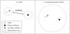 |
Fig. 1 Typical calibration setup for cm VLBI (left) and international LOFAR (right). Note that in some cases the target may itself function as the secondary calibrator. A secondary calibrator is not always required for cm VLBI, but will almost always be needed for international LOFAR, unless the primary calibrator is fortuitously close. The larger field of view of LOFAR means that both the primary and secondary calibrators will always be observed contemporaneously, unlike in cm VLBI, where nodding between the primary calibrator and target is typically required (shown by the double arrow in the left panel). |
To reiterate: in standard VLBI, a primary calibrator is used to solve for the bulk delay and rate offsets in the approximate direction of the target source. Usually this primary calibrator cannot be observed contemporaneously with the target source, and so a nodding calibration is used, where scans on the target are interleaved between scans on the calibrator. Depending on the observing frequency and conditions, and the separation to the primary calibrator, no further refinement may be needed. However, it is common to use a secondary calibrator, or the target itself if bright enough, to derive further phase-only corrections. Naturally, the use of phase-only corrections imposes the requirement that the differential delay between the primary calibrator direction and the target direction be small enough that it can be approximated as a constant phase offset across the width of the primary solution bandwidth. For bandwidths of tens of MHz, this means the differential delay error must be ≲1 ns. Finally, all of the observing bandwidth can be combined to derive these secondary corrections, improving sensitivity.
2.2. Application to LOFAR
For 110–240 MHz (LOFAR high band) observations on long baselines, the approximations made when solving for phase, phase rate, and non-dispersive delay fail badly when applied to bandwidths of tens of MHz or more. Two options present themselves: to add additional parameters (covering dispersive delay and dispersive delay rate) to the global fit, or to reduce the solution bandwidth such that the constant dispersive delay approximation becomes valid again. The former option is obviously preferable from a sensitivity perspective, but greatly expands and complicates the solution search space. Efforts are underway to implement such an expanded fit, including in addition differential Faraday rotation, which becomes increasingly important at frequencies below 100 MHz. First tests on individual long baselines of LOFAR, as well as baselines to other telescopes, are promising, but the algorithms are not yet sufficiently mature for automatic calibration. Accordingly, we focus here on sources that can serve as primary calibrators under the latter set of conditions, where solution bandwidths are limited to no more than a few MHz.
The system equivalent flux density (SEFD) of a single LOFAR core station is approximately 1500 Jy4 at a frequency of ~140 MHz (van Haarlem et al. 2013). An international station has twice the collecting area of a core station at ~140 MHz, so the expected SEFD is around 750 Jy. The 24 core stations can be coherently combined into a single phased array with an SEFD of ~65 Jy, in the absence of correlated noise (i.e. when the observed field only contains sources significantly fainter than the station SEFD). The theoretical 1σ baseline sensitivity of an international station to the phased-up core station, given 3 MHz of bandwidth and four minutes of observing time, is hence 8 mJy in a single polarisation. A source with a compact flux density of 50 mJy yields a theoretical baseline signal-to-noise ratio of 6, and is therefore a potential primary calibrator. In the real world, the sensitivity of the phased-up core station will be reduced by failing tiles, imperfect calibration and correlated (astronomical) noise, and so 50 mJy should be considered a lower limit on the useful primary calibrator flux density.
In addition to being sufficiently bright, the primary calibrator must be close enough to the secondary calibrator and target field that the differential delay between the two fields does not lead to decorrelation when phase-only secondary calibration is performed (just as for cm VLBI). The solution bandwidths are narrower by a factor of ≳10 than for cm VLBI, which is helpful, but the ionospheric delay (inversely proportional to observing frequency squared) is much greater, meaning that on balance a closer calibrator will be needed than the ≲5 degrees typical for cm VLBI. The maximum acceptable separation will be a strong function of ionospheric conditions and elevation, but at face value, given a bandwidth 20 times narrower (e.g. 3 MHz vs. 64 MHz) and frequency 10 times lower (140 MHz vs. 1400 MHz), one would expect that the calibrator would need to be separated by ≲1 degree. This is borne out by commissioning observations with LOFAR, which have shown acceptable results with separations up to several degrees in favourable ionospheric conditions, and unacceptable results with separations as small as ~0.8 degrees in poor conditions. Ideally, then, a primary calibrator for international LOFAR observations would be located ≲1 degree from the secondary calibrator and target field to provide acceptable calibration under most circumstances. As illustrated in Fig. 1, this leads to the one calibration advantage of international LOFAR compared to cm VLBI; since the beam of an international LOFAR station is ≳2 degrees across, the primary calibrator will by necessity be observed contemporaneously with the target source.
This paper focuses on the identification of primary calibrators for high band (110–240 MHz) international LOFAR observations. The reason is that after primary calibration, the bandwidth can be increased by a factor of ~30 for secondary calibration. That means that for target sources brighter than ~10 mJy the target itself can serve as secondary calibrator. Even when the target is not sufficiently bright, the density of these faint sources on the sky is high enough that a suitable calibrator should be found very close to the target. We discuss the identification of secondary calibrators further in Sect. 5.3.
3. Observations and data reduction
When operating in 8-bit mode (van Haarlem et al. 2013), LOFAR has 488 sub-bands of width 0.195 kHz that can be flexibly distributed over a number of beams. For our purposes, a potential calibrator source must be detected within a single 3 MHz band to be useful, so we could divide the available bandwidth over a large number of target sources, enabling rapid surveying.
Log of the observations.
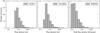 |
Fig. 2 Flux density distribution of the observed sources in the VLSSr catalogue at 74 MHz (left panel, 447 sources), and WENSS at 325 MHz (right panel, 629 sources). The middle panel shows the estimated flux density at 140 MHz interpolated from the two catalogues for sources with counterpart on both catalogues. |
Two hour-long commissioning observations were conducted in May and November 2013, as summarised in Table 2. All available LOFAR stations were utilised: 24 core stations and 13 remote stations in the Netherlands, and 8 international stations (see van Haarlem et al. 2013 for the list and locations of the stations). However, data from some stations were not useful as noted in Table 2. During the first observation, DE604 was using a wrong observation table, whereas for the rest of the stations without valid data a communication problem caused the data to be lost before getting to the correlator in Groningen. Each 1 h observation contained 12 4 min target scans, plus 1 min between scans required for setup. For each target scan, we generated 30 beams to observe simultaneously 30 sources. The tile beam centre was set to the source closest to the centre of the corresponding group, so the 30 sources are within an area of ~2° from the pointing centre. Each beam was allocated with 16 sub-bands with spanned bandwidth of 138.597–141.722 MHz, a frequency range chosen because it is near the peak of the LOFAR sensitivity and is free of strong radio frequency interference (RFI). Additionally, we observed a bright calibrator (3C 380 or 3C 295) for five minutes at the beginning and at the end of each observation. The angular and temporal separation of these scans from the target scans is too large for them to be useful for the international stations, but they are used to calibrate the core and remote stations, and we refer to it hereafter as the “Dutch” calibrator source to distinguish it from the discussion of primary and secondary calibrators for the international stations. The separation between the Dutch calibrator and the targets is 7.5–26° for 3C 380, and 13–22° for 3C 295, for observation 1 and 2, respectively. We note that these separations are predominantly north-south. For the Dutch calibrator scans we used a single beam of 16 sub-bands, spanning the same bandwidth as the target observations.
3.1. Target selection
In our two observations, we applied different selection criteria to cover a wide range of sources that could potentially be useful international LOFAR primary calibrators. The selection was based on the WENSS catalogue (Rengelink et al. 1997). We used the peak flux density of the sources in this catalogue instead of the integrated flux density because with a resolution of 54′′ any extended emission in WENSS will not contribute to the compact flux at ~1″ scales relevant to the LOFAR long-baseline calibration. We note that all WENSS peak flux densities in this paper include a correction factor of 0.9 with respect to the original catalogue to place them in the RCB scale (Roger et al. 1973), as recommended by Scaife & Heald (2012). For the first observation we selected an area of 11.6° radius centred on (18h30m, +65°), or Galactic coordinates (l,b) = (94.84°, + 26.6°). The field contains 9251 sources from the WENSS catalogue (Rengelink et al. 1997) at 325 MHz. We focussed on the brightest sources by randomly selecting 360 of the 1414 sources with a peak flux density above 180 mJy/beam (at the WENSS resolution of 54′′). Ten of the selected sources are also known cm-VLBI calibrators. The second field observed was centred on (15h00m, +70°), or (l,b) = (108.46°, + 43.4°), with a radius of 4.86°. Within this field, we selected any known cm-VLBI calibrators with an integrated VLBI flux density above 100 mJy at 2.3 GHz; there were six such sources. We completed our allocation of 360 sources by selecting all sources with a WENSS peak flux density in the range 72–225 mJy/beam at 325 MHz. In this way, we covered a representative sample of sources with peak flux densities >72 mJy/beam at 325 MHz, including a small sample of sources that were known to be compact at cm wavelengths (the known cm-VLBI calibrators).
Because of a system failure, part of the data were lost during the observations, and two scans (60 sources) were missing during the first observation and one scan (30 sources) was lost during the second observation. Therefore, the actual number of observed sources is 630, with 300 in the first field and 330 in the second.
In Fig. 2 we show the distribution of flux density of the counterparts of the observed sources found in the VLSSr catalogue at 74 MHz, 4 m wavelength (Lane et al. 2012, 2014) and the WENSS catalogue at 325 MHz, 92 cm wavelength. Like the (corrected) WENSS flux densities, the VLSSr catalogue flux scale is also set using the RCB flux density scale (Roger et al. 1973). Based on these two values, we also show the distribution of the estimated flux density of the sources at 140 MHz.
3.2. Data reduction
The data reduction proceeded as follows. First, we performed automathic standard RFI flagging and we averaged the data to a temporal resolution of two seconds and a frequency resolution of 49 kHz (four channels per LOFAR sub-band). Subsequently, we calibrated the complex gains of the core and remote stations using the standard LOFAR tool Black Board Selfcal (BBS; Pandey et al. 2009) on the Dutch array calibrators 3C 380 and 3C 295, using a simple point-source model. We enabled beam calibration, which corrects for the elevation and azimuthal dependence of the station beam pattern in both linear polarisations before solving for complex gain, using a model incorporating the station layout and up-to-date information on station performance, such as failed tiles. To derive the solutions we only used baselines between core and remote stations, rather than core-core or remote-remote baselines. By avoiding the shortest baselines (≲3 km) we ensure that other nearby, bright sources do not contaminate the calibration solutions, while by avoiding the longest baselines (≳55 km) the point-source calibrator model remains valid. Alternatively, all baselines can be used if a detailed model of the structure of the source and all the nearby sources are considered during the calibration.
We derived a single amplitude and phase solution for each sub-band, for each scan on the Dutch array calibrator, and for each of the two observations. We verified that the phase solutions were relatively constant in time for the core stations. BBS does not allow interpolation of solutions, and so we only used the solutions from a single scan (the final scan) to correct the core and remote station gains for the entire dataset. The gains of the international stations were not included in this solution and are left at unity. The solution table was exported with “parmexportcal”5 to be applied to data that were not observed simultaneously to the calibrator. Finally, the solutions were applied to all sources using “calibrate-stand-alone” with a blank model as input. Note that this scheme applies the a priori station beam corrections to all stations (including the international stations); the additional “solved” corrections are present only for the core and remote stations, but not for international stations.
With the core stations now calibrated, it was possible to form a coherent “tied station”, hereafter TS001, from all of the core stations. Because the beams are already centred directly on individual sources, the phasing-up of the core stations does not require additional shifts, which significantly reduces the processing time. We formed TS001 by summing baseline visibilities with the New Default Pre-Processing Pipeline (NDPPP) task “StationAdder”. NDPPP forms a major component of the standard LOFAR imaging pipeline, and is described in Heald et al. (2010) and, with the most up-to-date information, in the LOFAR imaging cookbook (see footnote 5 on page ). After this step, all original visibilities with baselines to core stations were discarded using the NDPPP task “Filter” to reduce data volume.
Subsequently, for each source we combined the 16 sub-bands together into a single measurement set using NDPPP. To avoid the rapid phase changes with frequency introduced into linear polarisation data on long baselines by differential Faraday rotation, we converted the data to circular polarisation with the Table Query Language (TAQL) to operate on the measurement set data directly6. As the effects of the station beam were already calibrated, this is a simple operation. However, we note that since BBS calibrates the XX and YY components independently, an overall phase-offset between X and Y may remain. Although this could not be corrected for this project, we checked that the residual RL and LR leakage is a minor contribution and not critical for this kind of detection experiment. Finally, we converted the measurement set to UVFITS format to proceed with the phase calibration using the AIPS software package (Greisen 2003). At this stage, we had reduced the data volume from the original >4000 GB from a one hour observation to 35 GB, and we had generated a much more sensitive tied-array station to aid the derivation of calibration solutions to the international stations.
In AIPS we conducted a phase calibration by fitting the station-based phases, non-dispersive delays, and rates using the task FRING. We searched solutions using all international stations and the combined core station, TS001, which we used as a reference station. No models were provided for any sources, and hence all sources were assumed to be point-like. The maximum search window for delay and rate was set to 1000 ns and 50 mHz, respectively. These windows were motivated by the largest values expected from ionospheric effects. However, a 1000 ns delay search (or 50 mHz rate search) corresponds to the effect incurred by a source up to 5 arcmin (13 arcmin) away from the nominal position, for the shortest international station to LOFAR core baselines. Confusing sources more than 5 arcmin away from the nominal source direction were therefore filtered out. Additionally, the tied station has a synthesised field of view of about 3 arcmin, and thus sources further away than this distance will contribute less to the fit. We set the solution interval to the scan duration (four minutes), and so only one solution per polarisation was derived per station, per source. We extracted the fit solutions from AIPS for further analysis using the ParselTongue software package (Kettenis et al. 2006).
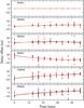 |
Fig. 3 Station delay offsets as a function of time for those sources with fringe solutions for all stations. Up to 30 sources are observed simultaneously at each time interval. The delays are referenced to the average for each station quoted in Table 3. Black circles correspond to left-hand polarisation delays, τL, and red circles correspond to right-hand polarisation delays, τR. The formal uncertainties from the fringe fit are smaller than the markers. |
4. Analysis
With these snapshot observations, it is not possible to conduct an amplitude calibration of the international stations. None of the sources observed have a model that could reasonably be extrapolated to our observing frequency and resolution, and so self-calibration is not feasible. At present, the instrumental gains within LOFAR are not tracked with time7, and so making a sufficiently accurate a priori calibration is also not feasible. With a longer observation (as would be typical for a normal science observation), it would be possible to bootstrap from approximate amplitude corrections for the international stations and image and self-calibrate the target source, but the uv coverage in our snapshot observations is too sparse for such an approach.
Instead, we base our analysis of the compactness of the sources on the phase information of the data, and in particular, on the capability of each source to provide good delay and rate solutions for the international stations. To identify good solutions, we first need to identify an approximation to the true station delay. To accomplish this, we selected only sources that provided delay and rate solutions with a signal-to-noise ratio above six for all stations. In Figs. 3 and 4, we show the evolution of the delay with respect to time. We plot the delay offset with respect to the average value for each station, which is quoted in Table 3. We fitted a polynomial of degree 3 to the delay evolution with time and plotted it using a solid line. We measured the delay rate as the average delay derivative with time for each station. In summary, in Table 3 we quote the average delay per station and polarisation, which is the reference for the offsets in Figs. 3 and 4. We also quote their uncertainties, computed as the standard deviation from the fitted polynomial, and the measured delay rate, computed as the average delay derivative for each station.
Average station-based delay solutions in left (τL) and right (τL) circular polarisation, fitted to the subset of sources which gave good solutions on all stations.
If the model applied at correlation time was perfect, all stations would see a delay offset of zero for all sources, but deviations are produced by several factors. Table 4 summarises the main contributions and the timescale in which they change. First, errors in station positions (and on a much lower level errors in the Earth orientation parameters, EOPs) used by the correlator produce variability of about ±75 ns with a 24 h periodicity. The current correlator model used by LOFAR is insufficiently accurate, and this source of error can be expected to be greatly reduced in the near future. Instabilities in the rubidium clocks can produce delay rates up to 20 ns per 20 min, which corresponds to about a radian per minute at 150 MHz (van Haarlem et al. 2013). In total, non-dispersive instrumental delays of up to ~100 ns and delay rates of up to ~20 ns h-1 are expected. Second, for any given source, errors in the a priori centroid position (which is based on the WENSS position, with a typical error of 1.5′′) and/or extended structure on subarcsecond scales contribute an additional delay offset. The maximum baseline between an international station and the LOFAR core is 700 km (for the FR606 station in France); a positional error of 1.5′′ will lead to a delay error of ~15 ns on this baseline.
Approximate delay contributions at 140 MHz to a 700 km baseline.
The ionospheric contribution to the delay changes as a function of time, position, and zenith angle. The magnitude of the changes depend on the total TEC of the ionosphere, with a delay of τion = c2re/ (2πν2) × TEC, c being the speed of light, re the classical electron radius, and ν the observed frequency. The TEC is usually measured in TEC Units (1TECU = 1016 electrons m-2), and can can be estimated using models derived from observations of GPS satellites. Models are available from different institutes, such as the Jet Propulsion Laboratory (JPL), the Center for Orbit Determination in Europe (CODE), the ESOC Ionosphere Monitoring Facility (ESA), among others. We used the models produced by the Royal Observatory of Belgium GNSS group8, which are focussed in Europe and have an angular resolution of 0.5 degrees and a temporal resolution of 15 min. The models contain information on the vertical total electron content (VTEC) during the two observations, which were conducted shortly after sunrise and at night, respectively. We note that the TEC values above the stations are a lower limit of the slant ionospheric contribution that depends on the source elevation at each station. More details can be found in, for instance, Nigl et al. (2007) and Sotomayor-Beltran et al. (2013).
The VTEC above the international stations was about 12–16 and 4–8 TECU for observation 1 and 2, respectively. These values correspond to an ionospheric delay at 140 MHz of about 850–1100 ns, and 300–540 ns, respectively. These values were approximately constant for observation 2, and were changing at a rate of 90–120 ns h-1 for observation 1. These changes are expected, based on ~0.1–0.2 TECU variations in 10 min seen with the VLA at 74 MHz by Dymond et al. (2011), which corresponds to about 10 ns at 140 MHz. Although all VTEC follow a similar 24 h trend strongly correlated with the Sun elevation, the short-term (10–60 min) variations between the widely separated international stations are virtually uncorrelated. The ionospheric contribution typically dominates the total delay and delay rate for international LOFAR stations. However, for sources observed simultaneously, up to 30 per scan, the ionospheric contribution should be similar because they are separated by 4° at most. We have used VLBI observations (VLBA project code BD152) at 300 MHz, or 1 m wavelength, of bright and compact pulsars at different angular separations to obtain a rough estimate of the delay difference between sources separated 1–5 degrees at elevations of 50–80°. As a first approximation we estimated that the dispersive delay difference between sources at different lines of sight should be about 5 ns per degree of separation for a source elevation of 60°.
Noise is the final contribution to the delay offset, and depends on the brightness of the source and the sensitivity of the station. The dispersions shown in Figs. 3 and 4 are due to source position and structure errors, differential ionosphere, and noise. As shown above, errors of up to several tens of ns can be expected for any individual source from both source position errors and differential ionosphere for our observing setup. In this analysis, we assume that this contribution is random for any given source, and that the delays measured at each time should cluster around the real instrumental + mean ionospheric delay for each station at the time of the scan.
4.1. Quality factor
To complete our analysis, we compute a discrete quality factor, q, for each source, assigning q = 3 to bright and compact sources (i.e. good primary calibrators), q = 2 to partially resolved sources, and q = 1 to resolved or faint sources. The quality factor q is based on how many international stations can be fringe fitted using a particular source to give a satisfactory station delay. A source produces a good delay solution if the fit has a S/N above 6, the difference between right- and left-circular polarisations is below 30 ns, and the deviation from the average delay (see Table 3) is below 300 ns. For each source, the factor q is assigned depending on the number of satisfactory delay solutions found. For an observation with N international stations, q = 3 is assigned if the number of satisfactory delay solutions is ≥ N − 1; i.e. at most one station failed to provide a solution. Failure of only one station is not uncommon on these observations with only one short scan. Sources with q = 3 are almost certainly suitable primary calibrators.
A quality factor q = 1 corresponds to sources with a very low number of good calibrated stations, where the number of failed solutions exceeds 3. These sources are heavily resolved on international LOFAR baselines and are almost certainly unsatisfactory primary calibrators. The intermediate category q = 2 corresponds to sources where a significant number of stations see good solutions, but at least two fail. This group would consist primarily of sources with significant structure on arcsecond scales. Some of these sources may be suitable for calibration if a good model of the source structure could be derived, but many would simply contain insufficient flux density on subarcsecond angular scales. The total number of sources in each group is listed in Table 5.
Number of sources as a function of quality factor.
A catalogue containing the list of sources, basic information in the WENSS, VLSSr, and NVSS catalogues, and the quality factor q obtained here is available in electronic form at the CDS. A sample of some of the columns and rows of the catalogue is shown in Table 6.
Catalogue of observed sources.
5. Results
5.1. Sky distribution
With the selection of good (q = 3) and potentially good (q = 2) primary calibrators for the LOFAR long baselines provided by the international stations, we can study the properties of this source population. In Figs. 5 and 6 we show the distribution of observed sources for observation 1 and 2, respectively, and the corresponding quality factor indicated by the size and colour of the markers. The gap in Fig. 5 in right ascension 17–18 h and declination 60–68° is due to the loss of two scans (60 sources). In the second observation, the sources were distributed in three passes through four different sectors, and thus the loss of one scan only produced a lower number of sources in the north-western sector. The distribution of good sources does not depend on the distance to the Dutch array calibrator, used to phase-up the core stations. Also, no significant bias is seen with respect to right ascension or declination. Therefore, the distribution primary calibrators that are likely to be good (q = 3) is uniform in these two fields.
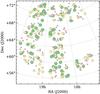 |
Fig. 5 Sky distribution of the sources in observation 1, with markers indicating good primary calibrators, q = 3 (big green circles), potentially good primary calibrators, q = 2 (medium-size yellow circles), and sources that are resolved or faint or both, q = 1 (small red circles). The gap in right ascension 17–18h and declination 60–68° is caused by the failure of two scans, as described in the text. |
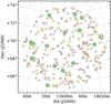 |
Fig. 6 Sky distribution of the sources in observation 2, with markers indicating good primary calibrators, q = 3 (big green circles), potentially good primary calibrators, q = 2 (medium-size yellow circles), and sources that are resolved or faint or both, q = 1 (small red circles). |
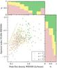 |
Fig. 7 Source quality as a function of low-frequency spectral index and WENSS peak flux density. Red, yellow, and green colours represent q = 1,2, and 3, respectively. q = 3 corresponds to suitable primary calibrators. The histograms show the percentage of sources at each quality value. The histogram on the right does not include the sources with upper limits in their spectral indexes. The uncertainties of some of the values are smaller than the symbols, especially for the WENSS peak flux density. The stripes at low peak flux densities are due to sources detected at multiples of the rms noise of VLSSr. |
5.2. Flux density, spectral index, and extended emission
We used the information in the VLSSr, WENSS, and the NVSS (Condon et al. 1998) surveys to study the correlation of flux density, spectral index, and compactness (as seen from low angular resolution data) with their suitability to be a primary calibrator, as evidenced by the quality q.
To compute the spectral index of the sources, we used the integrated flux density in VLSSr and NVSS, and the peak flux density in WENSS. The three surveys all have different resolutions (75, 45, and 55 arcsec, respectively), which makes a direct comparison of flux density, and hence spectral index, difficult (regardless of whether peak or integrated flux density is used). Fortunately, relatively few sources are resolved in these surveys, and so for each survey we chose to simply use the primary value given in the survey catalogue in question. We do not take into account the small biases that are introduced to the spectral indices measured in this was in the following analysis.
In Fig. 7, we show the distribution of sources as a function of low-frequency spectral index, measured with VLSSr and WENSS, and the peak flux density in WENSS. The histograms show the percentage of sources with each q factor for different ranges of these two variables. We see that brighter sources are more likely to be good primary calibrators, which is not surprising: for a faint source to be a suitable calibrator almost all of the flux density must be contained in a subarcsecond component, whereas a bright source can possess significant extended emission and still contain sufficient flux density in a compact component. Sources that are brighter than 1 Jy/beam at 325 MHz are more likely than not to be a satisfactory primary calibrator, whereas sources of 0.1 Jy/beam are extremely unlikely to be suitable.
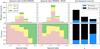 |
Fig. 8 Source quality as a function of low-frequency spectral index (left panel) and high-frequency spectral index (middle panel), with absolute number of sources and percentage at each quality factor. In the right panel we show the number of sources with a given quality showing or not showing a low-frequency turnover. |
Figure 7 also shows that sources with a flatter low-frequency spectrum (measured in this instance from 74 to 325 MHz) are much more likely to be satisfactory primary calibrators. Again, this is unsurprising: steep-spectrum emission is typically associated with extended radio lobes, which would be resolved with our subarcsecond resolution. Sources with a low-frequency spectral index >–0.4 (where S ∝ να) are almost always suitable primary calibrators.
However, the spectral index at higher frequencies (computed in this instance from 325 to 1400 MHz, using WENSS and NVSS) is a much poorer predictor of calibrator suitability. Figure 8 shows the distribution of quality factor with low- and high-frequency spectral index. The lower number of sources with low-frequency spectral index is because fewer sources have a VLSSr counterpart. The difference in predictive power is obvious: by selecting a source with spectral index >–0.6, the chance probability of the source having q = 3 is 51% if we use the low-frequency spectral index, and only 36% if we use the high-frequency spectral index. The right panel of Fig. 8 shows the relative prevalence of a spectral turnover (where the low-frequency spectral index is flatter than the high-frequency spectral index) for the three quality bins. Good primary calibrator sources (q = 3) are more likely to have a spectral turnover.
Total number and percentage of sources as a function of quality factor and source compactness.
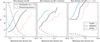 |
Fig. 9 The effect of applying different preselection criteria to improve the detection fraction of calibrator sources, including a lower limit on flux density (left panel), lower limit on flux density plus requiring a low-frequency spectral turnover (middle panel), or lower limit on flux density plus a lower limit to spectral index as calculated between VLSSr and WENSS (right panel). The three colours correspond to imposing the lower flux density limit on the value obtained from VLSSr (orange), WENSS (black), or NVSS (blue). In each panel, the dashed line shows the fraction of the total sample that remains as the lower limit to flux density is raised, while the solid line shows the fraction of that remaining sample that are good calibrators. Imposing a spectral turnover or low-frequency spectral index requirement can reduce the sample size by a factor of 10 whilst still discovering almost half of the total acceptable calibrators. |
Finally, for each source we can check whether it was resolved in the VLSSr and NVSS catalogues. In Table 7 we show the number of sources listed as resolved and unresolved in each catalogue and the associated quality factor percentages. The low angular resolution of VLSSr means that almost all sources in the catalogue are unresolved and few conclusions can be drawn. On the other hand, one-third of the sources in NVSS are resolved by that survey, and we can determine significant trends. If a source is resolved by NVSS, it is very unlikely to be a good primary calibrator (more than five times less likely than if it is unresolved in NVSS). Table 7 also shows the percentage of cm-VLBI calibrators that are compact in our data. Six out of the 15 cm-VLBI calibrators are not good calibrators at 140 MHz, three with q = 1, and three with q = 2. Four of them have inverted or gigahertz peaked spectra and are probably too faint at 140 MHz. The remaining two VLBI sources that proved to be unsatisfactory calibrators, J1722+5856, and J1825+5753, have a flat-spectrum VLBI core with moderate flux density (~150–200 mJy); they may have decreased in flux density since the VLBI observations, or possibly the core exhibits a low-frequency turnover. Based on our small sample of cm-VLBI calibrators, compactness at cm wavelengths is also a good predictor of suitability as an international LOFAR primary calibrator. A sufficiently bright cm-VLBI calibrator, accounting for spectral index, will have enough compact flux at 140 MHz with very high reliability. Although the correlation between being a cm-VLBI calibrator and being a good LOFAR calibrator is clear from these data, we note that this conclusion relies on a very low number of sources (15) and more observations would be needed to derive more accurate statistics.
5.3. Calibrator selection strategies and sky density
We have shown above that peak flux density, low-frequency spectral index, and compactness on scales of tens of arcsec are all good predictors of primary calibrator suitability for LOFAR. To help select a sample of potential calibrators, in Fig. 9 we plotted the percentage of good primary calibrators, with q = 3, as a function of the minimum peak flux density imposed to the sample, for three different selection criteria. For example, the left panel shows that we expect 20% of the sources with WENSS peak flux density above 0.2 Jy/beam to be good primary calibrators. If we additionally impose that the sources have a low-frequency turnover (middle panel) then the probability of having a good source increases to 45%, whereas selecting sources with flat low-frequency spectrum (right panel) increases the chances to 50%. However, a restrictive criterion comes with a reduction of the number of sources in the sample, as shown by the dashed lines. The low number of sources in the right panel compared to the middle panel is also because many of the faint sources are not detected with VLSSr. Thus, a measurement of the spectral index is not available, although it is still possible to infer that there is a turnover when the source is not detected.
However, rigorous preselection is unlikely to be necessary in practice. Based on these results, we can extrapolate to the density of suitable primary calibrators on the sky. The field observed in the first epoch contains 1200 WENSS sources with peak flux density above 180 mJy/beam, from which we observed 300 and found 70 good primary calibrators, giving an estimate of 280 good calibrators in the effective 350 square degrees observed. Therefore, the density of good primary calibrators for the criteria of epoch 1 is 0.8 per square degree. The 16 good primary calibrators, out of 330 sources with WENSS peak flux densities between 72 and 225 mJy/beam found in the 62 square degrees of observation 2, provide 0.24 good primary calibrators per square degree. To obtain the density of the whole sample, we corrected for the sources being counted twice in the same flux density range: WENSS peak flux densities between 180 and 225 mJy/beam. We conclude that the density of good primary calibrators with 325 MHz peak flux density >72 mJy/beam is approximately 1.0 per square degree. Unfortunately, the low statistics of the overlap region, with three and four good primary calibrators, respectively, prevents us from obtaining a significant uncertainty on this density.
From the WENSS survey, there are ~7.6 sources above 72 mJy/beam per square degree, 14% of them expected to be good primary calibrators. After an overhead of four minutes for the calibration of the LOFAR core stations, we can survey 30 sources per four additional minutes. That means an area covering 3 square degrees (a radius of ~1°) around a target source can be inspected for primary calibrators in just ten minutes. Without any other preselection, the likelihood of identifying at least one usable calibrator among 30 WENSS sources is 98.9%. Depending on the specific requirements of a project and the characteristics of the field around the target source, this probability can be increased by observing 60 sources up to 1.6° around the target in 15 min, or by setting additional selection criteria (see Fig. 9 or Table 7). This type of calibrator search could easily be undertaken in the weeks prior to a science observation.
Once a primary calibrator has been identified, a secondary phase calibrator closer to the target could be identified if the target itself is not be strong enough for self-calibration. This is more efficiently conducted in a separate, second observation because the full bandwidth would be required to search for fainter sources. This could be set up in an identical manner to a typical international LOFAR science observation, with the pointing centre set to be midway between the primary calibrator and the target field. After correlation, the full-resolution visibility dataset can be shifted and averaged multiple times to the position of the primary calibrator and to the position of all candidate secondary calibrator sources. Since 30× more bandwidth is used, again a ten minute observation would suffice to identify useful secondary calibrators (those with a peak flux density ≳5 mJy/beam).
As an alternative to a separate, short observation before the science observation, a small subset of the data from the science observation itself could be used to search for a secondary calibrator. The advantage of a short search in advance is that the secondary calibrator-target separation is known, which could inform the selection of observing conditions. If a good calibrator is present, poorer quality ionospheric conditions could be tolerated, for instance.
Additionally, the same approach used for finding and using secondary calibrators can be applied several times towards different sky directions to survey the whole station beam. Relatively faint secondary calibrators are expected to be found nearly anywhere in the sky, so the full-resolution dataset can be shifted (and averaged) to a number of different regions within the station beam. The data from the core and remote stations can be used to explore the potential calibrators and targets in the field at low resolution, and the full-array data would improve the sensitivity and the resolution of the survey. Eventually, a full-resolution image of the whole primary beam can be produced, at the expense of a very high computational cost.
We found a density of ~1 good calibrator per square degree based on two fields with Galactic latitudes of + 26.6° and + 43.4°. However, we expect less compact sources at lower Galactic latitudes because of interstellar scattering. The Galactic electron density model NE2001 (Cordes & Lazio 2002) predicts scattering at a Galactic latitude of 50° of almost 100 mas at 150 MHz, which is five times smaller than our resolution. However, the scattering is about 300 mas, similar to our beamsize, at latitudes of 5–10°, depending on the longitude. Therefore, observations below a Galactic latitude of 10° are likely to be affected by scattering on the longest baselines, and the effect should be severe below about 2°, especially towards the Galactic Center. Therefore, an accurate analysis of the area, and a more exhaustive search of calibrators, is required when observing low Galactic latitudes because the compactness of sources can be significantly worse than for the cases presented here.
6. Conclusions
We have observed 630 sources in two fields with the LOFAR international stations to determine the density of good long-baseline calibrators in the sky. We have seen that a number of properties from lower angular resolution data are correlated with the likelihood of being a suitable calibrator. High flux density, a flat low-frequency spectrum, and compactness in the NVSS catalogue are all useful predictors of calibrator suitability. The spectral index at higher frequency, in contrast, is a poor predictor.
The conclusions of this study are:
-
1.
With a survey speed of ~360 targets per hour in “snapshot” surveymode, identifying the optimal calibrator for an internationalLOFAR observation can be inexpensively performed before themain observation.
-
2.
The density of suitable calibrators for international LOFAR observations in the high band (~140 MHz) is around 1 per square degree, which is high enough that a suitable calibrator should be found within 1° of the target source virtually anywhere in the sky (excluding regions of high scattering such as the Galactic plane).
The Multifrequency Snapshot Sky Survey (MSSS) is the first northern-sky LOFAR imaging survey between 30 and 160 MHz (Heald & LOFAR Collaboration 2014) with a 90% completeness of 100 mJy at 135 MHz. It provides low-resolution images and source catalogues including detailed spectral information. At the time of publication, the final catalogue was not available, so it was not included in our analysis. The MSSS catalogue can be used to improve the selection of potential long baseline calibrators.
Finally, we anticipate extending this work in the future with observations at lower frequencies (the LOFAR low band is capable of observing from 15–90 MHz), although the density of suitable sources is expected to be much lower because of the lower sensitivity in this frequency range, combined with an even greater impact of ionospheric conditions.
An up-to-date map of all LOFAR stations can be found at http://www.astron.nl/~heald/lofarStatusMap.html
A secondary calibrator is often referred to as an “in-beam” calibrator if it is close enough to the target source to be observed contemporaneously.
A LOFAR core station consists of two sub-stations (2 × 24 tiles) in the HBA.
A measurement set can be converted to circular polarisation using: update ⟨filename.ms⟩ set DATA = mscal.stokes(DATA,“circ”) and update ⟨filename.ms⟩/POLARIZATION set CORRTYPE = [5,6,7,8].
This is planned to change with the new “COBALT” correlator recently commissioned.
Acknowledgments
LOFAR, the Low Frequency Array designed and constructed by ASTRON, has facilities in several countries that are owned by various parties (each with their own funding sources), and that are collectively operated by the international LOFAR Telescope (ILT) foundation under a joint scientific policy. A.T.D. is supported by a Veni Fellowship from NWO. A.D.K. acknowledges support from the Australian Research Council Centre of Excellence for All-sky Astrophysics (CAASTRO), through project number CE110001020. LKM acknowledges financial support from NWO Top LOFAR project, project n. 614.001.006. CF acknowledges financial support by the Agence Nationale de la Recherche through grant ANR-09-JCJC-0001-01.
References
- Ananthakrishnan, S., Kulkarni, V. K., Ponsonby, J. E. B., et al. 1989, MNRAS, 237, 341 [NASA ADS] [CrossRef] [Google Scholar]
- Clark, T. A., Erickson, W. C., Hutton, L. K., et al. 1975, AJ, 80, 923 [NASA ADS] [CrossRef] [Google Scholar]
- Condon, J. J., Cotton, W. D., Greisen, E. W., et al. 1998, AJ, 115, 1693 [NASA ADS] [CrossRef] [Google Scholar]
- Cordes, J. M., & Lazio, T. J. W. 2002 [arXiv:astro-ph/0207156] [Google Scholar]
- Dymond, K. F., Watts, C., Coker, C., et al. 2011, Radio Science, 46, 5010 [NASA ADS] [CrossRef] [Google Scholar]
- Falcke, H., Körding, E., & Nagar, N. M. 2004, New A Rev., 48, 1157 [Google Scholar]
- Greisen, E. W. 2003, Information Handling in Astronomy – Historical Vistas, 285, 109 [NASA ADS] [CrossRef] [Google Scholar]
- Heald, G., & LOFAR Collaboration 2014, AAS Meet. Abstracts, 223, 236.07 [Google Scholar]
- Heald, G., McKean, J., Pizzo, R., et al. 2010, Proc. ISKAF2010 Science Meeting, PoS(ISKAF2010) 057 [Google Scholar]
- Kettenis, M., van Langevelde, H. J., Reynolds, C., & Cotton, B. 2006, in Astronomical Data Analysis Software and Systems XV, eds. C. Gabriel, C. Arviset, D. Ponz, & S. Enrique, ASP Conf. Ser., 351, 497 [Google Scholar]
- Lane, W. M., Cotton, W. D., Helmboldt, J. F., & Kassim, N. E. 2012, Radio Science, 47, [Google Scholar]
- Lane, W. M., Cotton, W. D., van Velzen, S., et al. 2014, MNRAS, 440, 327 [NASA ADS] [CrossRef] [Google Scholar]
- Lenc, E., Garrett, M. A., Wucknitz, O., Anderson, J. M., & Tingay, S. J. 2008, ApJ, 673, 78 [NASA ADS] [CrossRef] [Google Scholar]
- Nigl, A., Zarka, P., Kuijpers, J., et al. 2007, A&A, 471, 1099 [NASA ADS] [CrossRef] [EDP Sciences] [Google Scholar]
- Pandey, V. N., van Zwieten, J. E., de Bruyn, A. G., & Nijboer, R. 2009, in The Low-Frequency Radio Universe, eds. D. J. Saikia, D. A. Green, Y. Gupta, & T. Venturi, ASP Conf. Ser., 407, 384 [Google Scholar]
- Rampadarath, H., Garrett, M. A., & Polatidis, A. 2009, A&A, 500, 1327 [NASA ADS] [CrossRef] [EDP Sciences] [Google Scholar]
- Rengelink, R. B., Tang, Y., de Bruyn, A. G., et al. 1997, A&AS, 124, 259 [NASA ADS] [CrossRef] [EDP Sciences] [Google Scholar]
- Roger, R. S., Costain, C. H., & Bridle, A. H. 1973, AJ, 78, 1030 [NASA ADS] [CrossRef] [Google Scholar]
- Scaife, A. M. M., & Heald, G. H. 2012, MNRAS, 423, L30 [NASA ADS] [CrossRef] [Google Scholar]
- Sotomayor-Beltran, C., Sobey, C., Hessels, J. W. T., et al. 2013, A&A, 552, A58 [NASA ADS] [CrossRef] [EDP Sciences] [Google Scholar]
- van Haarlem, M. P., Wise, M. W., Gunst, A. W., et al. 2013, A&A, 556, A2 [NASA ADS] [CrossRef] [EDP Sciences] [Google Scholar]
- Vandenberg, N. R., Clark, T. A., Erickson, W. C., Resch, G. M., & Broderick, J. J. 1976, ApJ, 207, 937 [NASA ADS] [CrossRef] [Google Scholar]
- Varenius, E., Conway, J. E., Martí-Vidal, I., et al. 2015, A&A, in press, DOI: 10.1051/0004-6361/201425089 [Google Scholar]
- Walker, R. C. 1999, in Synthesis Imaging in Radio Astronomy II, eds. G. B. Taylor, C. L. Carilli, & R. A. Perley, ASP Conf. Ser., 180, 433 [Google Scholar]
- Wrobel, J. M., & Simon, R. S. 1986, ApJ, 309, 593 [NASA ADS] [CrossRef] [Google Scholar]
- Wucknitz, O. 2010a, in 10th European VLBI Network Symposium and EVN Users Meeting: VLBI and the New Generation of Radio Arrays [Google Scholar]
- Wucknitz, O. 2010b, Proc. ISKAF2010 Science Meeting, PoS(ISKAF2010) 058 [Google Scholar]
Appendix A: How to plan an international LOFAR observation
Given our ability to find and calibrate potential delay calibrators, we propose the following approach for an international LOFAR observation:
-
1.
Identify candidate primary calibrators up to separations of afew degrees by using any of the criteria discussed inSect. 5;
-
2.
Conduct a short observation in snapshot mode as described in Sect. 3 before the science observation to identify the best primary calibrator (or calibrators);
-
3.
If required and time permits, follow up with a “full bandwidth” snapshot observation to identify one or more secondary calibrators;
-
4.
Set up the scientific observation to dwell on the field containing the primary calibrator and the target and secondary calibrator;
-
5.
Include periodic scans (every ~h) on a bright Dutch array calibrator to calibrate the core stations in order to form the tied station;
-
6.
Shift phase centre to primary calibrator, preprocess, and obtain delay solutions as described in this paper, and apply them to the unshifted dataset;
-
7.
If a secondary calibrator is to be used and is not yet identified, select ten minutes of data and perform shift and averaging to candidate secondary calibrator sources;
-
8.
If secondary calibrator is used: shift and average primary-calibrated dataset, image, and selfcalibrate, and apply solutions to the unshifted dataset;
-
9.
Shift and average calibrated dataset, image, and (if needed) selfcalibrate target.
In the near future, the pipeline used for this project will be developed, in collaboration with the LOFAR operations team, into an expanded form capable of carrying out the approach described above. This pipeline will be made available to all international LOFAR observers, delivering a reduced data volume for long-baseline observations and enabling calibrated data to be produced more quickly.
All Tables
Average station-based delay solutions in left (τL) and right (τL) circular polarisation, fitted to the subset of sources which gave good solutions on all stations.
Total number and percentage of sources as a function of quality factor and source compactness.
All Figures
|
Fig. 1 Typical calibration setup for cm VLBI (left) and international LOFAR (right). Note that in some cases the target may itself function as the secondary calibrator. A secondary calibrator is not always required for cm VLBI, but will almost always be needed for international LOFAR, unless the primary calibrator is fortuitously close. The larger field of view of LOFAR means that both the primary and secondary calibrators will always be observed contemporaneously, unlike in cm VLBI, where nodding between the primary calibrator and target is typically required (shown by the double arrow in the left panel). |
| In the text | |
|
Fig. 2 Flux density distribution of the observed sources in the VLSSr catalogue at 74 MHz (left panel, 447 sources), and WENSS at 325 MHz (right panel, 629 sources). The middle panel shows the estimated flux density at 140 MHz interpolated from the two catalogues for sources with counterpart on both catalogues. |
| In the text | |
|
Fig. 3 Station delay offsets as a function of time for those sources with fringe solutions for all stations. Up to 30 sources are observed simultaneously at each time interval. The delays are referenced to the average for each station quoted in Table 3. Black circles correspond to left-hand polarisation delays, τL, and red circles correspond to right-hand polarisation delays, τR. The formal uncertainties from the fringe fit are smaller than the markers. |
| In the text | |
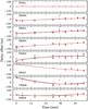 |
Fig. 4 Same as Fig. 3, except for the second observation. |
| In the text | |
|
Fig. 5 Sky distribution of the sources in observation 1, with markers indicating good primary calibrators, q = 3 (big green circles), potentially good primary calibrators, q = 2 (medium-size yellow circles), and sources that are resolved or faint or both, q = 1 (small red circles). The gap in right ascension 17–18h and declination 60–68° is caused by the failure of two scans, as described in the text. |
| In the text | |
|
Fig. 6 Sky distribution of the sources in observation 2, with markers indicating good primary calibrators, q = 3 (big green circles), potentially good primary calibrators, q = 2 (medium-size yellow circles), and sources that are resolved or faint or both, q = 1 (small red circles). |
| In the text | |
|
Fig. 7 Source quality as a function of low-frequency spectral index and WENSS peak flux density. Red, yellow, and green colours represent q = 1,2, and 3, respectively. q = 3 corresponds to suitable primary calibrators. The histograms show the percentage of sources at each quality value. The histogram on the right does not include the sources with upper limits in their spectral indexes. The uncertainties of some of the values are smaller than the symbols, especially for the WENSS peak flux density. The stripes at low peak flux densities are due to sources detected at multiples of the rms noise of VLSSr. |
| In the text | |
|
Fig. 8 Source quality as a function of low-frequency spectral index (left panel) and high-frequency spectral index (middle panel), with absolute number of sources and percentage at each quality factor. In the right panel we show the number of sources with a given quality showing or not showing a low-frequency turnover. |
| In the text | |
|
Fig. 9 The effect of applying different preselection criteria to improve the detection fraction of calibrator sources, including a lower limit on flux density (left panel), lower limit on flux density plus requiring a low-frequency spectral turnover (middle panel), or lower limit on flux density plus a lower limit to spectral index as calculated between VLSSr and WENSS (right panel). The three colours correspond to imposing the lower flux density limit on the value obtained from VLSSr (orange), WENSS (black), or NVSS (blue). In each panel, the dashed line shows the fraction of the total sample that remains as the lower limit to flux density is raised, while the solid line shows the fraction of that remaining sample that are good calibrators. Imposing a spectral turnover or low-frequency spectral index requirement can reduce the sample size by a factor of 10 whilst still discovering almost half of the total acceptable calibrators. |
| In the text | |
Current usage metrics show cumulative count of Article Views (full-text article views including HTML views, PDF and ePub downloads, according to the available data) and Abstracts Views on Vision4Press platform.
Data correspond to usage on the plateform after 2015. The current usage metrics is available 48-96 hours after online publication and is updated daily on week days.
Initial download of the metrics may take a while.