| Issue |
A&A
Volume 574, February 2015
|
|
|---|---|---|
| Article Number | A11 | |
| Number of page(s) | 11 | |
| Section | Extragalactic astronomy | |
| DOI | https://doi.org/10.1051/0004-6361/201424962 | |
| Published online | 16 January 2015 | |
MUSE integral-field spectroscopy towards the Frontier Fields cluster Abell S1063
I. Data products and redshift identifications
1 Kapteyn Astronomical Institute, University of Groningen, Postbus 800, 9700 AV Groningen, The Netherlands
e-mail: karman@astro.rug.nl
2 Dark Cosmology Centre, Niels Bohr Institute, University of Copenhagen, Juliane Maries Vej 30, 2100 Copenhagen, Denmark
3 INAF–Osservatorio Astronomico di Trieste, via G. B. Tiepolo 11, 34143, Trieste, Italy
4 Dipartimento di Fisica e Scienze della Terra, Università degli Studi di Ferrara, via Saragat 1, 44122 Ferrara, Italy
5 INAF–Bologna Astronomical Observatory, via Ranzani 1, 40127 Bologna, Italy
6 Space Telescope Science Institute, 3700 San Martin Drive, MD 21208 Baltimore, USA
7 European Southern Observatory, Alonso de Córdova 3107, Vitacura, Casilla 19001 Santiago 19, Chile
8 Dipartimento di Fisica, Università degli Studi di Milano, via Celoria 16, 20133 Milano, Italy
9 INAF–Osservatorio Astronomico di Capodimonte, Via Moiariello 16, 80131 Napoli, Italy
10 Max-Planck-Institut für Astronomie, Königstuhl 17, 69117 Heidelberg, Germany
Received: 11 September 2014
Accepted: 13 October 2014
We present the first observations of the Frontier Fields cluster Abell S1063 taken with the newly commissioned Multi Unit Spectroscopic Explorer (MUSE) integral field spectrograph. Because of the relatively large field of view (1 arcmin2), MUSE is ideal to simultaneously target multiple galaxies in blank and cluster fields over the full optical spectrum. We analysed the four hours of data obtained in the science verification phase on this cluster and measured redshifts for 53 galaxies. We confirm the redshift of five cluster galaxies, and determine the redshift of 29 other cluster members. Behind the cluster, we find 17 galaxies at higher redshift, including three previously unknown Lyman-α emitters at z> 3, and five multiply-lensed galaxies. We report the detection of a new z = 4.113 multiply lensed galaxy, with images that are consistent with lensing model predictions derived for the Frontier Fields. We detect C iii], C iv, and He ii emission in a multiply lensed galaxy at z = 3.116, suggesting the likely presence of an active galactic nucleus. We also created narrow-band images from the MUSE datacube to automatically search for additional line emitters corresponding to high-redshift candidates, but we could not identify any significant detections other than those found by visual inspection. With the new redshifts, it will become possible to obtain an accurate mass reconstruction in the core of Abell S1063 through refined strong lensing modelling. Overall, our results illustrate the breadth of scientific topics that can be addressed with a single MUSE pointing. We conclude that MUSE is a very efficient instrument to observe galaxy clusters, enabling their mass modelling, and to perform a blind search for high-redshift galaxies.
Key words: gravitational lensing: strong / techniques: imaging spectroscopy / galaxies: clusters: individual: Abell S1063 / galaxies: evolution / galaxies: high-redshift / galaxies: distances and redshifts
© ESO, 2015
1. Introduction
Spectroscopic studies of high-redshift (z> 2) galaxies provide very valuable information on the mechanisms for galaxy growth and evolution in the young Universe. Multiple spectroscopic campaigns targeting high-z galaxies have now been carried out, shedding light on general star formation properties (e.g. Shapley et al. 2003; Kajisawa et al. 2010; Le Fèvre et al. 2013), chemical composition (e.g. Erb et al. 2006a; Maier et al. 2014), and the presence of gas outflows (e.g. Erb et al. 2006b; Steidel et al. 2010; Hainline et al. 2011; Talia et al. 2012; Karman et al. 2014). The search for Lyman-α emitters has also allowed the existence of multiple galaxy candidates at very high-z to be confirmed (z> 5; Pentericci et al. 2011; Stark et al. 2011; Curtis-Lake et al. 2012; Shibuya et al. 2012; Finkelstein et al. 2013; Guaita et al. 2013).
A next, more challenging step is obtaining spectral information coupled to spatial information within each galaxy, through integral field spectroscopy (IFS). Integral field spectroscopy studies have been shown to be very important for revealing the dynamics of star formation in galaxies at z ~ 1 − 2 (e.g. Förster Schreiber et al. 2006; Epinat et al. 2009; Contini et al. 2012), but only a few attempts have so far been possible at higher redshifts (e.g. Mannucci et al. 2009; Blanc et al. 2011). The main reason for this limitation is that the surface brightness of galaxies decreases with (1 + z)4, and thus IFS observations of high-z galaxies with current telescopes require very long exposure times.
Lensing cluster fields are ideal to overcome this limitation, and provide an excellent tool to investigate the high-redshift Universe. In particular, the Hubble Space Telescope (HST) multi-cycle treasury programme CLASH (Postman et al. 2012) has provided deep images over 16 wavebands for 25 cluster fields, enabling a series of photometric studies to identify high-z galaxy candidates (Jouvel et al. 2014; Monna et al. 2014; Vanzella et al. 2014), and model in detail the lensing properties of such systems (Coe et al. 2012; Zitrin et al. 2013; Grillo et al. 2014a). A major spectroscopic follow-up of a subset of these clusters is currently in progress with the VIsible MultiObject Spectrograph (VIMOS) at the Very Large Telescope (VLT), in the so-called CLASH-VLT large programme (P.I.: P. Rosati), which has already yielded spectroscopic confirmation of a z> 6 galaxy candidate (Balestra et al. 2013; Richard et al. 2014a; Johnson et al. 2014), and allowed for more accurate lensing models for some of these clusters (Biviano et al. 2013; Grillo et al. 2014b).
With the aim of investigating one of these cluster fields in further detail, we carried out the follow-up of Abell S1063 (RXCJ2248.7-4431) with the new Multi Unit Spectroscopic Explorer (MUSE) IF spectrograph on the VLT (Bacon et al. 2010). Abell S1063 is one of the four CLASH lensing clusters that was selected for ultra-deep observations as part of the HST Frontier Fields programme (Lotz et al., in prep.). As a pilot programme, we obtained medium-depth data from MUSE over a single pointing covering ~ 1 × 1 arcmin2, with 4 h observations carried out in the MUSE science verification phase. A main aim of this paper is thus to assess the performance of MUSE on a number of science cases.
The layout of this paper is as follows. In Sect. 2 we give a brief overview of the MUSE performance and the obtained data, followed by the data reduction process. In Sect. 3, we describe the obtained spectroscopic results, including the determined redshifts and emission line properties. We give details of narrow-band images constructed from the MUSE data in Sect. 4 to search for weaker sources, and we summarise and discuss our findings in Sect. 5.
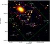 |
Fig. 1 Red-green-blue image composition of HST images of the part of AS1063 that we observed with MUSE, where the colours in this image are blue = F435W + F475W, green = F606W + F625W + F775W + F814W + F850LP, red = F105W + F110W + F140W + F160W. The individual HST images were obtained and distributed by the CLASH collaboration. The green square delimits the 1 × 1′ MUSE FOV. All 19 objects with a spectroscopic redshift z> 1 are shown as white circles and their redshifts. Numbered galaxies were noted before by Monna et al. (2014) and Balestra et al. (2013). The blue, magenta, and red contours correspond to regions where the magnification is μ> 200 at z = 1, 2, and 4, respectively. The magnifications are based on the second version of the Sharon models (Johnson et al. 2014), which were chosen for illustrative purposes, but we note that this is only one out of many different available models. |
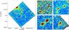 |
Fig. 2 Snapshot of our MUSE pointing towards Abell S1063. Left: a slice of reduced MUSE data cube centred at 7250 Å with Δλ = 1.25 Å. Right: zoom-ins of the four regions with LAEs marked on the left panel, where the wavelength is centred at the peak of Lyαfor galaxies 53a,c 52a,b, 49a,b, and 50 in panels A, B, C, and D, respectively. In zoom-in A, we placed a circle around the weak additional detection of the quintiply lensed galaxy at z = 6.107. |
2. Observations
MUSE is the newly installed integral field (IF) spectrograph on the VLT at the Paranal Observatory (Bacon et al. 2012). The spectrograph has a wide wavelength coverage from 4800 through 9300 Å in the nominal mode, with an average resolution of R ~ 3000. MUSE’s field of view (FOV) is of ~1 arcmin2, and therefore, MUSE combines a high spatial resolution with a large FOV, resulting in more spectral pixels (spaxels) than any other optical IF spectrograph. Because of the relatively large FOV size, MUSE is very well suited to simultaneously target multiple background galaxies in blank and cluster fields. This capability is further improved by its high spatial resolution (0.2′′ pixel scale), which also allows for detailed spatial profiles of the galaxies, and is only limited by seeing until adaptive optics becomes available.
We observed the cluster Abell S1063 with a pointing centred at α = 22:48:42.217, δ = −44:32:16.850, see Fig. 1. We set the position angle to 41° in order to cover the area with maximum magnification according to the CLASH lensing models distributed for the Frontier Fields. Furthermore, this position angle and centre maximises the number of high-redshift candidates and lensed objects as obtained from Monna et al. (2014) and the CLASH Image Pipeline.
Our MUSE observations were carried out as part of the science verification phase of MUSE in the nights of June 25th 2014 (2 × 1420 s) and June 29th 2014 (6 × 1420 s). The 1 h of observations on the 25th were carried out with a seeing of 1′′, while the 3 h of observations on the 29th had a seeing of 1.1′′. We applied a dither pattern consisting of a positional offset and a rotation in our observation strategy to better remove cosmic rays and to obtain a better noise map. The positional offset consisted of a shift of the centre by 0.4−0.8′′, so that every exposure had a slightly different centre. In addition, we rotated every exposure by 90°, resulting in two exposures for every position angle.
2.1. Data reduction
We reduced the raw data using the MUSE data reduction software version 0.18.2, which contains all standard reduction procedures. We show a slice of the resulting datacube in Fig. 2. The pipeline subtracts the bias, applies a flatfielding and calibrates the wavelength by using more than 70 arc lamp lines distributed over the whole wavelength range. The wavelength solution is recalibrated using the atmospheric sky lines in the science exposures. We checked the wavelength and tracing solutions for every IFU and slice, and verified that the residuals were typically < 0.15 Å. For two out of the eight exposures, we removed one slice from one IFU (15″ × 0.2″ spatially) as the detector did not work well in this slice for temperatures below 7 degrees Celsius, and the tracing and flatfielding recipes fail. This is consistent with findings of preliminary MUSE testing (E. Valenti, priv. comm.), and has now been corrected. As a last step, the pipeline calibrates the flux in the exposures using a standard star, and combines all exposures into one 3D datacube, where differential atmospheric diffraction is taken into account. Although the pipeline corrects the data for a small number of telluric lines, many atmospheric lines are still present in the data. We masked the strongest lines in the data manually, but kept the weaker ones, as the data at these wavelengths can still provide useful information when observing emission lines.
To remove cosmic rays from the data, we applied the Python routine of LA Cosmic (van Dokkum 2001) to the raw science data frames, in addition to the cosmic ray removal available in the pipeline. Because the sky is not completely removed from the datacube, we created a mask consisting of eleven regions free of sources, and subtracted the mean of these regions at each wavelength. We identified sources from this sky-subtracted datacube by careful visual inspection, and used the Common Astronomical Software Application (CASA) package1 to collapse the data in the spatial directions within a fitted ellipse and extract 1D spectra. The astrometry was assigned using the distributed astrometry table. To test the positional accuracy, we used the HST images for Abell S1063 as reference. We created three narrowband images with the MUSE observations using the pipeline, and ran Sextractor (Bertin & Arnouts 1996) on both sets of images. We found a median positional accuracy of 0.12″ for MUSE compared to HST.
Fumagalli et al. (2014) found that they needed to rescale the illumination in every slice to properly reduce the data. In addition, they manually created a sky model to subtract from the intermediately produced so-called pixtables to improve the signal. We developed Python routines to perform similar steps in our data reduction, but we do not find a substantial improvement to the quality of our data. Therefore, we do not use the data reduced with these illumination or sky corrections in this paper.
Figure 2 shows the reduced MUSE data at 7250 Å. A large number of sources and the overall good data quality are clearly evident from Fig. 2.
3. Spectral analysis
We extracted 1D spectra for 61 detections, belonging to 53 individual galaxies, in our observed 1 arcmin2 field, and determined their redshifts, see Tables 1 and 2. Of these objects, 34 are galaxies within 5000 km s-1 of the cluster redshift (zc = 0.348Böhringer et al. 2004; Guzzo et al. 2009), 25 detections correspond to 17 individual galaxies at higher redshift, and 2 are foreground galaxies. We find five more objects with spectral features that are too weak to securely determine a redshift.
3.1. Cluster galaxies
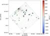 |
Fig. 3 Distribution map of the identified cluster galaxies. Squares correspond to passive galaxies, while stars indicate active galaxies, where their classification is based on the presence or absence of optical emission lines. The galaxies have been coloured according to their velocity relative to the cluster, with bluer colours meaning higher velocities towards us, and redder colours corresponding to higher velocities away from us. |
Properties of the detected cluster galaxies in the observed field.
We show the properties of the cluster galaxies in Table 1. We note that only five of the determined cluster galaxies have a previously published redshift determination (Gómez et al. 2012), and therefore we add redshifts to 29 galaxies of the cluster. The redshift measured for the cluster galaxies is in excellent agreement with measurements from VIMOS (Balestra et al., in prep.). We find that almost all the cluster galaxies have very similar spectra. In all 34 galaxies we detect Ca ii H and K, and 33 show a strong 4000 Å break. We used the presence or absence of the [O ii] λλ 3726.0,3728.8 Å, H β, [O iii] λ 5006.8 Å, and H α to classify the cluster galaxies as active if we find at least one these lines with a negative equivalent width, i.e. it is in emission, or passive otherwise. Out of the 34 galaxies, only two are classified as active, while the remaining 32 are all lacking signatures of activity. The classification active does not distinguish between star formation activity and AGN, as we do not determine the ionizing source. We show the distribution of the cluster galaxies in Fig. 3 in which we also indicate their classification. It is clear from this figure that the number density of cluster members increases towards the centre of the cluster, and that almost all bright objects with a visible continuum are part of the cluster. The two active galaxies do not appear to be at the cluster outer regions, as would be expected if they were recently accreted by the cluster. However, because this only involves two galaxies, this could well be due to projection effects.
In Figs. 4 and 5 we show two example spectra of bright cluster galaxies to illustrate the spectral properties. Figure 4 shows the spectrum of object 2. We see a bright continuum, with two strong absorption lines between 5220 and 5320 Å, identified as the Ca ii H and K lines. Furthermore, we see a clear absorption feature at the G-band, and all Balmer lines are in absorption. Absorption of the Mg i line at 5175 Å rest frame also indicates an old stellar population and is clearly visible in the spectrum. In agreement with the purely old population, there are no emission lines visible over the whole wavelength range.
Object 9, Fig. 5, shows strong absorption lines around 4000 Å, easily recognisable as the Ca ii and H δ lines. The 4000 Å break is clear, and we see a small but broad absorption corresponding to H β. Although all of these properties indicate that the stellar population is old, we find some [O ii] λλ 3726.0, 3728.8 Å and clear [N ii] λ6585 Å emission. Because there is no [O iii] emission visible, it is unlikely that an AGN is responsible for the [O ii] emission, as AGN have a higher ionisation level. Post-starburst galaxies sometimes show weak [O ii] emission, however, the H δ equivalent width measured for this object, EW ≈ 0.5 Å, is significantly less than the EW = 3 − 5 Å observed in post-starburst galaxies. Therefore, we conclude that this emission of [O ii] indicates a young stellar population coexisting with the underlying old stellar population.
We show the spectrum of one cluster galaxy (object 5) classified as active in Fig. 6. There is no clear continuum recognised by visual inspection for this source, but we do see several emission lines, including [O ii], H γ, H β, and [O iii]. The only strong emission line that we do not detect is H α, as it is hidden behind a skyline. However, we see a weak signal at the red side of the skyline, indicating that the H α line may also be strong. When spatially collapsing the data, we see that a continuum is visible, including the strongest absorption features.
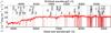 |
Fig. 4 Spectrum of a typical cluster galaxy (object 2). The red line represents the 1D spectrum, where the source is extracted as an ellipse with typically 1″ × 1″ axes and then summed in the spatial direction. The grey line represents the level of dispersion in the global sky, while the black dashed vertical lines represent restframe wavelengths of the most important transitions. At skylines grey vertical lines are plotted, and the redshift is shown in the top right corner. |
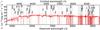 |
Fig. 5 Spectrum of a second example of a cluster galaxy (object 9). Lines and legends are the same as in Fig. 4. |
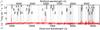 |
Fig. 6 Spectrum of object 5, one of the two cluster galaxies classified in this work as active, based on its (clearly visible) emission lines. Lines and legends are the same as in Fig. 4. |
3.2. Background galaxies
We identified many other sources that are not part of AS1063. Only two sources are found to have a redshift placing them in front of the cluster. These foreground galaxies are identified on a set of hydrogen emission lines (e.g. H α and H β).
3.2.1. Intermediate z galaxies
Properties of the detected background or foreground galaxies in the observed field.
We identified 17 galaxies behind the cluster. A total of 11 out of these 17 galaxies are intermediate redshift sources (0.4 <z< 1.5), and we clearly detect [O ii] λλ3726.0,3728.8 Å in emission for each of these 11 galaxies. When [O iii] λ4959.0 Å or [O iii] λ5006.8 Å fall inside the MUSE wavelength range (six galaxies), we also identified these emission lines. Only five out of these intermediate redshift galaxies show a continuum, while for the other six only emission lines are seen.
At intermediate and high redshifts, MUSE is well suited to study the kinematic profile of galaxies. To illustrate the power of MUSE at this, we created a velocity map for one of the intermediate redshift galaxies, object 38 in Table 2 at z = 0.607. This galaxy has a disk-like morphology and a clear continuum with strong emission lines. The large size of this galaxy, ~5′′ or ~33 kpc, and its edge-on orientation make it ideal to illustrate how MUSE can resolve the rotation pattern. We fit a Gaussian to the [O ii] emission line profile at every spatial location, and determine the velocity offset with respect to the central spaxels. We show the resulting velocity map in Fig. 7. The galaxy shows symmetrical rotation and the velocity reaches ~ 200 km s-1 at the largest radii. Velocity maps of other emission lines like [O iii] and H β show similar maps, but their analysis is hindered by the presence of skylines.
Sixteen lensed images, belonging to seven individual galaxies, that were found by Monna et al. (2014) are situated within our field. We identified ten out of these sixteen images, and determined their redshifts. Two triple-lensed galaxies are at intermediate redshifts, which we identified as sources 6 and 7 from Monna et al. (2014) and our sources 46 and 43, respectively, and four images correspond to galaxies at higher redshift, see Sect. 3.2.2. Galaxy 43 is at a redshift of z = 1.035, independently obtained from all detections 43a, 43b, and 43c. In addition, we detect source 46 at three different places, and we measured a redshift of z = 1.428 at each location. This is consistent with the redshift reported by Balestra et al. (2013, source 6a, z = 1.429, Richard et al. (2014a, source 2, z = 1.429, and Johnson et al. (2014).
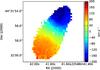 |
Fig. 7 [O ii] velocity map of galaxy 38 at z = 0.607. The coordinates are shown on the axes, and the velocity is given for every pixel by its colour. This figure clearly illustrates the power of MUSE for 2D spectroscopy. |
3.2.2. High-redshift galaxies
We identified one galaxy (source 48) in the redshift gap 1.5 <z< 2.9 where neither [O ii] or Lyαare redshifted into the MUSE wavelength range. The redshift measurement of z = 2.577 is based on C iii] λ 1907 Å, and secure thanks to a previous redshift determination with VIMOS (Balestra et al., in prep). A skyline prevents the detection of C iii] λ 1909 Å, and no other emission lines are found for this source.
At redshift z ~ 3, we found two other sources (49a&b) previously recognised by Monna et al. (2014) as a lensed galaxy (their sources 11a and 11b, see Fig. 2c for a zoom in with MUSE), and we measured a redshift of z = 3.116 for them. This redshift is consistent with the result found by Balestra et al. (2013) and Johnson et al. (2014), and we find additional emission lines at 6372.5, 6383.4, 6750, and 6857 Å. We identified these lines as C ivλλ1548,1550 Å, He iiλ1640, O iii] λ1666, and C iii] λ1907 Å, see Fig. 8. Clear detections of O iii] λ1661 and C iii] λ1909 Å are not seen in the datacube, because they are largely covered by a skyline. The redshift that we measured from all of these emission lines is within Δz< 0.001 of z = 3.116. The emission lines suggest AGN activity in this galaxy (e.g. Hainline et al. 2011), however, we do not detect any N v emission commonly seen in AGN. We compared the flux ratios to those found in the Lynx arc (Fosbury et al. 2003; Binette et al. 2003) and the M2031 arc at z = 3.51 (Christensen et al. 2012b). We assumed that the ratio of the C iii] and C iv doublets are equal, in order to estimate the flux of C iii] λ1909. The ratio of C iv/C iii] = 3.4, which is much higher than in the Lynx arc, suggesting AGN activity. The flux ratio of C iv/He ii = 5 is significantly lower than for a hot star cluster, supporting the ratio of C iv/C iii] as possible evidence of AGN activity.
By inspecting the profile of Lyαemission for this galaxy, we can derive some important properties. First, the profile is clearly double peaked and asymmetric. Second, the peak Lyαemission is at 1216.15 Å, see Fig. 9, resulting in a redshift of 100 km s-1 compared to the other UV-emission lines. This velocity difference is significantly smaller than observed in z = 2 − 3 Lyman break galaxies (~ 400 km s-1; e.g. Shapley et al. 2003; Steidel et al. 2010), but comparable to the differences found for z = 5.7Lyα emitters (LAEs; Diaz et al., in prep.) and LAEs in several other studies (e.g. Christensen et al. 2012a; Hashimoto et al. 2013; Shibuya et al. 2014). Third, we measure that the velocity difference between the red and the blue peak is Δv = 350 km s-1, half of what is found in star forming (Kulas et al. 2012) and massive galaxies (Karman et al. 2014) at z ~ 3. The center of the absorption trough is slightly blueshifted compared to the observed emission lines. Last, we see that the spatial profile of the Lyαpeaks is very homogeneous with a constant velocity over both sources and two clear elliptical shapes. However, this homogeneous shape is likely the result of the seeing during the observations.
We also identified three additional galaxies based on Lyαemission that were not reported before, and we show the stacked full-resolution 1D spectra of each of these galaxies in Fig. 9. The first galaxy, ID 51, lies at a short distance from source 49 at 5140 Å. The line has a clear asymmetry with a red tail and no other features at other wavelength are evident. Therefore, we determine the redshift to be z = 3.228.
The second source, ID 50, is a line emitter with an arc-like structure, see Fig. 2d. This emission line has a central wavelength of 5006.3 Å and no other emission is found for this source. Assigning Lyαto this emission results in a redshift z = 3.117. There is a clear red and blue peak in this source, and we measured a velocity difference of 500 km s-1 between the two peaks.
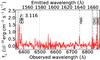 |
Fig. 8 MUSE 1D spectrum of source 49b, with wavelength on the horizontal axis and the flux on the vertical axis. The spectrum is zoomed in on the emission lines identified as C iv, He ii, and O iii]. Lines and legends are the same as in Fig. 4. |
The third new high redshift galaxy that we found is source 52. It is located slightly below the arc identified as 7a by Monna et al. (2014) and has two slightly elongated emission features at 6216.3 Å, see Fig. 2b. The profile of this emission line is asymmetric with a red wing, but we do not find a second peak, see Fig. 9. If this emission corresponded to a restframe optical nebular emission line, e.g. H α, other emission lines should be visible in our data. Because we do not find any other emission line and given the profile of the emission, we conclude that these emission lines must be Lyαand that both detections are very likely new multiply lensed images of the same galaxy at z = 4.113. The location of the images are consistent with submitted lens models for the Frontier Fields, and a fainter third image is predicted north-west of the field.
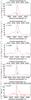 |
Fig. 9 Full-resolution MUSE 1D spectrum of sources (top to bottom) 49, 50, 51, 52, and 53, with wavelength on the horizontal axis and the flux on the vertical axis. The spectra are zoomed in on the Lyαline, which is indicated by the vertical black line. For source 49, we determined the redshift based on other UV-emission lines, while for the other sources we used Lyαto determine z. For sources 49, 52, and 53 the different images of the same source are stacked to optimise the signal-to-noise ratio. The fluctuations and non-zero continuum around Lyαin object 53 are the result of locally increased noise. |
The highest redshift source that we found is a galaxy at redshift z = 6.107. This galaxy is discussed in detail as a quintiply lensed galaxy by Balestra et al. (2013), Richard et al. (2014a), and Johnson et al. (2014). We identified both lensed images (53a&b) that were reported before in our field, and show the stacked Lyαprofile in Fig. 9. In Fig. 2a we have marked a tentative additional source that has the same redshift as the multiply lensed z = 6.107 galaxy. Although the signal at this location is weak, the source appears and disappears at identical wavelength (around 8641.3 Å) as the sources 53a&b. This additional image is not predicted by the lens models, and there is no clear detection in any of the HST images. If this is the same source, we can use the ratio of the Lyαline flux in different images to calculate the magnitude at different wavelengths. We find a flux ratio of 5−10, and when we compare the expected magnitudes to the limits in the HST images, we find that for the lower ratio the source should be visible in the F105W band, and for the higher ratio we expect a 2σ measurement. We caution that this is a tentative detection, and we call this galaxy 53c, but we emphasise that it still needs to be confirmed whether this is indeed another image of the multiply lensed source, or a companion galaxy.
The small difference in redshift that we and Richard et al. (2014a) find compared to Balestra et al. (2013), z = 6.107 versus z = 6.110, is likely due to a difference in spectral resolution and the proximity of a weak sky line. Contrary to Balestra et al. (2013) we do not detect any continuum in any of the images. Although the exposure time is comparable, the brightest image is close to the edge of our field, and this causes an increased noise level in our datacube. Therefore, the weak continuum that was observed previously, is lost to the locally increased noise in our observations.
4. Narrow-band images
We exploited the large wavelength range of MUSE to construct narrowband images of ~ 5 − 10 Å wide from 6000 Å to 9300 Å. We created these in order to look for emission lines or weak continuum detections corresponding to additional high redshift galaxies, which were not identified through visual inspection of the datacube. We placed the narrowbands around the atmospheric lines, excluding wavelengths with bright atmospheric emission, and determined their width to optimise the number of bands. Because the width of these bands is comparable to the width of Lyαemission lines, we expect that high redshift LAEs only show up in one to three bands.
We used the photometric catalogues created by the CLASH Image Pipeline to compile a list of additional high redshift candidates in our field. We ran Sextractor on the 193 MUSE narrow-band images, and found no detections that lie within 1′′ to the positions of these high redshift candidates. We found five new galaxies that occur in many of the redder images using this approach, that are not close to the location of any high-redshift candidate. Because they show continuum at longer wavelengths without detections at shorter wavelengths, it is likely that the 4000 Å or Lyman break is observed. The 4000 Å break only falls inside of the MUSE wavelength range at low redshift (z< 1.2), while the Lyman break is inside the MUSE wavelength range at high redshift (z> 4.2). Therefore, depending on which break is observed, these galaxies could be either at high or low redshift. We labelled these sources in Table 2 with IDs higher than 60.
5. Summary and conclusions
We presented VLT/MUSE observations of the cluster AS1063, and provided redshift measurements for 53 galaxies. We measured redshifts for 34 cluster galaxies, including 29 new determinations, and 17 galaxies at higher redshifts. Five of the detected galaxies show two or three lensed images in our field, and they are often seen on arcs.
We found that almost all cluster galaxies show spectra that are representative of old stellar populations, with a strong Balmer break and prominent Ca ii absorption lines. Only three out of the 34 show emission lines that indicate star formation activity.
At intermediate redshifts (0.4 <z< 1.5), we identified 11 galaxies. All of these galaxies show clear [O ii] emission lines and additional emission lines if they are within the MUSE wavelength range, but only two show a clear continuum. As [O ii] moves outside of the spectral range at a redshift of z> 1.5 and Lyαonly falls inside at redshifts z> 2.9, we do not find any galaxies in between these redshifts. Recently, Stark et al. (2014) argued that C iii] λ1909 Å is the best alternative in the UV to detect low-metallicity low-mass star-forming galaxies if Lyαis unavailable (see also Balestra et al. 2010). The spectral resolution of MUSE is sufficient to resolve the C iii] doublet, disentangling among different emission lines, even with single line detections, as demonstrated by Richard et al. (2014b). As C iii] falls inside the wavelength coverage of MUSE at redshifts 1.5 <z< 3.9, deeper observations can fill the currently observed redshift gap at 1.5 <z< 2.9 with C iii] emitters. We used a LAE at z = 2.577 (source 48, see Balestra et al., in prep.) to confirm this, and find an emission line at the wavelength corresponding to C iii] λ1907.
At z> 3 we detect five galaxies, of which three were not reported before. This includes the detection of a new multiply lensed galaxy at z = 4.113, with coordinates consistent with lens model predictions. We identified two of the images reported by Balestra et al. (2013) as a quintiply lensed galaxy at z = 6.107.
It is interesting to note that Boone et al. (2013) reported an excess of 870 μm emission in this cluster. While two heavily star-forming galaxies (objects 6 and 38) can explain the infrared emission from 3.6−500 μm, and most of the south-west 870 μm emission, they cannot explain the large 870 μm flux in the north-east. Boone et al. (2013) argued that this excess could be explained by either substructures in the Sunyaev-Zel’dovich effect, or a sub-mm galaxy at z> 4. In particular, they suggest that the multiply lensed z = 6.107 galaxy or a companion galaxy could be the optical counterpart to this excess.
In our field we found three possible counterparts to such z> 4 sub-mm galaxy. First, the quintiple-lensed z = 6.107 galaxy (sources 53a&b) was shown to have a very blue UV-slope by Balestra et al. (2013), which they argued is incompatible with the amount of dust needed for a sub-mm galaxy. The second possible counterpart is object 53c, as this could be a companion galaxy to the quintiply-lensed z = 6.107 galaxy. However, the lensing models do not predict any image of this source to the NE where most of the sub-mm excess is found. Therefore, we find it unlikely that this galaxy is a major contributor to the 870 μm flux. The last possible z> 4 contributor to this flux is the newly detected z = 4.113 double-lensed LAE. For this galaxy, the lens models do not predict an image at the NE either, making this source equally unlikely to be significantly contributing to the 870 μm flux. Therefore, we believe that it is unlikely that any of the galaxies discussed in this paper are the optical counterpart to the sub-mm source detected by Boone et al. (2013).
For one lensed Lyαemitting galaxy at z = 3.116, we find additional emission lines that correspond to C iv, He ii, O iii], and C iii], with flux ratios indicative of an AGN. We remark that although we favour the AGN interpretation, it is possible that these emission lines are coming from a cluster of hot O-stars. Ouchi et al. (2008) studied the AGN fraction as a function of Lyαluminosity for LAEs at z = 3 − 4. We determined the Lyαflux of this object, and compare to the results of Ouchi et al. (2008) to assess how common it is. We measured a Lyαflux of f = 1.4 × 10⁻¹⁶ erg s-1 cm-2, corresponding to an observed luminosity of L ≈ 5 × 1043 erg s-1 at this redshift. From the magnification maps distributed by the HST Frontier Fields programme, we obtained a magnification factor varying from 5 to 20, depending on the lensing model. This results in an intrinsic luminosity of L = 2.5 − 10 × 1043 erg s-1. Ouchi et al. (2008) found that at least 10 per cent of LAEs with similar Lyαluminosities host an AGN.
All of the high-z galaxies show a clearly asymmetric Lyαline profile, with a red wing which is more extended than the blue side, and two show a large red peak in combination with a smaller blue peak. The velocity difference between the two peaks is significantly smaller than seen in most previous studies. Christensen et al. (2012b) find a similar peak velocity difference in their lensed sources. A possible explanation is that by observing lensed sources, we find less massive galaxies with smaller gas-expansion speeds, and as a result a less blueshifted second peak. The Lyαemission lines all show a regular spatial elliptical shape, which are aligned with the detected arcs. As these shapes could be the result of the lensing and seeing conditions, we can unfortunately not draw any conclusions about the intrinsic shape. With the future implementation of Adaptive Optics at MUSE, these structures should become clearly resolved.
It is interesting to compare the photometric redshifts, as estimated by the CLASH team, with the MUSE spectroscopic redshifts. We show this comparison in Fig. 10. The agreement found for the background galaxies is very good, the cluster members instead show a larger degree of scatter.
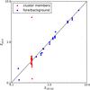 |
Fig. 10 Comparison of the photometric redshifts as calculated by the CLASH team based on HST multiband photometry, with the MUSE spectroscopic redshifts measured in this study. Red circles correspond to cluster members, while the blue squares correspond to foreground and background galaxies. Objects 43b and 51 are not deblended in the HST images, objects 19 and 53a are missing several bands, and object 53c has no HST detections, and are therefore all excluded from this plot. |
In this study, we show the breadth of science that a single MUSE pointing, with modest exposure time, is able to address. At high-z, it allows for the detection and characterisation of galaxies through Lyαdetection, rest-frame UV lines, and morphology. At low and intermediate redshifts, it enables the construction of rotation maps, the study of internal dynamics, the determination of the ionisation source in the galaxy through emission line ratios, and accurate stellar population studies. At low redshifts, the properties will be obtained in high detail, and in addition, star formation rates can be determined from H α.
This Article shows the strength of using MUSE in both blind and targeted searches for high-redshift galaxies in magnifying clusters. The additional advantage of MUSE, when observing magnifying clusters, is that one simultaneously observes the whole Einstein volume of the cluster in one pointing. MUSE provides both a high spatial and spectral resolution, has a large FOV and spectral range. These properties make it ideal to study line profiles and look for additional features without the problem of source confusion. As the performance is good over long times, it is well suited for long exposures in empty sky fields. MUSE will therefore provide a very large number of galaxies with redshift identifications up to a redshift of z< 6.6, and is expected to significantly increase our understanding of the formation and evolution of galaxies at z> 3.
Acknowledgments
Based on observations made with the European Southern Observatory Very Large Telescope (ESO/VLT) at Cerro Paranal, under programme ID 60.A-9345(A). This work utilises gravitational lensing models produced by PIs Bradać, Ebeling, Merten & Zitrin, Sharon, and Williams funded as part of the HST Frontier Fields programme conducted by STScI. STScI is operated by the Association of Universities for Research in Astronomy, Inc. under NASA contract NAS 5-26555. The lens models were obtained from the Mikulski Archive for Space Telescopes (MAST). The authors thank the anonymous referee for his/her helpful comments that improved the clarity of this article. The authors also thank Thomas Martinsson for help with the MUSE pipeline, Benjamin Clement for support in designing the observations, and Elena Valenti and Vicenzo Mainieri for technical support during the observation planning and data reduction phase. The Dark Cosmology Centre is funded by the DNRF.
References
- Bacon, R., Accardo, M., Adjali, L., et al. 2010, in SPIE Conf. Ser., 7735 [Google Scholar]
- Bacon, R., Accardo, M., Adjali, L., et al. 2012, The Messenger, 147, 4 [NASA ADS] [Google Scholar]
- Balestra, I., Mainieri, V., Popesso, P., et al. 2010, A&A, 512, A12 [NASA ADS] [CrossRef] [EDP Sciences] [Google Scholar]
- Balestra, I., Vanzella, E., Rosati, P., et al. 2013, A&A, 559, L9 [NASA ADS] [CrossRef] [EDP Sciences] [Google Scholar]
- Bertin, E., & Arnouts, S. 1996, A&AS, 117, 393 [NASA ADS] [CrossRef] [EDP Sciences] [Google Scholar]
- Binette, L., Groves, B., Villar-Martín, M., Fosbury, R. A. E., & Axon, D. J. 2003, A&A, 405, 975 [NASA ADS] [CrossRef] [EDP Sciences] [Google Scholar]
- Biviano, A., Rosati, P., Balestra, I., et al. 2013, A&A, 558, A1 [NASA ADS] [CrossRef] [EDP Sciences] [Google Scholar]
- Blanc, G. A., Adams, J. J., Gebhardt, K., et al. 2011, ApJ, 736, 31 [NASA ADS] [CrossRef] [Google Scholar]
- Böhringer, H., Schuecker, P., Guzzo, L., et al. 2004, A&A, 425, 367 [NASA ADS] [CrossRef] [EDP Sciences] [Google Scholar]
- Boone, F., Clément, B., Richard, J., et al. 2013, A&A, 559, L1 [NASA ADS] [CrossRef] [EDP Sciences] [Google Scholar]
- Christensen, L., Laursen, P., Richard, J., et al. 2012a, MNRAS, 427, 1973 [NASA ADS] [CrossRef] [Google Scholar]
- Christensen, L., Richard, J., Hjorth, J., et al. 2012b, MNRAS, 427, 1953 [Google Scholar]
- Coe, D., Umetsu, K., Zitrin, A., et al. 2012, ApJ, 757, 22 [NASA ADS] [CrossRef] [Google Scholar]
- Contini, T., Garilli, B., Le Fèvre, O., et al. 2012, A&A, 539, A91 [NASA ADS] [CrossRef] [EDP Sciences] [Google Scholar]
- Curtis-Lake, E., McLure, R. J., Pearce, H. J., et al. 2012, MNRAS, 422, 1425 [NASA ADS] [CrossRef] [EDP Sciences] [Google Scholar]
- Epinat, B., Contini, T., Le Fèvre, O., et al. 2009, A&A, 504, 789 [NASA ADS] [CrossRef] [EDP Sciences] [Google Scholar]
- Erb, D. K., Shapley, A. E., Pettini, M., et al. 2006a, ApJ, 644, 813 [NASA ADS] [CrossRef] [Google Scholar]
- Erb, D. K., Steidel, C. C., Shapley, A. E., et al. 2006b, ApJ, 646, 107 [NASA ADS] [CrossRef] [Google Scholar]
- Finkelstein, S. L., Papovich, C., Dickinson, M., et al. 2013, Nature, 502, 524 [NASA ADS] [CrossRef] [Google Scholar]
- Förster Schreiber, N. M., Genzel, R., Lehnert, M. D., et al. 2006, ApJ, 645, 1062 [NASA ADS] [CrossRef] [Google Scholar]
- Fosbury, R. A. E., Villar-Martín, M., Humphrey, A., et al. 2003, ApJ, 596, 797 [NASA ADS] [CrossRef] [Google Scholar]
- Fumagalli, M., Fossati, M., Hau, G. K. T., et al. 2014, MNRAS, submitted [arXiv:1407.7527] [Google Scholar]
- Gómez, P. L., Valkonen, L. E., Romer, A. K., et al. 2012, AJ, 144, 79 [NASA ADS] [CrossRef] [Google Scholar]
- Grillo, C., Gobat, R., Presotto, V., et al. 2014a, ApJ, 786, 11 [NASA ADS] [CrossRef] [Google Scholar]
- Grillo, C., Suyu, S. H., Rosati, P., et al. 2014b, ApJ, submitted [arXiv:1407.7866] [Google Scholar]
- Guaita, L., Francke, H., Gawiser, E., et al. 2013, A&A, 551, A93 [NASA ADS] [CrossRef] [EDP Sciences] [Google Scholar]
- Guzzo, L., Schuecker, P., Böhringer, H., et al. 2009, A&A, 499, 357 [NASA ADS] [CrossRef] [EDP Sciences] [Google Scholar]
- Hainline, K. N., Shapley, A. E., Greene, J. E., & Steidel, C. C. 2011, ApJ, 733, 31 [NASA ADS] [CrossRef] [Google Scholar]
- Hashimoto, T., Ouchi, M., Shimasaku, K., et al. 2013, ApJ, 765, 70 [NASA ADS] [CrossRef] [Google Scholar]
- Johnson, T. L., Sharon, K., Bayliss, M. B., et al. 2014, ApJ, submitted [arXiv:1405.0222] [Google Scholar]
- Jouvel, S., Host, O., Lahav, O., et al. 2014, A&A, 562, A86 [NASA ADS] [CrossRef] [EDP Sciences] [Google Scholar]
- Kajisawa, M., Ichikawa, T., Yamada, T., et al. 2010, ApJ, 723, 129 [NASA ADS] [CrossRef] [Google Scholar]
- Karman, W., Caputi, K. I., Trager, S. C., Almaini, O., & Cirasuolo, M. 2014, A&A, 565, A5 [NASA ADS] [CrossRef] [EDP Sciences] [Google Scholar]
- Kulas, K. R., Shapley, A. E., Kollmeier, J. A., et al. 2012, ApJ, 745, 33 [NASA ADS] [CrossRef] [Google Scholar]
- Le Fèvre, O., Cassata, P., Cucciati, O., et al. 2013, A&A, 559, A14 [NASA ADS] [CrossRef] [EDP Sciences] [Google Scholar]
- Maier, C., Lilly, S. J., Ziegler, B., et al. 2014, ApJ, 792, 3 [NASA ADS] [CrossRef] [Google Scholar]
- Mannucci, F., Cresci, G., Maiolino, R., et al. 2009, MNRAS, 398, 1915 [NASA ADS] [CrossRef] [Google Scholar]
- Monna, A., Seitz, S., Greisel, N., et al. 2014, MNRAS, 438, 1417 [NASA ADS] [CrossRef] [Google Scholar]
- Ouchi, M., Shimasaku, K., Akiyama, M., et al. 2008, ApJS, 176, 301 [NASA ADS] [CrossRef] [Google Scholar]
- Pentericci, L., Fontana, A., Vanzella, E., et al. 2011, ApJ, 743, 132 [NASA ADS] [CrossRef] [Google Scholar]
- Postman, M., Coe, D., Benítez, N., et al. 2012, ApJS, 199, 25 [NASA ADS] [CrossRef] [Google Scholar]
- Richard, J., Jauzac, M., Limousin, M., et al. 2014a, MNRAS, 444, 268 [NASA ADS] [CrossRef] [Google Scholar]
- Richard, J., Patricio, V., Martinez, J., et al. 2014b, MNRAS, submitted [arXiv:1409.2488] [Google Scholar]
- Shapley, A. E., Steidel, C. C., Pettini, M., & Adelberger, K. L. 2003, ApJ, 588, 65 [NASA ADS] [CrossRef] [Google Scholar]
- Shibuya, T., Kashikawa, N., Ota, K., et al. 2012, ApJ, 752, 114 [Google Scholar]
- Shibuya, T., Ouchi, M., Nakajima, K., et al. 2014, ApJ, 788, 74 [NASA ADS] [CrossRef] [Google Scholar]
- Stark, D. P., Ellis, R. S., & Ouchi, M. 2011, ApJ, 728, L2 [NASA ADS] [CrossRef] [Google Scholar]
- Stark, D. P., Richard, J., Siana, B., et al. 2014, MNRAS, submitted [arXiv:1408.1420] [Google Scholar]
- Steidel, C. C., Erb, D. K., Shapley, A. E., et al. 2010, ApJ, 717, 289 [NASA ADS] [CrossRef] [Google Scholar]
- Talia, M., Mignoli, M., Cimatti, A., et al. 2012, A&A, 539, A61 [NASA ADS] [CrossRef] [EDP Sciences] [Google Scholar]
- van Dokkum, P. G. 2001, PASP, 113, 1420 [NASA ADS] [CrossRef] [Google Scholar]
- Vanzella, E., Fontana, A., Zitrin, A., et al. 2014, ApJ, 783, L12 [NASA ADS] [CrossRef] [Google Scholar]
- Zitrin, A., Meneghetti, M., Umetsu, K., et al. 2013, ApJ, 762, L30 [NASA ADS] [CrossRef] [Google Scholar]
All Tables
Properties of the detected background or foreground galaxies in the observed field.
All Figures
|
Fig. 1 Red-green-blue image composition of HST images of the part of AS1063 that we observed with MUSE, where the colours in this image are blue = F435W + F475W, green = F606W + F625W + F775W + F814W + F850LP, red = F105W + F110W + F140W + F160W. The individual HST images were obtained and distributed by the CLASH collaboration. The green square delimits the 1 × 1′ MUSE FOV. All 19 objects with a spectroscopic redshift z> 1 are shown as white circles and their redshifts. Numbered galaxies were noted before by Monna et al. (2014) and Balestra et al. (2013). The blue, magenta, and red contours correspond to regions where the magnification is μ> 200 at z = 1, 2, and 4, respectively. The magnifications are based on the second version of the Sharon models (Johnson et al. 2014), which were chosen for illustrative purposes, but we note that this is only one out of many different available models. |
| In the text | |
|
Fig. 2 Snapshot of our MUSE pointing towards Abell S1063. Left: a slice of reduced MUSE data cube centred at 7250 Å with Δλ = 1.25 Å. Right: zoom-ins of the four regions with LAEs marked on the left panel, where the wavelength is centred at the peak of Lyαfor galaxies 53a,c 52a,b, 49a,b, and 50 in panels A, B, C, and D, respectively. In zoom-in A, we placed a circle around the weak additional detection of the quintiply lensed galaxy at z = 6.107. |
| In the text | |
|
Fig. 3 Distribution map of the identified cluster galaxies. Squares correspond to passive galaxies, while stars indicate active galaxies, where their classification is based on the presence or absence of optical emission lines. The galaxies have been coloured according to their velocity relative to the cluster, with bluer colours meaning higher velocities towards us, and redder colours corresponding to higher velocities away from us. |
| In the text | |
|
Fig. 4 Spectrum of a typical cluster galaxy (object 2). The red line represents the 1D spectrum, where the source is extracted as an ellipse with typically 1″ × 1″ axes and then summed in the spatial direction. The grey line represents the level of dispersion in the global sky, while the black dashed vertical lines represent restframe wavelengths of the most important transitions. At skylines grey vertical lines are plotted, and the redshift is shown in the top right corner. |
| In the text | |
|
Fig. 5 Spectrum of a second example of a cluster galaxy (object 9). Lines and legends are the same as in Fig. 4. |
| In the text | |
|
Fig. 6 Spectrum of object 5, one of the two cluster galaxies classified in this work as active, based on its (clearly visible) emission lines. Lines and legends are the same as in Fig. 4. |
| In the text | |
|
Fig. 7 [O ii] velocity map of galaxy 38 at z = 0.607. The coordinates are shown on the axes, and the velocity is given for every pixel by its colour. This figure clearly illustrates the power of MUSE for 2D spectroscopy. |
| In the text | |
|
Fig. 8 MUSE 1D spectrum of source 49b, with wavelength on the horizontal axis and the flux on the vertical axis. The spectrum is zoomed in on the emission lines identified as C iv, He ii, and O iii]. Lines and legends are the same as in Fig. 4. |
| In the text | |
|
Fig. 9 Full-resolution MUSE 1D spectrum of sources (top to bottom) 49, 50, 51, 52, and 53, with wavelength on the horizontal axis and the flux on the vertical axis. The spectra are zoomed in on the Lyαline, which is indicated by the vertical black line. For source 49, we determined the redshift based on other UV-emission lines, while for the other sources we used Lyαto determine z. For sources 49, 52, and 53 the different images of the same source are stacked to optimise the signal-to-noise ratio. The fluctuations and non-zero continuum around Lyαin object 53 are the result of locally increased noise. |
| In the text | |
|
Fig. 10 Comparison of the photometric redshifts as calculated by the CLASH team based on HST multiband photometry, with the MUSE spectroscopic redshifts measured in this study. Red circles correspond to cluster members, while the blue squares correspond to foreground and background galaxies. Objects 43b and 51 are not deblended in the HST images, objects 19 and 53a are missing several bands, and object 53c has no HST detections, and are therefore all excluded from this plot. |
| In the text | |
Current usage metrics show cumulative count of Article Views (full-text article views including HTML views, PDF and ePub downloads, according to the available data) and Abstracts Views on Vision4Press platform.
Data correspond to usage on the plateform after 2015. The current usage metrics is available 48-96 hours after online publication and is updated daily on week days.
Initial download of the metrics may take a while.