| Issue |
A&A
Volume 574, February 2015
|
|
|---|---|---|
| Article Number | A37 | |
| Number of page(s) | 12 | |
| Section | The Sun | |
| DOI | https://doi.org/10.1051/0004-6361/201323206 | |
| Published online | 21 January 2015 | |
Can we explain atypical solar flares?⋆
1
LESIA, Observatoire de Paris, LESIA, CNRS, UMPC, Univ. Paris Diderot,
5 place Jules
Janseen,
92190
Meudon,
France
e-mail:
This email address is being protected from spambots. You need JavaScript enabled to view it.
2
Department of Physics, DSB Campus, Kumaun
University, Nainital-
263 002,
India
Received: 6 December 2013
Accepted: 12 November 2014
Abstract
Context. We used multiwavelength high-resolution data from ARIES, THEMIS, and SDO instruments to analyze a non-standard, C3.3 class flare produced within the active region NOAA 11589 on 2012 October 16. Magnetic flux emergence and cancellation were continuously detected within the active region, the latter leading to the formation of two filaments.
Aims. Our aim is to identify the origins of the flare taking the complex dynamics of its close surroundings into account.
Methods. We analyzed the magnetic topology of the active region using a linear force-free field extrapolation to derive its 3D magnetic configuration and the location of quasi-separatrix layers (QSLs), which are preferred sites for flaring activity. Because the active region’s magnetic field was nonlinear force-free, we completed a parametric study using different linear force-free field extrapolations to demonstrate the robustness of the derived QSLs.
Results. The topological analysis shows that the active region presented a complex magnetic configuration comprising several QSLs. The considered data set suggests that an emerging flux episode played a key role in triggering the flare. The emerging flux probably activated the complex system of QSLs, leading to multiple coronal magnetic reconnections within the QSLs. This scenario accounts for the observed signatures: the two extended flare ribbons developed at locations matched by the photospheric footprints of the QSLs and were accompanied with flare loops that formed above the two filaments, which played no important role in the flare dynamics.
Conclusions. This is a typical example of a complex flare that can a priori show standard flare signatures that are nevertheless impossible to interpret with any standard model of eruptive or confined flare. We find that a topological analysis, however, permitted us to unveil the development of such complex sets of flare signatures.
Key words: Sun: flares / Sun: corona / Sun: filaments, prominences / Sun: magnetic fields / magnetic reconnection
Movies associated to Figs. 1, 3, and 9 are only available at the CDS via anonymous ftp to cdsarc.u-strasbg.fr (130.79.128.5) or via http://cdsarc.u-strasbg.fr/viz-bin/qcat?J/A+A/574/A37
© ESO, 2015
1. Introduction
Solar flares are the most energetic events on the Sun. They emit radiation over the whole electromagnetic spectrum from γ-rays to radio wavelengths (Shibata 1999; Shibata & Magara 2011). Magnetic reconnection is the main process that releases energy during the solar flares. This energy is extracted from the magnetic energy that is stored in current-carrying fields in the corona. During a flare, energetic particles and thermal energy are produced around the reconnection site. They flow down toward the lower and denser layers of the solar atmosphere. As a result, coronal emission is produced within and around (post) flare loops, and surface brightenings occur along so-called flare ribbons, as observed in the ultraviolet (UV), as well as in typically-chromospheric wavelengths such as Hα. Solar flares are usually classified into two categories: eruptive or confined.
When a flare is associated with a coronal mass ejection (CMEs), whether or not it is associated with a detectable filament eruption, it is an eruptive flare. Those are often referred to as two-ribbon flares and long duration events, because they are associated with two parallel flare ribbons that are located on both sides of the polarity inversion line (PIL) and that gradually move apart from one another. To explain the different observational manifestations of eruptive flares, such as filament eruptions when they are observed, ribbon separations, flare loops formation, and associated phenomena, the standard CSHKP flare model was developed in two dimensions (Carmichael 1964; Sturrock 1966; Hirayama 1974; Kopp & Pneuman 1976; Forbes & Malherbe 1986). According to this model, a current sheet forms in the corona, right below the erupting filament. Magnetic field lines sequentially reconnect at this current sheet, resulting in a growing (resp. spreading) system of flare loops (resp. ribbons), located below the erupting filament. Some 3D extensions to this model have been recently proposed to explain observational properties and physical processes, first in the form of cartoons (Shibata et al. 1995; Moore et al. 2001; Priest & Forbes 2002) and, more recently, based on numerical simulations (Aulanier et al. 2012; Kusano et al. 2012; Janvier et al. 2013).
The other flares, which are not associated with a CME, are the confined flares. Those are classically due to loop-loop interactions in the corona, which are induced by horizontal motions or flux emergence through the photosphere (e.g., Gorbachev & Somov 1989; Démoulin et al. 1997; Hanaoka 1997; Mandrini et al. 1997; Schmieder et al. 1997; Nishio et al. 1997; Chandra et al. 2006). Confined flares are usually associated with multiple ribbons. The classical 2D picture for the magnetic configuration and reconnection behavior in such flares is that of a coronal X-point, where a current sheet is gradually formed as a result of the photospheric motions (Giovanelli 1947; Heyvaerts et al. 1977; Syrovatskii 1981; Low & Wolfson 1988; Aly & Amari 1997). Magnetic topology analyses of active regions have played a crucial role in understanding the magnetic reconnection processes in 3D in confined flares (see review by Démoulin 2007). In 2D configuration, the reconnection can occur at null points, where the magnetic field vanishes. In 3D, the reconnection can also occur at a null point (Masson et al. 2009), but also along a separator (e.g., Longcope 2005; Parnell et al. 2010a) or a quasi-separatrix layer (QSL, see, e.g., Démoulin et al. 1997; Titov et al. 2002; Aulanier et al. 2005; Pariat & Démoulin 2012).
Some atypical flares share several elements common to both the classical definition of eruptive and confined categories, in particular the existence of two parallel ribbons and several other remote ribbons. To the authors’ knowledge, three different origins are known for these complex events that, depending on each case, belong to either the eruptive or confined flares categories. Firstly, they can be due to a failed filament eruption. The confinement of the filament by coronal arcades makes it stall in the low corona and eventually reconnect with its restraining arcades (e.g., Török & Kliem 2005; Guo et al. 2010; Chen et al. 2013). Secondly, they can develop when long-distance loop-loop interactions and reconnections are driven by a successful eruption that pushes these loops against their neighbors (e.g., Maia et al. 2003; Chandra et al. 2009). Thirdly, they can appear when two filaments of opposite helicities reconnect with one another without merging (Deng et al. 2002; Schmieder et al. 2004; DeVore et al. 2005; Török et al. 2011; Chandra et al. 2011).
Because of their complexity, many atypical flares have not been analyzed in great detail. One could wonder if the usual tools and models that have been developed throughout the years are really relevant for all of these complex events. The question is more preoccupying than it sounds at first since these complex less-studied flares may be the most numerous of all the flares that the Sun produces. We note that the recent paper by Liu et al. (2014) was the first topological study that started addressing this question. Combining a careful EUV analysis with the QSL method, the authors were able to identify their event as being a confined flare associated with a failed flux rope eruption. The aim of our paper is to present and analyze a different but complex event that involved filaments, therefore using the standard flare model and the QSL method. Our single event was simply selected because it was observed with two independent ground based telescopes, namely THEMIS in Tenerife and ARIES in India. It was a C3.3 class flare, which occurred on 2012 Oct. 16 in the active region NOAA 11589. This region comprised two filaments that gradually formed and converged, but did not merge.
The QSL method was first proposed in Démoulin et al. (1997). It is based on the calculation of the photospheric footprints of QSLs from extrapolated magnetic fields. QSLs are defined as the narrow volumes within which the magnetic field connectivity has very sharp gradients (Priest & Démoulin 1995). They are the 3D generalization of separatrices in 2.5D X-points with an additional guide field (called flipping layers by Priest & Forbes 1992). QSLs are preferred sites for the build-up of electric currents and the development of magnetic reconnection in general 3D systems. Among many developments, QSLs have been shown to play an essential role not only in confined flares, but also in eruptive flares (Démoulin et al. 1996; Savcheva et al. 2012; Janvier et al. 2013), and possibly in SEP transport toward Earth (Masson et al. 2012), as well as in twisted flux tubes interacting in solar observations (Chandra et al. 2011), in numerical simulations (Milano et al. 1999; Wilmot-Smith et al. 2010; Török et al. 2011), and in laboratory experiments (Lawrence & Gekelman 2009; Gekelman et al. 2012). More details can be found in the reviews by Démoulin (2006) and Aulanier (2011). To conduct the QSL method (i.e., to plot the photospheric footprints of QSLs), either the norm N of the QSL (Démoulin et al. 1997) or its squashing degree Q (Titov et al. 2002) have to be calculated at the boundary of the extrapolated fields. Since both N and Q provide a different measure for the gradients of the field line connectivity across QSLs, their footprints naturally arise as narrow and elongated layers where N or Q ≫ 1. In this paper, we apply the QSL method to NOAA 11589 by computing the squashing degree, Q, at the photospheric level.
The paper is organized as follows. Section 2 presents the observations, with an analysis of the evolution of two filaments in the active region, and the development of the flare. The QSL method and the potential role of QSLs in the flare are discussed in Sect. 3. In Sect. 4, we present our interpretation of our results, with observational evidence of the trigger of the flare, and with a conjecture about the sequences of reconnections in the calculated QSLs that can account for the complex development of the observed atypical flare. Finally, in Sect. 5, we conclude on the important role of the QSL method in unveiling the sequence of events that shape complex and atypical flares, even when they do not fit the standard model.
2. Observations
2.1. Data
Part of the observations of NOAA 11589 presented here were obtained with the Atmospheric Imaging Assembly imager (AIA; Lemen et al. 2012) and the Helioseismic and Magnetic Imager (HMI; Schou et al. 2012) onboard the Solar Dynamic Observatory (SDO; Pesnell et al. 2012) satellite. The AIA instrument observes the Sun over a wide range of temperatures from the photosphere to the corona. The pixel size of the AIA images is 0.6′′. In this study, we considered the 1600, 304, 193, and 171 Å data. The magnetic field in the AR was studied by using the line-of-sight magnetograms of the HMI instrument, which observes the full disk with a pixel size of 0.5′′.
We also used ground-based observations of the AR obtained with the Indian telescope from the Aryabhatta Research Institute of observational Sciences (ARIES) and with the French Télescope Héliographique pour l’Etude du Magnétisme et des Instabilités Solaires (THEMIS). The 15-cm f/15 Coudé telescope of the ARIES, operating in Nainital (India), observes in the Hα line with a spatial resolution of 0.58′′. The THEMIS telescope, operating in Tenerife (Canary Islands), allows a simultaneous mapping of the Hα emission and the full Stokes parameters in the Fe 6302.5 Å of a field of view of about 240′′ × 100′′ in one hour.
2.2. Evolution of the photospheric magnetic field
The AR NOAA 11589 appeared at the heliographic coordinates N13 E61 on 2012 October 10. The AR appeared as two large-scale, decaying magnetic polarities. It presented a β magnetic configuration that evolved toward a βγδ configuration on October 16. During its on-disk passage, the AR produced 20 C-class flares.
The evolution of the AR during its on-disk passage presented localized magnetic flux emergence episodes together with large-scale magnetic flux cancellation as displayed in Fig. 1 (top row). The episodic emerging flux events occurred within the north of the central part of the AR. Figure 1 highlights two of these emerging flux events which occurred on October 13 and 14.
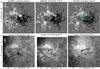 |
Fig. 1 Evolution of active region NOAA 11589 during its disk passage before the eruption on 2012 October 16. Top: evolution of the longitudinal magnetic field observed by SDO/HMI. White/black are positive/negative polarities. The field strength is saturated at 500 Gauss. The violet arrows indicate significant emerging fluxes on October 13 and 15. The cyan rectangle highlights the region where recurring magnetic flux emergence occurred on October 16 and likely triggered the studied C3-class flare (see Sect. 2.4). The temporal evolution of the magnetograms is available as a movie in the online edition. Bottom: development of filaments in Hα observed by ARIES telescope. The locations of two observed filaments F1 and F2 are indicated by black arrows. The white arrow indicates the north direction. |
The magnetogram evolution also presents traces of large-scale magnetic flux cancellation. In particular, we can see that the positive polarity that emerged on October 13, was progressively cancelled out. On October 16, this positive polarity had almost vanished. The large-scale flux cancellation is also observable in the central part of the AR, in the east part of the negative polarity. Indeed, it shows that the easternmost part of the negative polarity moved toward the east and progressively cancelled out with the positive polarity.
2.3. Evolution of the two active region filaments
The large-scale magnetic flux cancellation observed in the central part of the AR led to the formation of two filaments (e.g., van Ballegooijen & Martens 1989; Antiochos et al. 1994; Martens & Zwaan 2001; Wang & Muglach 2007). The evolution of these filaments in Hα is presented in Fig. 1 (bottom row). The formation of the first filament started on October 13 (see Fig. 1). The filament appeared in the southern part of the AR and progressively evolved toward the thick and elongated filament labeled F1 in the Hα image of Fig. 1. The second filament appeared on October 14 in the center of the AR and progressively evolved toward the filament labeled F2.
Using the Hα data from THEMIS (Fig. 2), we were able to derive the chirality of the filaments based on Aulanier & Démoulin (1998) and Mackay et al. (2010). In Fig. 2, one of the barbs of filament F1 indicates that the filament was dextral. In addition, the filament F1 had its easternmost end rooted in the positive polarity and its westernmost end rooted in the negative polarity. This indicates that its axial field was pointing towards the southwest. Regarding the position of the positive polarity compared with the negative polarity in this region (Fig. 1), it follows that the filament was dextral and thus had a negative helicity, which agrees with the orientation of the filament barbs. We note that the filament F1 thus obeyed the hemispheric chirality rule, according to which most of the filaments of the northern hemisphere have a dextral chirality (e.g., Pevtsov et al. 2003). Based on the same analysis, we found that the chirality of filament F2 was sinistral. The filament F2 thus had a positive helicity. It follows that F2 did not obey the hemispheric chirality rule. We thus conclude that NOAA 11589 possessed a mixed magnetic helicity, with positive magnetic helicity in its northern part and negative magnetic helicity in its southern part (see also Sect. 3.1).
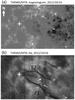 |
Fig. 2 Active region NOAA 11589 observed on 2012 October 16 by THEMIS/MTR between 08:02 and 09:02 UT. Top: longitudinal magnetic field. Bottom: Hα map showing the two recently formed filaments of Fig. 1. The white arrows indicate the barbs used to infer the filaments’ chirality. Filament F1 is a dextral filament and F2 is a sinistral filament. The + and − signs indicate the magnetic field polarity of each end of the filaments. The field of view covers ~ 175′′ × 100′′. The white arrow indicates the north direction. |
The evolution of these two filaments shows that the northern footpoints of both filaments converged toward each other without merging. This agrees with previous numerical simulation (e.g., DeVore et al. 2005; Aulanier et al. 2006a) and observational studies (e.g., Martin 1998; Schmieder et al. 2004; Chandra et al. 2010, 2011; Török et al. 2011) that show that the merging of two filaments strongly depends on their chirality and their relative orientation. In particular, the presented filaments evolution would be equivalent to Experiment 2 of DeVore et al. (2005, see their Fig. 8). Thus, the filaments did not have the opportunity of merging probably because their axial field was oriented in opposite directions along the PIL.
2.4. The 2012 October 16 flare
On 2012 October 16, the AR was located at heliographic coordinates N13 W11. On that day, the AR produced a C3.3/1F class flare. According to the GOES instruments, the flare started around 16:12 UT, peaked at 16:27 UT, and ended around 16:39 UT. The flare signatures were visible in the different wavelengths observed by the SDO. The 94 Å data from the SDO/AIA indicate that the flare was initiated in the northern part of the AR where magnetic flux emergence was often detected (Fig. 1).
 |
Fig. 3 Flare signatures observed by SDO/AIA on 2012 October 16 at 1600 Å (left), at 304 Å (middle), and at 171 Å (right). The black arrow indicates the northern direction. The white square indicates the field of view of Fig. 4. The temporal evolution of AIA 1600 Å, 304 Å, and 171 Å images is available as a movie in the online edition. |
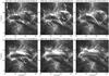 |
Fig. 4 Flare signatures observed by SDO/AIA on 2012 October 16 at 193 Å. In the top left panel, the white arrow indicates the northern direction. |
Figure 3 displays the flare signatures at 1600 and 304 Å during the maximum phase of the flare. These signatures present a similar morphology in both wavelengths. During the flare evolution, the data show the beginning of small, localized brightenings appearing on the northern, eastern, and southern parts of the AR. The eastern brightening, which was also the most distinguishable, progressively enhanced and expanded in the western direction. It formed within the positive polarity, and eventually developed into the eastern ribbon of Fig. 3. The northern brightening, which was the least distinguishable, expanded in both the eastern and western directions. It developed into the northern ribbon of Fig. 3 that formed within the positive polarity. This northern ribbon expanded and eventually merged with the eastern ribbon, forming a single, extended ribbon within the positive polarity of the AR. The southern brightening, which formed within the negative polarity, expanded in the northwest direction, forming the extended southern ribbon. Overall, the observations show that the flare ribbons developed into two single, extended ribbons that formed around both filaments, one ribbon within the positive polarity, the other within the negative polarity. We note that such ribbons are compatible with the two typical flare ribbons associated with the classical eruptive and confined flares involving the presence of a filament. Finally, the observations indicate that, at the extended southern ribbon, another brightening developed toward the southwest between 16:14 and 16:39 UT. This brightening was probably related to plasma ejection.
Figure 4 presents the evolution of the flare signatures during the decay phase at 193 Å. In this figure, we clearly see the formation of post-flare loops joining the two extended flare ribbons displayed in Fig. 3. From the AR evolution at 193 and 171 Å, we find that the first post-flare loops developed in the northern part of the AR. One of these northern post-flare loops is labeled L1 in Fig. 4. This post-flare loop was quickly followed by the formation of post-flare loops L2 and L3 within the central part of the AR. These post-flare loops were then followed by the formation of L4, and a bulk of post-flare loops in the central part of the AR.
According to the CSHKP model, both eruptive and confined flares – involving the presence of a filament – should be associated with the formation of hot post-flare loops below the erupting filament, regardless of whether its eruption succeeds or fails (see also Schmieder et al. 1995, 1996; Shibata & Magara 2011; Aulanier et al. 2012). Interestingly, we find that the post-flare loops formed above the filaments. Furthermore, the observations indicate that none of the two filaments seemed to be neither disturbed nor erupting during or after the flare. These two features are not consistent with any standard model of eruptive or confined flare. It follows that the two extended flare ribbons associated with the flare can be explained neither by a successful nor a failed filament eruption. A topological analysis is then required to build up a plausible flare scenario that explains the observed flare dynamics and its associated signatures.
3. Magnetic topology of the active region
3.1. Magnetic field extrapolation
The topological analysis of the AR 11589 magnetic field requires knowledge of the magnetic field in the coronal volume containing the AR. In practice, the coronal magnetic field can be estimated from linear (e.g., Nakagawa & Raadu 1972; Alissandrakis 1981; Démoulin et al. 1989) or nonlinear (see reviews by Wiegelmann & Sakurai 2012; Régnier 2013, and references therein) force-free field extrapolations (LFFF or NLFFF), defined by 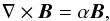 (1)using photospheric data as a bottom boundary condition. In Eq. (1), the force-free parameter, α, is uniform in space for LFFF extrapolations and is constant along each elemental flux tubes for NLFFF extrapolations.
Recent studies have shown that NLFFF extrapolations are becoming more and more reliable for inferring the coronal magnetic field from photospheric vector magnetograms (e.g., Schrijver et al. 2008; Canou & Amari 2010; Valori et al. 2012; Wiegelmann et al. 2012; Guo et al. 2012; Jiang & Feng 2013). Because the EUV data show that AR 11589 was formed of filaments of opposite chirality (see Fig. 2) and loops of opposite α values (see Eq. (1)), one may want to consider NLFFF extrapolations to study the topology of the AR.
However, there are two reasons for not considering such extrapolation models in the present study. First, the filaments were located in the plage regions, hence where the magnetic field is weak and the photospheric electric currents, and local α-values, are not well measured. This would tend to give a nearly potential magnetic field within these regions, which would prevent retrieving the filaments in an NLFFF extrapolation (e.g., McClymont et al. 1997; Leka & Skumanich 1999; Wiegelmann 2004). The second reason is given by the EUV data showing that none of the filaments seemed to be affected by the evolution of the flare. Indeed, both filaments were still present with the same shape before and after the flare. In addition, the EUV data show that the post-flare loops were formed above the filaments contrary to what is expected from the CSHKP model (see Sect. 2.4). Together, these observational features a priori suggest that the flare mechanism only involved the magnetic field surrounding the filaments and not the magnetic field of the filaments. It is therefore possible to focus the topological analysis of AR 11589 on its large-scale magnetic field using simple LFFF extrapolations.
We thus used Eq. (1) with a spatially uniform α to perform a set of LFFF extrapolations. The extrapolations were achieved using the method described in Alissandrakis (1981) for five distinct LFFF, such that α = [ −7,−3.5,0,3.5,7 ] × 10-3 Mm-1. The method uses fast Fourier transform (FFT) to solve the Helmoltz’s equation for a LFF magnetic field of force-free parameter α. The four side boundary conditions are therefore periodic. There is no top boundary condition because the unphysical eigenmodes that increase with height are discarded. The magnetogram used as the bottom boundary condition (z = 0) for the extrapolation covers a domain of 368 × 255 Mm2 and was taken at 15:00 UT, e.g., about one hour before the beginning of the flare. Because the magnetic field only evolves weakly during several days, the exact choice of the magnetogram is not crucial.
The extrapolations were performed using a xy domain that is roughly twice larger in each direction – padded with zeros – in order to limit aliasing effects. We extrapolated the magnetic field up to z = 2000 Mm, leading to an extrapolation domain covering 7002 × 2000 Mm3 on a non-uniform grid containing 10242 × 351 points. Within the set of performed extrapolations, we kept the extrapolation that gave the best match with the northern loops of the AR because this is the region where the flare was initiated according to the SDO/AIA 94 Å data. Using the metrics introduced in Green et al. (2002), we found that the force-free parameter for this extrapolation is α = 7 × 10⁻³ Mm-1. Figure 5 displays selected field lines of the magnetic field of this extrapolation in the central part of the AR, plotted over the SDO/AIA 171 Å data.
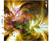 |
Fig. 5 Zoom on NOAA 11589 at 15:00 UT on 2012 October 16, observed with SDO/AIA at 171 Å and overplotted with selected magnetic field lines from the extrapolation (α = 7 × 10⁻³ Mm-1). Blue/green lines are magnetic field lines that give a good/poor match with the AR’s coronal loops. Solid purple/cyan lines display isocontours of the photospheric magnetic field, Bz = [ 30,100,300,1000 ] Gauss. The white arrow indicates the northern direction. |
3.2. QSLs in the active region
3.2.1. QSLs and flare-ribbons
The computation of the squashing degree, Q, in the extrapolation domain was performed using Method 3 of Pariat & Démoulin (2012). Figure 6a displays the photospheric mapping of QSLs by showing log Q at z = 0. Plotting magnetic field lines over the log Q map, we identified three QSLs connected to each other (see Fig. 6). The value of Q in these QSLs is typically about 103−104, which is indicative of strong connectivity gradients. For clarity, these three QSLs are highlighted and labeled Qi (i = { 1,2,3 }) in Fig. 6b. They are respectively compared with the three identified ribbon systems, Ri, in Fig. 6c.
At this point, it must be emphasized again that QSLs depend on the magnetic field connectivity (e.g., Démoulin et al. 1996), which depends on the extrapolation assumptions. This means that extrapolations with different assumptions may lead to different QSLs. In some cases, these QSLs could even disappear. For consistency, we thus reconsidered all the other extrapolations performed, i.e., α = [ −7,−3.5,0,3.5 ] × 10-3 Mm-1, and computed the squashing degree for all of them (see Fig. 7).
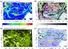 |
Fig. 6 Zoom on NOAA 11589. a) Photospheric mapping of QSLs from the computation of the squashing degree, Q. White regions are related to magnetic field lines that are open on the scale of the extrapolation domain and where Q is not computed. b) Selected magnetic field lines and c) photospheric footprints of the identified QSLs plotted over the photospheric Q-map. The field lines labeled Li = { 1,2,3,4 } indicate possible candidates for the four post-flare loops labeled in Fig. 4. d) Flare ribbons labeled with respect to the identified QSLs footprints. The white arrow indicates the northern direction. |
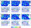 |
Fig. 7 Photospheric mapping of the QSLs of NOAA 11589, from the computation of the squashing degree, Q, for all our LFFF extrapolations. (a), c), e), d), f)) ~ 1 hour before the flare, at 15:00 UT for α = [ 7,3.5,0,−3.5,−7 ] × 10-3 Mm-1. b) ~ 30 min after the flare, at 17:00 UT, for α = 7 × 10⁻³ Mm-1 (i.e., the value considered in this paper). |
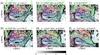 |
Fig. 8 Selected field lines belonging to the three QSLs of NOAA 11589 identified in Fig. 6b, for the same extrapolations as in Fig. 7. Red/orange, dark/light-blue, and green field lines respectively belong to Q1, Q2, and Q3. The gray scale displays the photospheric map of the squashing degree, Q. Solid purple/cyan lines are isocontours of the photospheric vertical magnetic field, Bz = [ 150,300,600 ] Gauss. |
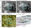 |
Fig. 9 Signatures of magnetic flux emergence occurring in NOAA 11589 around the time of the flare. The cyan rectangle highlights the region of magnetic flux emergence. HMI magnetograms in grayscale a) before the flare, and b) after the flare. The temporal evolution of the magnetograms is available as a movie in the online edition. c) AIA 1600 Å image showing some EBs that are highlighted by the black arrows. d) Extrapolated serpentine field line (green) associated with the EBs shown in Panel c), plotted over the photospheric mapping of the QSLs (grayscale). Solid purple/cyan lines show the same Bz isocontours as in Fig. 5. The white and orange arrows indicate the northern direction. |
The photospheric footprints of QSLs, together with magnetic field line plotting, revealed that these three QSLs are reliable (see Figs. 7 and 8). Indeed, they are present in each considered LFFF extrapolations with similar shapes and locations, meaning that they are topologically robust structures. There are only a few differences that lie on the shapes and intersections of the QSLs footprints. In particular, Figs. 7 and 8 show that while Q2 and Q3 are always connected regardless of the value of the force-free parameter, Q1 and Q2 are solely connected when the force-free parameter of the LFFF extrapolation is positive or zero. From the photospheric mapping of Q (see Fig. 7), it is clear that only LFFF extrapolations with a positive (or null) force-free parameter display QSLs footprints that have a morphology that is compatible with the flare ribbons shown in Figs. 3 and 6. These two figures further justify the use of a positive force-free parameter to analyze the topology of the AR’s magnetic field, and our choice of considering the extrapolation giving the best match with the northern coronal loops where Q1 and the trigger of the flare were located. Among our LFFF extrapolations, we found that the QSLs from the α = 7 × 10⁻³ Mm-1 extrapolation give the best match with the flare ribbons’ shape (see Fig. 6c). We emphasize that a magnetic field extrapolation performed about 30 minutes after the flare, using α = 7 × 10⁻³ Mm-1, further shows that the three identified QSLs were also temporally robust because they subsisted throughout the duration of the flare (see Panels (a) and (c) of Figs. 7 and 8).
Together with magnetic field-line plotting, Fig. 6a allows two double C-shaped QSL footprints, Q{ 1,2 }, and a circular-like QSL, Q3 to be distinguished, in agreement with the three flare ribbons, Ri (see also Fig. 8a). A few discrepancies are found between the QSLs footprints and the flare-ribbons’ shape and location, which results in a rather poor overlay (not shown here). We found the main discrepancies in the identification of Q3,curv and in the relative positions of Q2 and R2. The first is related to the difficulty of distinguishing R3,curv from R1,arc and R2,curv in the AIA 1600 Å images, while it is possible in the extrapolation. The observations tend to suggest that, in the real configuration, Q1,arc, Q2,curv, and Q3,curv are more entangled than in the extrapolation. The second is related to the deformation of R2,arc compared with Q2,arc and to the displacement of R2,curv compared with Q2,curv. The extrapolation shows that Q2,arc is much closer to the PIL than suggested by the corresponding flare ribbon. Also, Q2,curv is very close to the PIL of the northern filament, while the associated ribbon locates it more in the central part between the two filaments.
It is arguable that all these discrepancies are related to the assumption we made by focusing on the large-scale magnetic field of the AR and extrapolating it in LFFF. Indeed, such a hypothesis does not allow the highly-stressed filament magnetic fields and their close surroundings to be modeled. This probably results in local modifications of the connectivity of magnetic field lines, which are responsible for the deformation and displacement of the QSLs in our extrapolation, as compared with the shape and location of the flare ribbons. Nevertheless, distinctive discrepancies between QSLs footprints and flare ribbons can also be found in NLFFF extrapolations. Indeed, this clearly appears in the atypical flare studied by Liu et al. (2014), as can be seen in their Figs. 7d and e. We thus conjecture that such mismatches between QSLs footprints and flare ribbons are more generally inherent to the force-free model of choice.
Despite these discrepancies, we find good qualitative agreement between the QSL footprints and the flare ribbons of our event. This match validates the use of a simplified LFFF model to study the topology of AR 11589 and relate it to the origin of the flare.
Finally, Fig. 6a further exhibits two types of very-high Q regions: the long red stripes closed to the open-field regions (white areas in the Q-map) at the east/west edges of the AR, and the red segments and round shapes. The first are due to the aliasing from the periodic boundary conditions and are spurious. The second are due to very low-altitude null points located above small-scale parasitic polarities. These small QSLs may sustain magnetic reconnection and lead to small-scale jets and bright points. However, they are unrelated to the flare because their field lines do not intersect the QSL system Q1,2,3. We therefore ignore them in our analysis.
3.2.2. A complex interlinked topology
Figure 6b displays a cartoon of the inferred magnetic topology plotted over the photospheric Q-map. It comprises the two double C-shaped QSLs (green and orange QSLs) that resemble the QSL of the quadrupolar magnetic configuration from Titov et al. (2002) or Aulanier et al. (2005). The cartoon also shows that the green and orange QSLs are connected to each other via a third QSL, whose footprints have a very similar shape to the QSL of the null-point configuration studied in Masson et al. (2009) and Reid et al. (2012).
While we did not find any null point associated with Q3, the topology of the magnetic field in the region of Q3,circ, as well as the corresponding circular flare ribbons, are typical signatures of the presence of a magnetic null point (see e.g., Masson et al. 2009; Wang & Liu 2012; Deng et al. 2013). The circular-like shape of the positive magnetic polarity in this region and the low negative magnetic flux suggest the presence of a very low-lying, nearly photospheric null point. The absence of a null point in the corresponding region of our LFFF extrapolation is very likely related to the strength of the magnetic field measured by HMI. Indeed, in the region of Q3, the HMI data display three distinctive negative magnetic polarities whose magnetic field is  , which is lower than the 10 Gauss of HMI sensitivity. We conjecture that the absence of a null point in the corresponding region of our LFFF extrapolation is not inherent to the extrapolation, but is due to a poor precision in the measurement of the weak negative flux – whose strength is comparable to the instrument sensitivity – which prevents retrieving the null.
Overall, the above results show that AR 11589 presents a complex topology that comprises two double C-shaped QSLs, one quasi-separator that links them both (Parnell et al. 2010a), and a possible null point. Such a topology is favorable for the build-up of electric current layers at any of the identified QSLs (e.g., Aulanier et al. 2005; Haynes et al. 2007). Furthermore, any disturbance of any of these topological systems is likely to trigger magnetic reconnection at all the others (e.g., Parnell et al. 2008, 2010b).
4. A confined flare above filaments
4.1. Driver
To identify the possible driver of the observed C3.3 flare, we considered HMI and AIA 1600 Å data sets at a 12-min cadence within a range of four hours prior to and after the flare. Before the flare, the region of the magnetogram enclosed by the cyan rectangle in Fig. 9a displayed spatially aperiodic successions of opposite magnetic polarities in directions oriented from the northeast toward the southwest. These patterns were spatially correlated with Ellerman bombs (EBs; Ellerman 1917) as highlighted in Fig. 9c. EBs are small recurring brightenings often observed in the photospheric wings of chromospheric lines (e.g., Vorpahl & Pope 1972; Kurokawa et al. 1982; Qiu et al. 2000; Georgoulis et al. 2002; Bernasconi et al. 2002; Pariat et al. 2004, 2007; Fang et al. 2006; Bello González et al. 2013; Vissers et al. 2013). They are believed to be the result of bald-patch reconnection occurring along undulatory or serpentine flux tubes as they cross the photosphere and emerge into the solar corona (see Pariat et al. 2004; Cheung et al. 2010). Our LFFF extrapolation suggests that such serpentine flux tubes were indeed present prior to the flare in the region hosting EBs, as shown Fig. 9d. Finally, Fig. 9b shows that a new bipole appeared some time after the flare, as inferred from the broad patches of opposite polarities present in the center of the cyan rectangle and which are accompanied with small-scale bipolar patches.
Such observational features are clear signatures of magnetic flux emergence starting hours before the flare onset. This emergence occurred below the QSL Q1, in between the western part of the Q1,curv and the southern part of the Q1,arc branches. Furthermore, this region below Q1 corresponds to the location of the first flare brightenings. This continuous emergence below Q1 may well have induced magnetic reconnection at this QSL. It may thus have been responsible for the trigger of the flare (e.g., Schmieder et al. 1997; Bagalá et al. 2000; del Zanna et al. 2006). We therefore conjecture that continuous emergence starting prior to the flare and occurring below the northern QSL of the AR was the driver of the observed C-class flare.
4.2. Proposed flare scenario
We propose that the observed C-class flare was the result of a multiple-step reconnection mechanism driven by magnetic flux emergence below Q1. In this scenario, the continuous magnetic flux emergence below Q1 leads to the accumulation of magnetic stress at Q1, which results in the build-up of an electric current layer at this QSL (e.g., Milano et al. 1999; Aulanier et al. 2005; Török et al. 2009). This emergence leads to the intensification and the thinning of this current layer, which eventually triggers slipping/slip-running magnetic reconnection (Aulanier et al. 2006b), at Q1, of the emerging field with the ambient pre-existing magnetic field.
Because of the proximity of Q1,arc with Q2,curv and Q3,curv, or Q1,curv with Q2,arc and Q3,circ, the slipping/slip-running magnetic reconnection at Q1 is likely to stress the magnetic field of Q2 and Q3 since magnetic stress can be transported at all QSLs via the quasi-separator that links the QSLs all together (e.g., Priest & Titov 1996; Galsgaard & Nordlund 1997; Parnell et al. 2008). Indeed, at the quasi separator, the QSLs share common magnetic field lines. The stress of such field lines at one of the QSLs is thus likely to also build-up stress at the quasi-separator and/or at the other QSL(s) sharing these field lines. Such a stress may build up electric currents at Q2 and Q3 or may increase pre-existing electric currents within these two QSLs. Eventually, the induced stress of Q2 and/or Q3 triggers magnetic reconnection at these two QSLs.
In our scenario, the flare is thus the consequence of continuous slow emergence of magnetic flux below Q1, which results in slipping/slip-running reconnection at this QSL, eventually triggering reconnection at the two other interlinked QSLs. Particle acceleration is thus expected at all QSLs, implying the formation of flare ribbons at all QSLs footprints and of post-flare loops anchored in the flare-ribbons (e.g., Gorbachev & Somov 1989; Schmieder et al. 1997; Mandrini et al. 2006; Baker et al. 2009; Chandra et al. 2011), as supported by the AIA 1600 and 193 Å data in Figs. 6 and 4 in this particular event.
It must be emphasized that all three QSLs involved in our flare scenario are located above the two observed non-eruptive filaments, which are passive during the flare that spreads in the corona above and around them. This a posteriori supports the assumption made in Sect. 3.1 that the flare mechanism did not involve the magnetic field of the filaments. Our scenario thus explains the formation of the two extended flare ribbons around the two filaments, as the consequence of sequential magnetic reconnection occurring in a complex system of three interlinked QSLs located above the filaments.
5. Summary and discussion
In this study, we used multiwavelength, high-resolution observations obtained by the SDO, ARIES, and THEMIS instruments, so as to analyze the dynamics of the magnetic field of AR NOAA 11589 that led to a non-standard C3.3 class flare on 2012 October 16. The AR evolution was associated with large-scale magnetic flux cancellation that led to the formation of two filaments of opposite chirality. Unlike what the standard model predicts, the flare loops formed above and not below the filaments. Furthermore, the latter were apparently not involved in the flare mechanism, since they did not erupt. The dataset considered here also presented the signatures of localized magnetic flux emergence episodes in the northern part of the AR. Our analysis indicates that the flare was driven by one of these episodes that actually took place below a complex system of quasi-separatrix layers (QSLs), as calculated in a linear force-free field (LFFF) extrapolation. This continuous magnetic flux emergence presumably stressed the magnetic field of the QSLs, thus resulting in the development of narrow and intense current layers within them. This scenario implies the occurrence of multiple and sequential magnetic reconnections within the complex set of QSLs, which led to the observed flare. This scenario is supported by the relatively good match found between the expected timing of the QSL activations, the shape of the QSL footprints, and the development and morphology of complex flare ribbons and loops as observed in the EUV (see the online movie associated with Fig. 3).
By performing a set of LFFF extrapolations using different values of the force-free parameter, we have demonstrated the robustness of the derived complex topology, hence of our results. More generally, our study shows the stability of the QSLs related to large-scale coronal loops/magnetic fields that are not associated with a magnetic flux rope. In particular, it shows the stability of such QSLs (1) against changes – within a certain range – of the force-free parameter for LFFF extrapolations (see also Aulanier et al. 2005), and (2) against temporal variations that do not result in a major evolution of the photospheric magnetic flux and/or of electric currents (see also the large-scale QSL of the quadrupolar AR 11158 in Zhao et al. 2014). We recall that the force-free parameter controls the amount of electric current density in magnetic field lines, which can be observationally related to the photospheric transverse/horizontal magnetic field. Therefore, the stability of the QSLs of large-scale coronal loops/magnetic fields – not associated with a magnetic flux-rope – suggests that such QSLs are mainly constrained by the photospheric longitudinal/vertical magnetic field, hence, by the large-scale distribution of the photospheric magnetic flux.
It is worth noticing that the flare scenario that we proposed is based on one important conjecture, namely that slip-running reconnection may activate several QSLs that are linked. This may be expected because reconnecting field lines may slip from one QSL to another. In this picture, a given field line may reconnect at least two times in the considered magnetic configuration. Such sequences of magnetic reconnections for a given field line have already been reported for magnetic configurations with separatrices intersecting at a separator (e.g., Galsgaard & Nordlund 1997; Haynes et al. 2007; Parnell et al. 2010a). However, to the authors’ knowledge, it has never been shown to occur in complex QSL systems in which two QSLs are located in the vicinity of one another. Therefore, this conjecture should be addressed by future numerical experiments in which the initial magnetic field configurations should possess two neighboring QSLs.
The C3.3 class flare analyzed in this paper is a typical example of an atypical flare exhibiting signatures common to both standard and confined solar flares. Indeed, on large scales, the flare initially appears to be associated with the formation of two extended ribbons that developed parallel to and next to the filaments, in a generally bipolar active region, as in in the standard model. However, on smaller scales, the polarity inversion line is strongly curved. The ribbons have a complex shape, and they did not brighten simultaneously. Together, these two features suggest some coupling of remote regions that did not seem to be magnetically linked to the filaments. Furthermore, the filaments did not erupt either, nor were they associated with any failed eruption. Explaining this type of atypical event in general may be a challenge for the usual eruptive and confined flare models. Nevertheless, the topological analysis of the magnetic field derived from a force-free extrapolation, here achieved using the QSL method (applied with the squashing degree, Q; Démoulin et al. 1997), shows that it is possible to explain atypical flare signatures as a complex QSL system that allows coupling remote regions via slip-running reconnection (Aulanier et al. 2006b).
On the one hand, this work further confirms that QSLs play a key role in 3D reconnection in solar flares, as reported in previous studies of less complex events (e.g., Schmieder et al. 1997; Mandrini et al. 2006; Chandra et al. 2011). On the other hand, this study suggests that topological analyses, such as the QSL method (using either N or Q), may also be the way to explain atypical solar flares, which may actually be more numerous than the more classical eruptive and confined flares that are often analyzed in the literature. This conclusion is further confirmed by the topological analysis of a different atypical flare studied in the framework of the QSL method by Liu et al. (2014). In their event, the magnetic configuration was derived using a nonlinear force-free field (NLFFF) extrapolation. Similar to our event, the derived configuration possessed a large-scale QSL above a magnetic flux rope (although our event was associated with two QSLs and two filaments, each QSL lying above a filament). As in our case, the flare was very likely driven by magnetic flux emergence occurring below the large-scale QSL, in a different region from the flux-rope location, and it eventually triggered magnetic reconnection at this QSL. However, unlike our event, the continuous reconnection at the large-scale QSL of their configuration eventually destabilized the flux rope whose eruption failed due to the presence of strong confining arcades above it.
If atypical solar flares are the most numerous, then the study by Liu et al. (2014) and ours suggest that the classical paradigm of confined and eruptive flares should be revisited. However, these are only two independent case studies, so further topological analyses of atypical solar flares, using either LFFF or NLFFF extrapolations, are required to confirm such a statement, and to confirm that topological studies are indeed relevant for all these complex events.
Online material
Movie of Fig. 1 Access Supplementary Material
Movie of Fig. 3 Access Supplementary Material
Movie of Fig. 9 Access Supplementary Material
Acknowledgments
We thank the referee for helpful comments that improved the paper. We deeply thank Dr. W. Uddin for providing us with the observations of the ARIES telescope. We thank all the team of THEMIS for adjusting the telescope during our observing campaign and the director, Bernard Gelly for providing us with the data. K.D. thanks E. Pariat for fruitful discussions that helped in identifying the driver of the flare. R.C. thanks the Observatoire de Paris for the grant given during his stay in Meudon in January 2013. We acknowledge the open data policy of NASA/SDO.
References
- Alissandrakis, C. E. 1981, A&A, 100, 197 [NASA ADS] [Google Scholar]
- Aly, J. J., & Amari, T. 1997, A&A, 319, 699 [NASA ADS] [Google Scholar]
- Antiochos, S. K., Dahlburg, R. B., & Klimchuk, J. A. 1994, ApJ, 420, L41 [Google Scholar]
- Aulanier, G. 2011, in IAU Symp., 273, eds. D. Prasad Choudhary, & K. G. Strassmeier, 233 [Google Scholar]
- Aulanier, G., & Démoulin, P. 1998, A&A, 329, 1125 [Google Scholar]
- Aulanier, G., Pariat, E., & Démoulin, P. 2005, A&A, 444, 961 [NASA ADS] [CrossRef] [EDP Sciences] [Google Scholar]
- Aulanier, G., DeVore, C. R., & Antiochos, S. K. 2006a, ApJ, 646, 1349 [NASA ADS] [CrossRef] [Google Scholar]
- Aulanier, G., Pariat, E., Démoulin, P., & DeVore, C. R. 2006b, Sol. Phys., 238, 347 [NASA ADS] [CrossRef] [Google Scholar]
- Aulanier, G., Janvier, M., & Schmieder, B. 2012, A&A, 543, A110 [NASA ADS] [CrossRef] [EDP Sciences] [Google Scholar]
- Bagalá, L. G., Mandrini, C. H., Rovira, M. G., & Démoulin, P. 2000, A&A, 363, 779 [NASA ADS] [Google Scholar]
- Baker, D., van Driel-Gesztelyi, L., Mandrini, C. H., Démoulin, P., & Murray, M. J. 2009, ApJ, 705, 926 [Google Scholar]
- Bello González, N., Danilovic, S., & Kneer, F. 2013, A&A, 557, A102 [NASA ADS] [CrossRef] [EDP Sciences] [Google Scholar]
- Bernasconi, P. N., Rust, D. M., Georgoulis, M. K., & Labonte, B. J. 2002, Sol. Phys., 209, 119 [NASA ADS] [CrossRef] [Google Scholar]
- Canou, A., & Amari, T. 2010, ApJ, 715, 1566 [NASA ADS] [CrossRef] [Google Scholar]
- Carmichael, H. 1964, NASA Sp. Publ., 50, 451 [Google Scholar]
- Chandra, R., Jain, R., Uddin, W., et al. 2006, Sol. Phys., 239, 239 [NASA ADS] [CrossRef] [Google Scholar]
- Chandra, R., Schmieder, B., Aulanier, G., & Malherbe, J. M. 2009, Sol. Phys., 258, 53 [NASA ADS] [CrossRef] [Google Scholar]
- Chandra, R., Pariat, E., Schmieder, B., Mandrini, C. H., & Uddin, W. 2010, Sol. Phys., 261, 127 [NASA ADS] [CrossRef] [Google Scholar]
- Chandra, R., Schmieder, B., Mandrini, C. H., et al. 2011, Sol. Phys., 269, 83 [NASA ADS] [CrossRef] [Google Scholar]
- Chen, H., Ma, S., & Zhang, J. 2013, ApJ, 778, 70 [NASA ADS] [CrossRef] [Google Scholar]
- Cheung, M. C. M., Rempel, M., Title, A. M., & Schüssler, M. 2010, ApJ, 720, 233 [NASA ADS] [CrossRef] [Google Scholar]
- del Zanna, G., Berlicki, A., Schmieder, B., & Mason, H. E. 2006, Sol. Phys., 234, 95 [NASA ADS] [CrossRef] [Google Scholar]
- Démoulin, P. 2006, Adv. Space Res., 37, 1269 [NASA ADS] [CrossRef] [Google Scholar]
- Démoulin, P. 2007, Adv. Space Res., 39, 1367 [NASA ADS] [CrossRef] [Google Scholar]
- Démoulin, P., Priest, E. R., & Anzer, U. 1989, A&A, 221, 326 [NASA ADS] [Google Scholar]
- Démoulin, P., Priest, E. R., & Lonie, D. P. 1996, J. Geophys. Res., 101, 7631 [NASA ADS] [CrossRef] [Google Scholar]
- Démoulin, P., Bagala, L. G., Mandrini, C. H., Henoux, J. C., & Rovira, M. G. 1997, A&A, 325, 305 [NASA ADS] [Google Scholar]
- Deng, Y., Lin, Y., Schmieder, B., & Engvold, O. 2002, Sol. Phys., 209, 153 [Google Scholar]
- Deng, N., Tritschler, A., Jing, J., et al. 2013, ApJ, 769, 112 [NASA ADS] [CrossRef] [Google Scholar]
- DeVore, C. R., Antiochos, S. K., & Aulanier, G. 2005, ApJ, 629, 1122 [NASA ADS] [CrossRef] [Google Scholar]
- Ellerman, F. 1917, ApJ, 46, 298 [NASA ADS] [CrossRef] [Google Scholar]
- Fang, C., Tang, Y. H., Xu, Z., Ding, M. D., & Chen, P. F. 2006, ApJ, 643, 1325 [NASA ADS] [CrossRef] [Google Scholar]
- Forbes, T. G., & Malherbe, J. M. 1986, ApJ, 302, L67 [NASA ADS] [CrossRef] [Google Scholar]
- Galsgaard, K., & Nordlund, Å. 1997, J. Geophys. Res., 102, 231 [NASA ADS] [CrossRef] [Google Scholar]
- Gekelman, W., Lawrence, E., & Van Compernolle, B. 2012, ApJ, 753, 131 [NASA ADS] [CrossRef] [Google Scholar]
- Georgoulis, M. K., Rust, D. M., Bernasconi, P. N., & Schmieder, B. 2002, ApJ, 575, 506 [NASA ADS] [CrossRef] [Google Scholar]
- Giovanelli, R. G. 1947, MNRAS, 107, 338 [NASA ADS] [CrossRef] [Google Scholar]
- Gorbachev, V. S., & Somov, B. V. 1989, Sov. Ast, 33, 57 [Google Scholar]
- Green, L. M., López fuentes, M. C., Mandrini, C. H., et al. 2002, Sol. Phys., 208, 43 [NASA ADS] [CrossRef] [Google Scholar]
- Guo, Y., Ding, M. D., Schmieder, B., et al. 2010, ApJ, 725, L38 [NASA ADS] [CrossRef] [Google Scholar]
- Guo, Y., Ding, M. D., Liu, Y., et al. 2012, ApJ, 760, 47 [NASA ADS] [CrossRef] [Google Scholar]
- Hanaoka, Y. 1997, Sol. Phys., 173, 319 [NASA ADS] [CrossRef] [Google Scholar]
- Haynes, A. L., Parnell, C. E., Galsgaard, K., & Priest, E. R. 2007, Royal Society of London Proceedings Series A, 463, 1097 [Google Scholar]
- Heyvaerts, J., Priest, E. R., & Rust, D. M. 1977, ApJ, 216, 123 [NASA ADS] [CrossRef] [Google Scholar]
- Hirayama, T. 1974, Sol. Phys., 34, 323 [NASA ADS] [CrossRef] [Google Scholar]
- Janvier, M., Aulanier, G., Pariat, E., & Démoulin, P. 2013, A&A, 555, A77 [NASA ADS] [CrossRef] [EDP Sciences] [Google Scholar]
- Jiang, C., & Feng, X. 2013, ApJ, 769, 144 [NASA ADS] [CrossRef] [Google Scholar]
- Kopp, R. A., & Pneuman, G. W. 1976, Sol. Phys., 50, 85 [NASA ADS] [CrossRef] [Google Scholar]
- Kurokawa, H., Kawaguchi, I., Funakoshi, Y., & Nakai, Y. 1982, Sol. Phys., 79, 77 [NASA ADS] [CrossRef] [Google Scholar]
- Kusano, K., Bamba, Y., Yamamoto, T. T., et al. 2012, ApJ, 760, 31 [NASA ADS] [CrossRef] [Google Scholar]
- Lawrence, E. E., & Gekelman, W. 2009, Phys. Rev. Lett., 103, 105002 [NASA ADS] [CrossRef] [Google Scholar]
- Leka, K. D., & Skumanich, A. 1999, Sol. Phys., 188, 3 [NASA ADS] [CrossRef] [Google Scholar]
- Lemen, J. R., Title, A. M., Akin, D. J., et al. 2012, Sol. Phys., 275, 17 [NASA ADS] [CrossRef] [Google Scholar]
- Liu, R., Titov, V. S., Gou, T., et al. 2014, ApJ, 790, 8 [NASA ADS] [CrossRef] [Google Scholar]
- Longcope, D. W. 2005, Living Rev. Sol. Phys., 2, 7 [Google Scholar]
- Low, B. C., & Wolfson, R. 1988, ApJ, 324, 574 [NASA ADS] [CrossRef] [Google Scholar]
- Mackay, D. H., Karpen, J. T., Ballester, J. L., Schmieder, B., & Aulanier, G. 2010, Space Sci. Rev., 151, 333 [NASA ADS] [CrossRef] [Google Scholar]
- Maia, D., Aulanier, G., Wang, S. J., et al. 2003, A&A, 405, 313 [NASA ADS] [CrossRef] [EDP Sciences] [Google Scholar]
- Mandrini, C. H., Démoulin, P., Bagala, L. G., et al. 1997, Sol. Phys., 174, 229 [NASA ADS] [CrossRef] [Google Scholar]
- Mandrini, C. H., Démoulin, P., Schmieder, B., et al. 2006, Sol. Phys., 238, 293 [NASA ADS] [CrossRef] [Google Scholar]
- Martens, P. C., & Zwaan, C. 2001, ApJ, 558, 872 [Google Scholar]
- Martin, S. F. 1998, Sol. Phys., 182, 107 [NASA ADS] [CrossRef] [Google Scholar]
- Masson, S., Pariat, E., Aulanier, G., & Schrijver, C. J. 2009, ApJ, 700, 559 [NASA ADS] [CrossRef] [Google Scholar]
- Masson, S., Aulanier, G., Pariat, E., & Klein, K.-L. 2012, Sol. Phys., 276, 199 [NASA ADS] [CrossRef] [Google Scholar]
- McClymont, A. N., Jiao, L., & Mikic, Z. 1997, Sol. Phys., 174, 191 [NASA ADS] [CrossRef] [Google Scholar]
- Milano, L. J., Dmitruk, P., Mandrini, C. H., Gómez, D. O., & Démoulin, P. 1999, ApJ, 521, 889 [NASA ADS] [CrossRef] [Google Scholar]
- Moore, R. L., Sterling, A. C., Hudson, H. S., & Lemen, J. R. 2001, ApJ, 552, 833 [NASA ADS] [CrossRef] [Google Scholar]
- Nakagawa, Y., & Raadu, M. A. 1972, Sol. Phys., 25, 127 [NASA ADS] [CrossRef] [Google Scholar]
- Nishio, M., Yaji, K., Kosugi, T., Nakajima, H., & Sakurai, T. 1997, ApJ, 489, 976 [NASA ADS] [CrossRef] [Google Scholar]
- Pariat, E., & Démoulin, P. 2012, A&A, 541, A78 [NASA ADS] [CrossRef] [EDP Sciences] [Google Scholar]
- Pariat, E., Aulanier, G., Schmieder, B., et al. 2004, ApJ, 614, 1099 [Google Scholar]
- Pariat, E., Schmieder, B., Berlicki, A., et al. 2007, A&A, 473, 279 [NASA ADS] [CrossRef] [EDP Sciences] [Google Scholar]
- Parnell, C. E., Haynes, A. L., & Galsgaard, K. 2008, ApJ, 675, 1656 [NASA ADS] [CrossRef] [Google Scholar]
- Parnell, C. E., Haynes, A. L., & Galsgaard, K. 2010a, J. Geophys. Res. (Space Phys.), 115, 2102 [Google Scholar]
- Parnell, C. E., Maclean, R. C., & Haynes, A. L. 2010b, ApJ, 725, L214 [NASA ADS] [CrossRef] [Google Scholar]
- Pesnell, W. D., Thompson, B. J., & Chamberlin, P. C. 2012, Sol. Phys., 275, 3 [NASA ADS] [CrossRef] [Google Scholar]
- Pevtsov, A. A., Balasubramaniam, K. S., & Rogers, J. W. 2003, ApJ, 595, 500 [NASA ADS] [CrossRef] [Google Scholar]
- Priest, E. R., & Démoulin, P. 1995, J. Geophys. Res., 100, 23443 [NASA ADS] [CrossRef] [Google Scholar]
- Priest, E. R., & Forbes, T. G. 1992, J. Geophys. Res., 97, 1521 [NASA ADS] [CrossRef] [Google Scholar]
- Priest, E. R., & Forbes, T. G. 2002, A&A Rev., 10, 313 [Google Scholar]
- Priest, E. R., & Titov, V. S. 1996, Roy. Soc. London Philos. Trans. Ser. A, 354, 2951 [Google Scholar]
- Qiu, J., Ding, M. D., Wang, H., Denker, C., & Goode, P. R. 2000, ApJ, 544, L157 [NASA ADS] [CrossRef] [Google Scholar]
- Régnier, S. 2013, Sol. Phys., 288, 481 [NASA ADS] [CrossRef] [Google Scholar]
- Reid, H. A. S., Vilmer, N., Aulanier, G., & Pariat, E. 2012, A&A, 547, A52 [NASA ADS] [CrossRef] [EDP Sciences] [Google Scholar]
- Savcheva, A., Pariat, E., van Ballegooijen, A., Aulanier, G., & DeLuca, E. 2012, ApJ, 750, 15 [NASA ADS] [CrossRef] [Google Scholar]
- Schmieder, B., Heinzel, P., Wiik, J. E., et al. 1995, Sol. Phys., 156, 337 [NASA ADS] [CrossRef] [Google Scholar]
- Schmieder, B., Heinzel, P., van Driel-Gesztelyi, L., & Lemen, J. R. 1996, Sol. Phys., 165, 303 [NASA ADS] [CrossRef] [Google Scholar]
- Schmieder, B., Aulanier, G., Demoulin, P., et al. 1997, A&A, 325, 1213 [NASA ADS] [Google Scholar]
- Schmieder, B., Mein, N., Deng, Y., et al. 2004, Sol. Phys., 223, 119 [NASA ADS] [CrossRef] [Google Scholar]
- Schou, J., Borrero, J. M., Norton, A. A., et al. 2012, Sol. Phys., 275, 327 [NASA ADS] [CrossRef] [Google Scholar]
- Schrijver, C. J., De Rosa, M. L., Metcalf, T., et al. 2008, ApJ, 675, 1637 [Google Scholar]
- Shibata, K. 1999, Ap&SS, 264, 129 [NASA ADS] [CrossRef] [Google Scholar]
- Shibata, K., & Magara, T. 2011, Liv. Rev. Sol. Phys., 8, 6 [Google Scholar]
- Shibata, K., Masuda, S., Shimojo, M., et al. 1995, ApJ, 451, L83 [NASA ADS] [CrossRef] [Google Scholar]
- Sturrock, P. A. 1966, Nature, 211, 695 [NASA ADS] [CrossRef] [Google Scholar]
- Syrovatskii, S. I. 1981, ARA&A, 19, 163 [NASA ADS] [CrossRef] [Google Scholar]
- Titov, V. S., Hornig, G., & Démoulin, P. 2002, J. Geophys. Res., 107, 1164 [Google Scholar]
- Török, T., & Kliem, B. 2005, ApJ, 630, L97 [Google Scholar]
- Török, T., Aulanier, G., Schmieder, B., Reeves, K. K., & Golub, L. 2009, ApJ, 704, 485 [NASA ADS] [CrossRef] [Google Scholar]
- Török, T., Chandra, R., Pariat, E., et al. 2011, ApJ, 728, 65 [NASA ADS] [CrossRef] [Google Scholar]
- Valori, G., Green, L. M., Démoulin, P., et al. 2012, Sol. Phys., 278, 73 [NASA ADS] [CrossRef] [Google Scholar]
- van Ballegooijen, A. A., & Martens, P. C. H. 1989, ApJ, 343, 971 [NASA ADS] [CrossRef] [Google Scholar]
- Vissers, G. J. M., Rouppe van der Voort, L. H. M., & Rutten, R. J. 2013, ApJ, 774, 32 [NASA ADS] [CrossRef] [Google Scholar]
- Vorpahl, J., & Pope, T. 1972, Sol. Phys., 25, 347 [NASA ADS] [CrossRef] [Google Scholar]
- Wang, H., & Liu, C. 2012, ApJ, 760, 101 [NASA ADS] [CrossRef] [Google Scholar]
- Wang, Y.-M., & Muglach, K. 2007, ApJ, 666, 1284 [NASA ADS] [CrossRef] [Google Scholar]
- Wiegelmann, T. 2004, Sol. Phys., 219, 87 [NASA ADS] [CrossRef] [Google Scholar]
- Wiegelmann, T., & Sakurai, T. 2012, Liv. Rev. Sol. Phys., 9, 5 [Google Scholar]
- Wiegelmann, T., Thalmann, J. K., Inhester, B., et al. 2012, Sol. Phys., 281, 37 [NASA ADS] [Google Scholar]
- Wilmot-Smith, A. L., Pontin, D. I., & Hornig, G. 2010, A&A, 516, A5 [NASA ADS] [CrossRef] [EDP Sciences] [Google Scholar]
- Zhao, J., Li, H., Pariat, E., et al. 2014, ApJ, 787, 88 [NASA ADS] [CrossRef] [Google Scholar]
All Figures
|
Fig. 1 Evolution of active region NOAA 11589 during its disk passage before the eruption on 2012 October 16. Top: evolution of the longitudinal magnetic field observed by SDO/HMI. White/black are positive/negative polarities. The field strength is saturated at 500 Gauss. The violet arrows indicate significant emerging fluxes on October 13 and 15. The cyan rectangle highlights the region where recurring magnetic flux emergence occurred on October 16 and likely triggered the studied C3-class flare (see Sect. 2.4). The temporal evolution of the magnetograms is available as a movie in the online edition. Bottom: development of filaments in Hα observed by ARIES telescope. The locations of two observed filaments F1 and F2 are indicated by black arrows. The white arrow indicates the north direction. |
| In the text | |
|
Fig. 2 Active region NOAA 11589 observed on 2012 October 16 by THEMIS/MTR between 08:02 and 09:02 UT. Top: longitudinal magnetic field. Bottom: Hα map showing the two recently formed filaments of Fig. 1. The white arrows indicate the barbs used to infer the filaments’ chirality. Filament F1 is a dextral filament and F2 is a sinistral filament. The + and − signs indicate the magnetic field polarity of each end of the filaments. The field of view covers ~ 175′′ × 100′′. The white arrow indicates the north direction. |
| In the text | |
|
Fig. 3 Flare signatures observed by SDO/AIA on 2012 October 16 at 1600 Å (left), at 304 Å (middle), and at 171 Å (right). The black arrow indicates the northern direction. The white square indicates the field of view of Fig. 4. The temporal evolution of AIA 1600 Å, 304 Å, and 171 Å images is available as a movie in the online edition. |
| In the text | |
|
Fig. 4 Flare signatures observed by SDO/AIA on 2012 October 16 at 193 Å. In the top left panel, the white arrow indicates the northern direction. |
| In the text | |
|
Fig. 5 Zoom on NOAA 11589 at 15:00 UT on 2012 October 16, observed with SDO/AIA at 171 Å and overplotted with selected magnetic field lines from the extrapolation (α = 7 × 10⁻³ Mm-1). Blue/green lines are magnetic field lines that give a good/poor match with the AR’s coronal loops. Solid purple/cyan lines display isocontours of the photospheric magnetic field, Bz = [ 30,100,300,1000 ] Gauss. The white arrow indicates the northern direction. |
| In the text | |
|
Fig. 6 Zoom on NOAA 11589. a) Photospheric mapping of QSLs from the computation of the squashing degree, Q. White regions are related to magnetic field lines that are open on the scale of the extrapolation domain and where Q is not computed. b) Selected magnetic field lines and c) photospheric footprints of the identified QSLs plotted over the photospheric Q-map. The field lines labeled Li = { 1,2,3,4 } indicate possible candidates for the four post-flare loops labeled in Fig. 4. d) Flare ribbons labeled with respect to the identified QSLs footprints. The white arrow indicates the northern direction. |
| In the text | |
|
Fig. 7 Photospheric mapping of the QSLs of NOAA 11589, from the computation of the squashing degree, Q, for all our LFFF extrapolations. (a), c), e), d), f)) ~ 1 hour before the flare, at 15:00 UT for α = [ 7,3.5,0,−3.5,−7 ] × 10-3 Mm-1. b) ~ 30 min after the flare, at 17:00 UT, for α = 7 × 10⁻³ Mm-1 (i.e., the value considered in this paper). |
| In the text | |
|
Fig. 8 Selected field lines belonging to the three QSLs of NOAA 11589 identified in Fig. 6b, for the same extrapolations as in Fig. 7. Red/orange, dark/light-blue, and green field lines respectively belong to Q1, Q2, and Q3. The gray scale displays the photospheric map of the squashing degree, Q. Solid purple/cyan lines are isocontours of the photospheric vertical magnetic field, Bz = [ 150,300,600 ] Gauss. |
| In the text | |
|
Fig. 9 Signatures of magnetic flux emergence occurring in NOAA 11589 around the time of the flare. The cyan rectangle highlights the region of magnetic flux emergence. HMI magnetograms in grayscale a) before the flare, and b) after the flare. The temporal evolution of the magnetograms is available as a movie in the online edition. c) AIA 1600 Å image showing some EBs that are highlighted by the black arrows. d) Extrapolated serpentine field line (green) associated with the EBs shown in Panel c), plotted over the photospheric mapping of the QSLs (grayscale). Solid purple/cyan lines show the same Bz isocontours as in Fig. 5. The white and orange arrows indicate the northern direction. |
| In the text | |
Current usage metrics show cumulative count of Article Views (full-text article views including HTML views, PDF and ePub downloads, according to the available data) and Abstracts Views on Vision4Press platform.
Data correspond to usage on the plateform after 2015. The current usage metrics is available 48-96 hours after online publication and is updated daily on week days.
Initial download of the metrics may take a while.