| Issue |
A&A
Volume 573, January 2015
|
|
|---|---|---|
| Article Number | A18 | |
| Number of page(s) | 11 | |
| Section | Stellar structure and evolution | |
| DOI | https://doi.org/10.1051/0004-6361/201424957 | |
| Published online | 09 December 2014 | |
Pulsations of red supergiant pair-instability supernova progenitors leading to extreme mass loss
Argelander Institute for Astronomy, University of Bonn,
Auf dem Hügel 71,
53121
Bonn,
Germany
e-mail:
This email address is being protected from spambots. You need JavaScript enabled to view it.
Received: 11 September 2014
Accepted: 15 October 2014
Abstract
Recent stellar evolution models show consistently that very massive metal-free stars evolve into red supergiants shortly before they explode. We argue that the envelopes of these stars, which will form pair-instability supernovae, become pulsationally unstable and that this will lead to extreme mass-loss rates despite the tiny metal content of the envelopes. We investigate the pulsational properties of such models and derive pulsationally induced mass-loss rates, which take the damping effects of the mass loss on the pulsations selfconsistently into account. We find that the pulsations may induce mass-loss rates of ~10-4 − 10-2M⊙ yr-1 shortly before the explosions, which may create a dense circumstellar medium. Our results show that very massive stars with dense circumstellar media may stem from a wider initial mass range than pulsational-pair instability supernovae. The extreme mass loss will cease when so much of the hydrogen-rich envelope is lost that the star becomes more compact and stops pulsating. The helium core of these stars therefore remains unaffected, and their fate as pair-instability supernovae remains unaltered. The existence of dense circumstellar media around metal-free pair-instability supernovae can make them brighter and bluer, and they may be easier to detect at high redshifts than previously expected. We argue that the mass-loss enhancement in pair-instability supernova progenitors can naturally explain some observational properties of superluminous supernovae: the energetic explosions of stars within hydrogen-rich dense circumstellar media with little 56Ni production and the lack of a hydrogen-rich envelope in pair-instability supernova candidates with large 56Ni production.
Key words: stars: evolution / stars: massive / stars: mass-loss / supernovae: general
© ESO, 2014
1. Introduction
Pair-instability supernovae (PISNe) are theoretically predicted explosions of very massive stars that are triggered by the creation of electron-positron pairs in their cores (e.g., Rakavy & Shaviv 1967; Barkat et al. 1967). The pair creation makes very massive stars dynamically unstable and leads to their collapse. The collapse triggers explosive nuclear burning, thereby unbinding the entire star. PISNe can be very bright because of their huge explosion energy and large 56Ni production (e.g., Kasen et al. 2011; Dessart et al. 2013; Whalen et al. 2013; Kozyreva et al. 2014). PISNe have long remained a theoretical prediction, but several possible observational candidates have been discovered recently (e.g., Gal-Yam et al. 2009). The predicted characteristic chemical signatures of PISNe (e.g., Heger & Woosley 2002) have not yet been observed in metal-poor stars (e.g., Yong et al. 2013), although a potential candidate metal-poor star showing such a signature has been reported recently (Aoki et al. 2014).
Properties of our stellar models.
Strong mass loss on the main sequence or thereafter may lead to lower core masses, thereby preventing very massive stars developing the pair instability. Thus, PISNe are likely to occur where the mass-loss rates can be low (e.g., Heger & Woosley 2002; Umeda & Nomoto 2002; Langer et al. 2007; Yoon et al. 2012; Yusof et al. 2013; Yoshida et al. 2014), i.e., at low metallicity. Especially, the first zero-metallicity stars are said to form very massive stars primarily, possibly producing PISNe due to the lack of radiation-driven mass loss (e.g., Hirano et al. 2014; Susa et al. 2014). Despite their low metallicity, stars that are slightly less massive than PISN progenitors are able to experience a large amount of mass loss very late in their evolution (e.g., Woosley et al. 2007; Ohkubo et al. 2009; Chatzopoulos & Wheeler 2012a,b). This is because the pair instability occurs in these stars, but it is so weak that they are only partially disrupted. The successive eruptions of these stars may produce a dense circumstellar medium (CSM), which may explain the high luminosities in some superluminous SNe (SLSNe, Woosley et al. 2007; Whalen et al. 2014; Chen et al. 2014). Even though these luminous transients are likely not accompanied by SNe since the stars eventually collapse to form a black hole, they are called pulsational pair-instability SNe.
An interesting property of PISN progenitors displayed by stellar evolution models is that many of them are red supergiants (RSGs) when they explode (e.g., Langer et al. 2007; Yoon et al. 2012; Dessart et al. 2013). An important property of RSGs that has not been taken into account in the PISN progenitor modeling is that hydrogen-rich envelopes of RSGs are pulsationally unstable when their L/M-ratio is high, where L is the stellar luminosity and M the stellar mass (Li & Gong 1994; Heger et al. 1997; Yoon & Cantiello 2010). The fundamental mode of the radial pulsations is said to grow in RSGs due to the κ mechanism working at the hydrogen ionization zones in the RSG envelopes.
Pulsational properties of metal-free very massive stars have been investigated by Baraffe et al. (2001). While they were found to be pulsationally unstable on the main sequence, Baraffe et al. (2001) conclude from the tiny growth rates of the pulsations that any effect on the mass-loss rates would be negligible (see also Sonoi & Umeda 2012). Their most massive models (300 and 500 M⊙) evolved into RSGs at the end of their evolution, and while they noted that the models became more violently pulsationally unstable during that stage, they did not investigate this any further.
Various authors suggested that for large enough amplitudes, pulsations may induce stellar mass loss (e.g., Appenzeller 1970a,b; Bowen 1988; Höfner et al. 2003; Neilson & Lester 2008). For example, pulsations are known to be an essential driver of the mass loss in carbon-rich asymptotic giant-branch stars. The pulsations create high-density regions above the stellar photosphere in which dust can be formed. Thanks to the high opacity of the formed dust, their mass-loss rates are enhanced significantly (e.g., Höfner et al. 2003; Höfner 2008; Wood 1979). The large mass loss induced by pulsations in the RSG stage was said to influence the final fates of massive stars (e.g., Heger et al. 1997; Yoon & Cantiello 2010; Moriya et al. 2011; Georgy 2012). Previous studies of RSG pulsations focussed on core-collapse SN progenitors below 40 M⊙ (Heger et al. 1997; Yoon & Cantiello 2010).
In this paper, we investigate the pulsational properties of massive metal-free PISN progenitors (150 − 250 M⊙) during their RSG stage. After introducing our methods to follow the stellar evolution in Sect. 2, we show that these stars are pulsationally unstable, discuss their pulsational properties, and derive their pulsation-induced mass-loss rates in Sect. 3. The effect of the induced mass loss on the evolution and explosions of PISN progenitors are discussed in Sect. 4. We conclude this paper in Sect. 5.
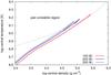 |
Fig. 1 Evolution of central density and temperature of our PISN progenitor models. In the “pair-unstable region”, the stars become dynamically unstable. |
2. Stellar evolution
We follow evolution of stellar structure by using a public stellar evolution code MESAstar version 6208 (Paxton et al. 2011, 2013). We use the hydrodynamic mode of the code throughout this paper. We follow the evolution of three PISN progenitors whose initial masses are 150, 200, and 250 M⊙. The initial metallicity is Z = 0. MESAstar is demonstrated to be able to follow the RSG pulsations that we investigate in this paper (Paxton et al. 2013). An example of input parameters for MESAstar used in this study is shown in Appendix A.
The mixing-length theory is adopted to treat convection using the Schwarzschild criterion. The mixing-length parameter is set as 1.6. Overshooting and semi-convection are not taken into account. We use the “approx21” nuclear network which covers the major important nuclear reactions (Timmes 1999). Although our stars are metal-free at the beginning, the stellar surface metallicity slightly increases as the stars evolve. As a result, the stellar mass is reduced due to the radiation-driven wind, especially during the post-main-sequence. When the stellar effective temperature is higher than 104 K, we use the mass-loss rates formulated by Vink et al. (2001). For the cooler stars, we use the mass-loss rates of de Jager et al. (1988) with the metallicity dependence of Z0.5 (Kudritzki et al. 1987).
The stars are evolved from the pre-main-sequence stage. The calculations are terminated soon after the stellar center starts to contract as a consequence of the pair instability (Fig. 1). We first follow the stellar evolution without taking the effect of the RSG pulsations into account. The stellar properties at the end of these calculations are listed in Table 1 (the ε = 0 models). The evolution of our stars in the Hertzsprung-Russell (HR) diagram is presented in Fig. 2. All the stars evolve into RSGs and explode during the RSG stage as PISNe. The evolutionary tracks of our PISN progenitors are consistent with those obtained in previous studies (e.g., Yoon et al. 2012). The Kippenhahn diagrams for our models are shown in Fig. 3. Our models without mass-loss enhancement have large convective hydrogen-rich envelopes during the late stages when they are RSGs. We investigate the pulsational properties of the stars at the RSG stage in the next section.
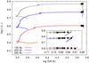 |
Fig. 2 Evolution of our PISN progenitor models in the HR diagram. Those models marked with the symbols are used to examin their pulsational properties. We do not find unstable pulsations in models marked by open circles. The models indicated with squares have the pulsational pattern A, those with triangles have the pattern B, and those with filled squares have the pattern C. See Fig. 4 for the definitions of the patterns. |
3. Pulsations and mass loss
3.1. Pulsation properties
To investigate the pulsational properties of the PISN progenitors during the RSG stage, we use the stellar models that are indicated in Fig. 2. We restart the calculations from these models by forcing the time steps to be less than 0.001 years to follow the pulsations of the stars. The pulsational periods of RSGs were found to be of the order of 1000 days in the previous studies (Heger et al. 1997; Yoon & Cantiello 2010, see also Fig. 5) and we choose small enough time steps to resolve such presumed periods.
We follow the evolution with the small time steps for at least 100 years to check whether pulsations develop and if so, whether the pulsational amplitude grows. The models in which we do not find pulsations with a growing amplitude are indicated with open circles in Fig. 2. These models are either pulsationally stable, or they are unstable but with such a small growth rates that the pulations are damped numerically. In either case, we assume that pulsationally induced mass loss may be neglected in these models.
For the models marked with filled symbols in Fig. 2, we find pulsations with growing amplitudes, as in previous studies of less massive RSGs (e.g., Heger et al. 1997; Yoon & Cantiello 2010). We assume the convective flux to adjust instantly during the pulsations, as Heger et al. (1997); Yoon & Cantiello (2010), even though the convective and the pulsation timescales are comparable. However, note that Heger et al. (1997) found that the pulsational growth rates in their non-linear numerical calculations to be consistent with those computed from linear stability analysis, where the convective flux is assumed to be frozen in. Since Heger et al. (1997) found that two different extreme assumptions on the behavior of the convective flux during the pulsation lead to very similar results, and also Langer (1971) found that the growth rate of the pulsations does not depend on the phase-lag parameter in the simple time-dependent convection model of Arnett (1969), we are confident in the main features of our pulsational analysis. Still, a physically more correct treatment of the coupling between convection and pulsations is desirable, which proves to be difficult to be set up in a parameter-free way (Gastine & Dintrans 2011; Sonoi & Shibahashi 2014).
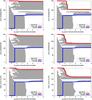 |
Fig. 3 Kippenhahn diagrams for our stellar evolution models. Models in the left column are computed without pulsation-driven mass loss (ε = 0) and those in the right column include pulsation-driven mass loss with ε = 0.1. The initial masses of the models are 150 (top), 200 (middle), and 250 M⊙ (bottom). |
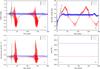 |
Fig. 4 Examples of the pulsations of the PISN progenitors during the RSG stage. Three representative 200 M⊙ models are shown. No pulsation-induced mass-loss enhancement is taken into account in the models of this figure. Evolution of a) relative surface radii; b) total kinetic energy in the star; c) mass-loss rates; and d) total stellar masses is shown. |
We find three different patterns in the way how the amplitudes grow (Fig. 4). In the first pattern named A, the pulsational amplitude grows exponentially at first. Then, the pulsation saturates and the stars continue to pulsate with a constant amplitude. The pulsational amplitudes of the stars with the second pattern B grow exponentially at first but the amplitudes are suddenly damped. Then, the amplitudes start to grow exponentially again until they are damped again. The exponential growth and the sudden damping of the pulsational amplitudes are repeated. The likely reason for the sudden damping is the increase of the radiation-driven mass loss (Fig. 4c). When the pulsational amplitude gets sufficiently large, the radiation-driven mass-loss rates become large because the stars get cooler as they expand. When the amplitude is damped, the mass-loss rates become small again and pulsations can grow again. In the final pattern C, the pulsational amplitudes grow exponentially until the stellar surface reaches the escape velocity. The time steps of our calculations become very small when this happens and we stop the calculations at that moment. The pulsational patterns we obtained for each models are indicated with different symbols in Fig. 2.
In the unstable models, we can find the exponential growth of pulsational amplitudes at least initially in all the patterns. We evaluate the period P and the growth rate η during the initial exponential growth phase for these unstable models. If the exponential growth of the pulsations is proportional to exp(iσt), the growth rate is defined as η ≡ − ℑσ/ ℜσ where ℑσ is the imaginary part of σ and ℜσ is the real part of σ. ℜσ and ℑσ can be estimated from P and the exponential growth of the surface radius, respectively. The periods in our pulsating models are summarized in Fig. 5. The periods of the pulsations in convective stars are expected to follow P ∝ R2/M (Gough et al. 1965) as we find in our models, where R is the stellar radius. The growth rates η are presented in Fig. 6. We find the following strong correlation between η and the effective temperature Teff:  (1)where Teff is in K and the error is the standard error. The obtained relation indicates that the stars with Teff ≲ 4992 K are pulsationally unstable in our models.
3.2. Pulsation-induced mass loss
We have investigated the pulsational properties of the PISN progenitors during their RSG stage. So far, we have not related the pulsations to stellar mass loss. As we introduced in Sect. 1, stellar pulsations may be able to induce mass loss. In this section, we relate the pulsational properties of RSGs to the stellar mass-loss rates. The consequences of pulsation-driven mass loss are investigated in the next section.
We relate the kinetic energy gain of the growing pulsations to mass loss. We assume that a fraction ε of the gained kinetic energy ΔEkin at each time step is used to induce mass loss. We estimate the mass-loss rate Ṁkin induced by the pulsations as  (2)where vesc is the escape velocity from the stellar surface and Δt is the time step (cf. Appenzeller 1970b; Baraffe et al. 2001). In the following stellar evolution calculations, we account of the pulsation-induced mass loss (Eq. (2)) in addition to the radiation-driven mass loss. The kinetic energy does not always increase even if the pulsational amplitude is exponentially growing (cf. Fig. 4b). When ΔEkin< 0, Ṁkin is set to 0.
When Ṁkin> 0, a fraction of the kinetic energy in the star is supposed to initiate mass loss and the corresponding amount of the kinetic energy needs to be reduced from the pulsations. When the star with the kinetic energy Ekin gains ΔEkin, then εΔEkin is supposed to initiate mass loss and the same amount of the kinetic energy in the star needs to be reduced. We reduce the kinetic energy in the stars by reducing the velocities of all the mesh points in the stars as  (3)where vnew and vold are the new and old velocities, respectively. By adopting vnew, the kinetic energy which is supposed to induce mass loss is actually removed from the stellar models.
We obtain Ekin, and thus ΔEkin, by integrating the kinetic energy of all the mass shells in the stars. Then, we reduce the velocities inside the entire star by Eq. (3). However, the pulsating layers gaining the kinetic energy are only located near the surface, as can be seen in the velocity structure of an unstable star presented in Fig. 7. Although we obtain and reduce the kinetic energy in the entire star, only the outer layers which induce the mass loss have an essential effect on the determination of Ekin and the reduction of the velocities.
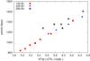 |
Fig. 5 Period P of the pulsations we obtained in our RSGs as a function of R2/M. |
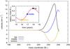 |
Fig. 7 Internal velocity structure of a pulsating model. The velocity structure at three representative times indicated in the inset are shown. The model is obtained from the 250 M⊙ sequence at log Teff/ K = 3.680 and log L/L⊙ = 6.872 with ε = 0. The model is the same as that with ε = 0 presented in Fig. 8. |
3.3. Pulsation-induced mass-loss rates
Using the mass-loss prescription with the kinetic energy reduction explained in the previous section, we perform evolutionary calculations with small time steps (Δt ≤ 0.001 years) as in Sect. 3.1 to investigate the effect of the pulsation-driven mass loss on the evolution of the stars. For this purpose, we select some pulsationally unstable models obtained in Sect. 3.1 and calculate the stellar evolution with ε = 0.1,0.3,0.5, and 0.8.
Figure 8 shows examples of the results with the mass-loss enhancement. All the models presented in Fig. 8 are evolved starting from the 250 M⊙ model with log Teff/ K = 3.680 and log L/L⊙ = 6.872. The model with ε = 0 is the original model without the extra mass loss. The original model has the pulsation pattern C. The models with mass-loss enhancement are indicated with the adopted ε. Since a fraction of the gained kinetic energy is taken out for the mass loss in the new models, their growth rates are smaller than those without the mass-loss enhancement. This can be clearly seen in Fig. 8b where the total stellar kinetic energy of the models is shown. The changes in the growth rates result in changes of the pulsation patterns. While the original model (ε = 0) and the model with ε = 0.1 have the pattern C, the enhanced models with ε = 0.3 and 0.5 show the pattern B. In the ε = 0.8 model, the exponential growth of the pulsational amplitude is terminated early on and the pulsational pattern becomes A. This is because most of the gained kinetic energy is used for the mass loss and the amplitude cannot grow much.
The mass-loss rates of our models are presented in Fig. 8c. The pulsation-driven mass loss is activated only when kinetic energy is gained by the pulsations, making the mass-loss rates strongly time dependent. The resulting mass evolution is shown in Fig. 8d. As the pulsation grows, the mass-loss rates increase due to the increase of the energy gain of the pulsations. A significant amount of mass is lost when the mass-loss rates become large enough. In the cases with ε = 0.3 and 0.5, the large mass ejection results in damping of the pulsation. The pulsation amplitude grows again after the damping and large mass ejections occur intermittently. In the case of ε = 0.8, the amplitude growth stops at early time because a large amount of the gained kinetic energy is used for the mass loss, making the growth less efficient. In this case, the kinetic energy induced mass loss also saturates.
Based on the pulsational calculations with the enhanced mass loss, we estimate the average mass-loss rates of each models. If the pulsational pattern is A, we obtain the average mass-loss rate when the pulsation is saturated. For instance, for the model with ε = 0.8 in Fig. 8, the estimated mass-loss rate is 3 × 10⁻³M⊙ yr-1. For the pattern B, the representative mass-loss rates are obtained based on the mass lost after the first large mass ejection. For example, in the model with ε = 0.3 in Fig. 8, we take the mass just after the large mass ejection at 50 years and we obtain the average mass-loss rate in 50 years, namely, 2 × 10⁻²M⊙ yr-1. For the pattern C, we evaluate the mass difference between the initial and final models and divide it by the time that we could follow the model to obtain the average mass-loss rates. These ways to estimate the average mass-loss rates are not free of arbitrariness and the estimated mass-loss rates can change by a small factor depending on the adopted ways.
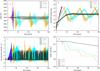 |
Fig. 8 Examples of the evolution of the RSG pulsations in which the mass-loss enhancement by the pulsations is taken into account. A fraction ε of the gained kinetic energy is assumed to be used to induce mass loss. All the models are started from the 250 M⊙ model at log Teff/ K = 3.680 and log L/L⊙ = 6.872. The model with ε = 0 is calculated without mass-loss enhancement. Evolution of a) surface radii; b) total kinetic energy in the star; c) mass-loss rates; and d) total stellar masses is shown. |
The average mass-loss rates we obtained are shown as a function of the growth rate in Fig. 9. The growth rates are those obtained in the models without the mass-loss enhancement (ε = 0). We use the growth rate without the mass-loss enhancement so that we can relate the enhanced mass-loss rates to Teff with Eq. (1), as is applied in the next section. We find that the mass-loss rates with the pulsations generally increase as the growth rates increase. We find substantial mass-loss rates in the models with ε = 0.1,0.3, and 0.5, especially when η is large. For the models with ε = 0.8, the mass-loss rates are not as large as those in other enhanced models. This is presumably because of the large reduction of the pulsational amplitudes due to the large loss of the kinetic energy. Note that for ε = 1, the pulsational mass loss must vanish.
By fitting the mass-loss rates in Fig. 9 with exponential functions, we find the following pulsation-induced mass-loss rates: 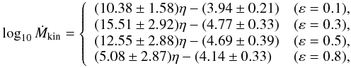 (4)where Ṁkin is in the unit of M⊙ yr-1.
4. Consequences of the mass-loss enhancement
4.1. Stellar evolution
In the previous section, we have selfconsistently evaluated the effect of pulsationally induced mass loss on the pulsations and on the evolution of the stars. However, these calculations are time consuming and hard to be conducted over more than a few hundred pulsation cycles. To investigate the effect of the enhanced mass loss on the entire evolution and final fates of PISN progenitors, we calculate the evolution of the 150, 200, and 250 M⊙ stars with large time steps such that pulsations cannot develop, and we add the pulsation-induced mass-loss rate Ṁkin by applying Eq. (4). The growth rate η is evaluated based on Teff through Eq. (1). When η ≤ 0, we set Ṁkin = 0. We investigate the cases of ε = 0.1 and 0.3.
The results of these calculations are summarized in Table 1. We find that the stellar masses at oxygen core collapse are significantly reduced compared to the models without pulsationally induced mass loss. The mass-loss histories of these models are presented in Fig. 10. The Kippenhahn diagrams for the models with ε = 0.1 are compared with those without mass-loss enhancement in Fig. 3. The mass-loss rates start to be enhanced when hydrogen-rich envelopes become convective and stars enter the RSG stage, as shown in the Kippenhahn diagrams. During the final 103 − 104 years, they are factors of ~10 larger than the radiation driven mass-loss rates, and amount to ~3 × 10⁻⁴M⊙ yr-1.
The large differences in the mass-loss rates may cause drastic changes in the circumstellar environment of PISN progenitors. In most models with the mass-loss enhancement, the CSM density becomes more than one order of magnitude higher. The higher density CSM will affect the observational properties of PISNe, as we discuss in the next section.
The high pulsational mass-loss rates of PISN progenitors do not prevent them from exploding as PISNe. This is because the mass-loss enhancement is caused by the pulsations of the hydrogen-rich envelope after the core hydrogen burning and the mass-loss enhancement will terminate before the entire hydrogen-rich envelope is ejected. At this stage, the stars are not predicted to be pulsationally unstable. Hence, the helium core mass is not reduced as can be clearly seen in the Kippenhahn diagrams in Fig. 3. The pulsational mass loss only results in the significant reduction in the hydrogen-rich envelope mass in PISN progenitors.
Although we focus on the PISN progenitor mass range in this paper, the pulsational amplitude growth is not limited to this mass range. For example, Yoon et al. (2012) show that the non-rotating zero-metallicity stars with initial masses higher than 250 M⊙ also evolve into RSGs. Baraffe et al. (2001) also found that those higher mass stars evolve to RSGs and become pulsationally unstable. Thus, very massive stars can experience large mass loss as RSGs even if they are metal-free. The enhanced mass loss in these very massive stars may lead to dust production in the early Universe even if they do not explode eventually (Nozawa et al. 2014).
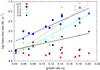 |
Fig. 9 Average mass-loss rates of the stars with the pulsation-induced mass loss. The mass-loss rates depend on the growth rate η. Exponential fits to the estimated mass-loss rates (Eq. (4)) are shown with lines. |
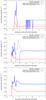 |
Fig. 10 Comparisons of the mass-loss rates between the models with and without the mass-loss enhancement. The mass-loss rates of Eq. (4) with the indicated ε are added in the enhanced models. |
4.2. Metal-free pair-instability supernovae
The high mass-loss rates in PISN progenitors are expected to have significant influence on the observational properties of PISNe. First, the extra mass loss significantly reduces the ejecta mass of PISNe. The hydrogen-rich envelopes of 40 − 70M⊙ are reduced in our models with the mass-loss enhancement compared to those without. The mass of the hydrogen-rich envelopes affect the light-curve properties of PISNe like the duration of the plateau phase (e.g., Kasen et al. 2011).
The mass which is ejected from the PISN progenitors forms their CSM. They can sustain their high mass-loss rates (≳10-4M⊙ yr-1 with ~100 km s-1) until the time of the explosion (Fig. 10). Thus, they are embedded into a dense CSM when they explode. The CSM density can be similar to that estimated in Type IIn SNe (e.g., Kiewe et al. 2012; Taddia et al. 2013; Moriya et al. 2014) and the PISN observational properties are likely to be strongly affected by the dense CSM. For example, our 150 M⊙ PISN progenitor has a 74 M⊙ helium core. It is expected to explode as a PISN, but a small amount of 56Ni (~0.1 M⊙) is expected to be produced by the explosion (Heger & Woosley 2002). Thus, the SN does not get bright by 56Ni heating and it can only be as bright as ≃− 18 mag in the optical due to shock heating (e.g., Kasen et al. 2011; Kozyreva et al. 2014). However, if they have a dense CSM, the interaction between the SN ejecta and the dense CSM can provide an extra heating source to make them brighter. Since the explosion energy of PISNe is very high (~1052 erg, Heger & Woosley 2002), the very energetic SN ejecta clashing into the dense CSM can actually make even 56Ni-poor PISN very bright. The corresponding PISNe can be observed as bright Type IIn SNe with little 56Ni.
The only suggested way to have dense CSM around the very massive stars so far is related to the (core) pulsational pair instability (e.g., Woosley et al. 2007). This mechanism can work in massive stars which are slightly lighter than those which explode as PISNe, and they can lose a large amount of mass by the central pair instability causing a partial ejection of the stellar material. However, the stellar mass range to cause the pulsational pair instability is limited (e.g., Heger et al. 2003; Chatzopoulos & Wheeler 2012a). We find that higher mass stars can also lose a large amount of mass due to (envelope) pulsations. The progenitor mass range for very massive stars exploding within a dense CSM is therefore wider than previously thought.
A critical difference between pulsational pair-instability SNe and PISNe is whether they are actually accompanied by the explosions of the star. Pulsational pair-instability SNe become bright due to the collision of two or more massive shells ejected by the progenitor and they might not be accompanied by actual SN explosions. Conversely, PISNe are actual explosions which destroy the entire star without leaving any remnant. If the mass-loss rates of PISN progenitors are enhanced by the pulsations, actual SN explosions occur within a dense CSM.
High mass-loss rates of PISN progenitors may also end up with the formation of a dense photoionization-confined shell if they are born in an environment with a large ionizing-photon flux like massive star clusters (Mackey et al. 2014). Collision to such massive shell may result in rebrightening of PISN light curves as discussed by Mackey et al. (2014). The confined shells may also make PISNe very bright X-ray and/or radio transients even if they are not dense enough to affect the optical luminosity (e.g., Pan et al. 2013).
Our finding that PISNe may have high mass-loss rates and explode within a dense CSM even if they are metal-free alters our expectation of the observational properties of the first SNe in the Universe. It has long been believed that the first SN progenitors do not suffer much mass loss and the first SNe were considered to explode in a sparse CSM. However, they may actually have a dense CSM environment and not contain massive hydrogen-rich envelopes. Especially, the existence of a dense CSM can make PISNe brighter and bluer than previously expected and they may be easier to find at very high redshifts than previously thought (e.g., Scannapieco et al. 2005; Tanaka et al. 2012, 2013; Pan et al. 2012; Hummel et al. 2012; de Souza et al. 2013). Cooke et al. (2009, 2012) may have already detected this kind of SNe up to z = 3.90. Many PISNe from the first stars can be SLSNe with Type IIn SN spectra and they can be easier to identify. We investigate the detailed observational properties of PISNe exploding within a dense CSM in a forthcoming paper.
4.3. Superluminous supernovae and finite-metallicity pair-instability supernovae
Type IIn SLSNe like SN 2006gy are estimated to have both dense CSM (~0.1 M⊙ yr-1 with 100 km s-1) and very high explosion energy [~(5 − 10) × 1051 erg, e.g., Smith & McCray 2007; Chevalier & Irwin 2011; Ginzburg & Balberg 2012; Moriya et al. 2013; Chatzopoulos et al. 2013; Moriya & Maeda 2014]. Energetic explosions with little 56Ni and a dense CSM are qualitatively expected from our 150 M⊙ models. However, the maximum mass-loss rate we obtained is 2.5 × 10⁻²M⊙ yr-1 (Fig. 9), which is still one order of magnitude lower than those estimated for SLSNe of Type IIn. To obtain mass-loss rates as high as 0.1 M⊙ yr-1, η needs to be 0.24 − 0.28 depending on ε (Fig. 9). The required η and the η-Teff relation (Eq. (1)) indicate that corresponding RSG PISN progenitors have lower effective temperature than Teff ≃ 4600 − 4700 K to have the mass-loss rates higher than 0.1 M⊙ yr-1. Although none of our models have effective temperature as low as 4600 − 4700 K because of the extremely low metallicity, higher-metallicity RSG PISN progenitors can be cooler than 4600 − 4700 K (Langer et al. 2007) and they are therefore likely to have mass-loss rates as high as 0.1 M⊙ yr-1. Thus, they are a strong candidate for the progenitor of Type IIn SLSNe.
Another interesting feature of observed SLSNe is that those that have slowly declining light curves which are consistent with large production of 56Ni are all Type Ic (e.g., Gal-Yam 2012). This indicates that PISNe with massive cores producing a large amount of 56Ni may not explode with their hydrogen-rich envelope. Although none of our models lose all of their hydrogen-rich envelope, the hydrogen-rich envelopes may be removed more easily with the help of the larger radiation-driven mass-loss rates in higher metallicity PISN models (Langer et al. 2007). Thus, the local PISNe may tend to have little or no hydrogen left when they explode because of the pulsational mass-loss enhancement with radiation-driven mass loss, making them primarily Type Ic. If their cores are massive enough to have large 56Ni, they are observed as Type Ic SLSNe with large 56Ni mass. If PISN progenitors with low-mass cores succeed in losing their hydrogen-rich envelopes, they do not produce much 56Ni but they can still be observed as relatively faint Type Ic SNe because of shock heating (Herzig et al. 1990).
Some Type Ic SLSNe have rapidly declining light curves which are not consistent with 56Ni heating (e.g., Quimby et al. 2011; Pastorello et al. 2010; Chomiuk et al. 2011). There are several mechanisms said to explain their high luminosities without 56Ni heating (e.g., Kasen & Bildsten 2010; Dessart et al. 2012; Inserra et al. 2013; Nicholl et al. 2013; Metzger et al. 2014). One possibility is that SLSN progenitors are surrounded by a hydrogen-free dense CSM (e.g., Blinnikov & Sorokina 2010; Leloudas et al. 2012; Moriya & Maeda 2012; Ginzburg & Balberg 2012; Benetti et al. 2014). Pulsational pair-instability SNe from large hydrogen-free cores have been argued to make such a hydrogen-free dense CSM (e.g., Chatzopoulos & Wheeler 2012b, see also Chevalier 2012 for another suggested way). Hydrogen-free cores massive enough to induce pulsational instability SNe may be created by rapidly-rotating stars (e.g., Yoon et al. 2012; Chatzopoulos & Wheeler 2012a, see also Yoon et al. 2006). As discussed previously, we argue that hydrogen-free cores may also come from non-rotating stars with the pulsation-driven mass-loss enhancement. Very massive stars causing pulsational pair-instability SNe also evolve to RSGs (e.g., Yoon et al. 2012; Chatzopoulos & Wheeler 2012a) and they can lose a significant amount of their hydrogen-rich envelope during the RSG stage. The subsequent core pulsational instability may end up with the creation of a massive hydrogen-free CSM which is said to account for rapidly declining Type Ic SLSNe.
5. Conclusions
We have shown that PISN progenitors during the RSG stage are pulsationally unstable. A growing pulsational amplitude may induce mass loss and even metal-free PISN progenitors can have high mass-loss rates.
We find that metal-free PISN progenitors can be pulsationally unstable when their effective temperature is lower than ≃5000 K. The growth rate of the pulsations is found to strongly correlate with Teff (Eq. (1)). If part of the kinetic energy gain of the pulsation is used to initiate mass loss, the mass-loss rate can be very high even if stars are metal-free and the radiation-driven mass loss is inefficient (Eq. (4) and Fig. (9)).
The mass-loss rates of our PISN progenitor models within ~103 years before the explosions become higher than 10-4M⊙ yr-1 when the pulsation-driven mass loss is taken into account (Fig. 10). Because the mass-loss enhancement by the pulsations is initiated in the hydrogen-rich envelope after the hydrogen burning, the mass-loss enhancement stops before the entire hydrogen-rich envelope is lost. Thus, the helium core mass is not reduced by the pulsation-driven mass loss and the stars can still explode as PISNe (Fig. 3).
The pulsation-driven mass loss significantly reduces the masses of PISN progenitors at the time of their explosions (Table 1). Moreover, it forms a dense CSM around PISN progenitors, which can significantly affect the observational properties of the SNe. The existence of a dense CSM around PISNe can make them brighter and bluer, making them easier to observe at high redshifts than previously thought. Our results also show that metal-free very massive stars do not need to be within a limited mass range of pulsational pair-instability SNe to have a dense CSM.
Type IIn SLSNe are estimated to have dense CSM (~0.1 M⊙ yr-1 with 100 km s-1), high explosion energy ~(5 − 10) × 1051 erg, and little 56Ni production. If we account for the pulsation-driven mass loss, these features are expected from low-mass PISN progenitors around 150 M⊙. Although our metal-free PISN progenitors do not become cool enough to make the mass-loss rate as high as ~0.1 M⊙ yr-1, the higher-metallicity PISN progenitors are likely to be cool enough to obtain such high mass-loss rates. PISN candidates with a large 56Ni production found so far are all Type Ic SNe and they do not have hydrogen at all. They may not have hydrogen because the hydrogen-rich envelope is taken away by the pulsation-driven mass loss. Pulsational pair-instability SNe in such hydrogen-free cores may end up with rapidly declining Type Ic SLSNe. Detailed properties of PISNe within a dense CSM from pulsation-driven mass enhancement will be presented in our forthcoming paper.
Acknowledgments
We would like to thank the referee, André Maeder, for constructive comments. T.J.M. is supported by Japan Society for the Promotion of Science Postdoctoral Fellowships for Research Abroad (26·51). Numerical computations were carried out on computers at Center for Computational Astrophysics, National Astronomical Observatory of Japan.
References
- Aoki, W., Tominaga, N., Beers, T. C., Honda, S., & Lee, Y. S. 2014, Science, 345, 912 [NASA ADS] [CrossRef] [PubMed] [Google Scholar]
- Appenzeller, I. 1970a, A&A, 5, 355 [NASA ADS] [Google Scholar]
- Appenzeller, I. 1970b, A&A, 9, 216 [NASA ADS] [Google Scholar]
- Arnett, W. D. 1969, Ap&SS, 5, 180 [NASA ADS] [CrossRef] [Google Scholar]
- Baraffe, I., Heger, A., & Woosley, S. E. 2001, ApJ, 550, 890 [NASA ADS] [CrossRef] [Google Scholar]
- Barkat, Z., Rakavy, G., & Sack, N. 1967, Phys. Rev. Lett., 18, 379 [NASA ADS] [CrossRef] [Google Scholar]
- Benetti, S., Nicholl, M., Cappellaro, E., et al. 2014, MNRAS, 441, 289 [NASA ADS] [CrossRef] [Google Scholar]
- Blinnikov, S. I., & Sorokina, E. I. 2010 [arXiv:1009.4353] [Google Scholar]
- Bowen, G. H. 1988, ApJ, 329, 299 [NASA ADS] [CrossRef] [Google Scholar]
- Chatzopoulos, E., & Wheeler, J. C. 2012a, ApJ, 748, 42 [NASA ADS] [CrossRef] [Google Scholar]
- Chatzopoulos, E., & Wheeler, J. C. 2012b, ApJ, 760, 154 [NASA ADS] [CrossRef] [Google Scholar]
- Chatzopoulos, E., Wheeler, J. C., Vinko, J., Horvath, Z. L., & Nagy, A. 2013, ApJ, 773, 76 [NASA ADS] [CrossRef] [Google Scholar]
- Chen, K.-J., Woosley, S., Heger, A., Almgren, A., & Whalen, D. J. 2014, ApJ, 792, 28 [CrossRef] [Google Scholar]
- Chevalier, R. A. 2012, ApJ, 752, L2 [NASA ADS] [CrossRef] [Google Scholar]
- Chevalier, R. A., & Irwin, C. M. 2011, ApJ, 729, L6 [Google Scholar]
- Chomiuk, L., Chornock, R., Soderberg, A. M., et al. 2011, ApJ, 743, 114 [NASA ADS] [CrossRef] [Google Scholar]
- Cooke, J., Sullivan, M., Barton, E. J., et al. 2009, Nature, 460, 237 [NASA ADS] [CrossRef] [PubMed] [Google Scholar]
- Cooke, J., Sullivan, M., Gal-Yam, A., et al. 2012, Nature, 491, 228 [NASA ADS] [CrossRef] [PubMed] [Google Scholar]
- de Jager, C., Nieuwenhuijzen, H., & van der Hucht, K. A. 1988, A&AS, 72, 259 [NASA ADS] [Google Scholar]
- de Souza, R. S., Ishida, E. E. O., Johnson, J. L., Whalen, D. J., & Mesinger, A. 2013, MNRAS, 436, 1555 [NASA ADS] [CrossRef] [Google Scholar]
- Dessart, L., Hillier, D. J., Waldman, R., Livne, E., & Blondin, S. 2012, MNRAS, 426, L76 [NASA ADS] [CrossRef] [Google Scholar]
- Dessart, L., Waldman, R., Livne, E., Hillier, D. J., & Blondin, S. 2013, MNRAS, 428, 3227 [NASA ADS] [CrossRef] [EDP Sciences] [Google Scholar]
- Gal-Yam, A. 2012, Science, 337, 927 [NASA ADS] [CrossRef] [PubMed] [Google Scholar]
- Gal-Yam, A., Mazzali, P., Ofek, E. O., et al. 2009, Nature, 462, 624 [NASA ADS] [CrossRef] [PubMed] [Google Scholar]
- Gastine, T., & Dintrans, B. 2011, A&A, 530, L7 [NASA ADS] [CrossRef] [EDP Sciences] [Google Scholar]
- Georgy, C. 2012, A&A, 538, L8 [NASA ADS] [CrossRef] [EDP Sciences] [Google Scholar]
- Ginzburg, S., & Balberg, S. 2012, ApJ, 757, 178 [NASA ADS] [CrossRef] [Google Scholar]
- Gough, D. O., Ostriker, J. P., & Stobie, R. S. 1965, ApJ, 142, 1649 [NASA ADS] [CrossRef] [Google Scholar]
- Heger, A., & Woosley, S. E. 2002, ApJ, 567, 532 [NASA ADS] [CrossRef] [Google Scholar]
- Heger, A., Jeannin, L., Langer, N., & Baraffe, I. 1997, A&A, 327, 224 [NASA ADS] [Google Scholar]
- Heger, A., Fryer, C. L., Woosley, S. E., Langer, N., & Hartmann, D. H. 2003, ApJ, 591, 288 [NASA ADS] [CrossRef] [Google Scholar]
- Herzig, K., El Eid, M. F., Fricke, K. J., & Langer, N. 1990, A&A, 233, 462 [NASA ADS] [Google Scholar]
- Hirano, S., Hosokawa, T., Yoshida, N., et al. 2014, ApJ, 781, 60 [NASA ADS] [CrossRef] [Google Scholar]
- Höfner, S. 2008, A&A, 491, L1 [NASA ADS] [CrossRef] [EDP Sciences] [Google Scholar]
- Höfner, S., Gautschy-Loidl, R., Aringer, B., & Jørgensen, U. G. 2003, A&A, 399, 589 [NASA ADS] [CrossRef] [EDP Sciences] [Google Scholar]
- Hummel, J. A., Pawlik, A. H., Milosavljević, M., & Bromm, V. 2012, ApJ, 755, 72 [NASA ADS] [CrossRef] [Google Scholar]
- Inserra, C., Smartt, S. J., Jerkstrand, A., et al. 2013, ApJ, 770, 128 [NASA ADS] [CrossRef] [Google Scholar]
- Kasen, D., & Bildsten, L. 2010, ApJ, 717, 245 [NASA ADS] [CrossRef] [Google Scholar]
- Kasen, D., Woosley, S. E., & Heger, A. 2011, ApJ, 734, 102 [NASA ADS] [CrossRef] [Google Scholar]
- Kiewe, M., Gal-Yam, A., Arcavi, I., et al. 2012, ApJ, 744, 10 [NASA ADS] [CrossRef] [Google Scholar]
- Kozyreva, A., Blinnikov, S., Langer, N., & Yoon, S.-C. 2014, A&A, 565, A70 [NASA ADS] [CrossRef] [EDP Sciences] [Google Scholar]
- Kudritzki, R. P., Pauldrach, A., & Puls, J. 1987, A&A, 173, 293 [NASA ADS] [Google Scholar]
- Langer, G. E. 1971, MNRAS, 155, 199 [NASA ADS] [CrossRef] [Google Scholar]
- Langer, N., Norman, C. A., de Koter, A., et al. 2007, A&A, 475, L19 [NASA ADS] [CrossRef] [EDP Sciences] [Google Scholar]
- Leloudas, G., Chatzopoulos, E., Dilday, B., et al. 2012, A&A, 541, A129 [NASA ADS] [CrossRef] [EDP Sciences] [Google Scholar]
- Li, Y., & Gong, Z. G. 1994, A&A, 289, 449 [NASA ADS] [Google Scholar]
- Mackey, J., Mohamed, S., Gvaramadze, V. V., et al. 2014, Nature, 512, 282 [NASA ADS] [CrossRef] [Google Scholar]
- Metzger, B. D., Vurm, I., Hascoët, R., & Beloborodov, A. M. 2014, MNRAS, 437, 703 [NASA ADS] [CrossRef] [Google Scholar]
- Moriya, T. J., & Maeda, K. 2012, ApJ, 756, L22 [NASA ADS] [CrossRef] [Google Scholar]
- Moriya, T. J., & Maeda, K. 2014, ApJ, 790, L16 [NASA ADS] [CrossRef] [Google Scholar]
- Moriya, T., Tominaga, N., Blinnikov, S. I., Baklanov, P. V., & Sorokina, E. I. 2011, MNRAS, 415, 199 [NASA ADS] [CrossRef] [Google Scholar]
- Moriya, T. J., Blinnikov, S. I., Tominaga, N., et al. 2013, MNRAS, 428, 1020 [NASA ADS] [CrossRef] [Google Scholar]
- Moriya, T. J., Maeda, K., Taddia, F., et al. 2014, MNRAS, 439, 2917 [NASA ADS] [CrossRef] [Google Scholar]
- Neilson, H. R., & Lester, J. B. 2008, ApJ, 684, 569 [NASA ADS] [CrossRef] [Google Scholar]
- Nicholl, M., Smartt, S. J., Jerkstrand, A., et al. 2013, Nature, 502, 346 [NASA ADS] [CrossRef] [Google Scholar]
- Nozawa, T., Yoon, S.-C., Maeda, K., et al. 2014, ApJ, 787, L17 [NASA ADS] [CrossRef] [Google Scholar]
- Ohkubo, T., Nomoto, K., Umeda, H., Yoshida, N., & Tsuruta, S. 2009, ApJ, 706, 1184 [NASA ADS] [CrossRef] [Google Scholar]
- Pan, T., Kasen, D., & Loeb, A. 2012, MNRAS, 422, 2701 [NASA ADS] [CrossRef] [Google Scholar]
- Pan, T., Patnaude, D., & Loeb, A. 2013, MNRAS, 433, 838 [NASA ADS] [CrossRef] [Google Scholar]
- Pastorello, A., Smartt, S. J., Botticella, M. T., et al. 2010, ApJ, 724, L16 [NASA ADS] [CrossRef] [Google Scholar]
- Paxton, B., Bildsten, L., Dotter, A., et al. 2011, ApJS, 192, 3 [Google Scholar]
- Paxton, B., Cantiello, M., Arras, P., et al. 2013, ApJS, 208, 4 [NASA ADS] [CrossRef] [Google Scholar]
- Quimby, R. M., Kulkarni, S. R., Kasliwal, M. M., et al. 2011, Nature, 474, 487 [NASA ADS] [CrossRef] [Google Scholar]
- Rakavy, G., & Shaviv, G. 1967, ApJ, 148, 803 [NASA ADS] [CrossRef] [Google Scholar]
- Scannapieco, E., Madau, P., Woosley, S., Heger, A., & Ferrara, A. 2005, ApJ, 633, 1031 [NASA ADS] [CrossRef] [Google Scholar]
- Smith, N., & McCray, R. 2007, ApJ, 671, L17 [NASA ADS] [CrossRef] [Google Scholar]
- Sonoi, T., & Shibahashi, H. 2014, PASJ, 66, 69 [NASA ADS] [Google Scholar]
- Sonoi, T., & Umeda, H. 2012, MNRAS, 421, L34 [NASA ADS] [CrossRef] [Google Scholar]
- Susa, H., Hasegawa, K., & Tominaga, N. 2014, ApJ, 792, 3 [Google Scholar]
- Taddia, F., Stritzinger, M. D., Sollerman, J., et al. 2013, A&A, 555, A10 [NASA ADS] [CrossRef] [EDP Sciences] [Google Scholar]
- Tanaka, M., Moriya, T. J., Yoshida, N., & Nomoto, K. 2012, MNRAS, 422, 2675 [NASA ADS] [CrossRef] [Google Scholar]
- Tanaka, M., Moriya, T. J., & Yoshida, N. 2013, MNRAS, 435, 2483 [NASA ADS] [CrossRef] [Google Scholar]
- Timmes, F. X. 1999, ApJS, 124, 241 [NASA ADS] [CrossRef] [Google Scholar]
- Umeda, H., & Nomoto, K. 2002, ApJ, 565, 385 [NASA ADS] [CrossRef] [Google Scholar]
- Vink, J. S., de Koter, A., & Lamers, H. J. G. L. M. 2001, A&A, 369, 574 [NASA ADS] [CrossRef] [EDP Sciences] [Google Scholar]
- Whalen, D. J., Even, W., Frey, L. H., et al. 2013, ApJ, 777, 110 [NASA ADS] [CrossRef] [Google Scholar]
- Whalen, D. J., Smidt, J., Even, W., et al. 2014, ApJ, 781, 106 [NASA ADS] [CrossRef] [Google Scholar]
- Wood, P. R. 1979, ApJ, 227, 220 [NASA ADS] [CrossRef] [Google Scholar]
- Woosley, S. E., Blinnikov, S., & Heger, A. 2007, Nature, 450, 390 [NASA ADS] [CrossRef] [PubMed] [Google Scholar]
- Yong, D., Norris, J. E., Bessell, M. S., et al. 2013, ApJ, 762, 26 [NASA ADS] [CrossRef] [Google Scholar]
- Yoon, S.-C., & Cantiello, M. 2010, ApJ, 717, L62 [NASA ADS] [CrossRef] [Google Scholar]
- Yoon, S.-C., Langer, N., & Norman, C. 2006, A&A, 460, 199 [NASA ADS] [CrossRef] [EDP Sciences] [Google Scholar]
- Yoon, S.-C., Dierks, A., & Langer, N. 2012, A&A, 542, A113 [NASA ADS] [CrossRef] [EDP Sciences] [Google Scholar]
- Yoshida, T., Okita, S., & Umeda, H. 2014, MNRAS, 438, 3119 [NASA ADS] [CrossRef] [Google Scholar]
- Yusof, N., Hirschi, R., Meynet, G., et al. 2013, MNRAS, 433, 1114 [NASA ADS] [CrossRef] [Google Scholar]
Appendix A: Input parameters for MESAstar
An example of the input parameters for MESAstar used in this study is shown. Note that the code needs to be modified to incorporate, e.g., the metallicity dependence of the radiation-driven mass-loss rates below Teff = 104 K.
All Tables
All Figures
|
Fig. 1 Evolution of central density and temperature of our PISN progenitor models. In the “pair-unstable region”, the stars become dynamically unstable. |
| In the text | |
|
Fig. 2 Evolution of our PISN progenitor models in the HR diagram. Those models marked with the symbols are used to examin their pulsational properties. We do not find unstable pulsations in models marked by open circles. The models indicated with squares have the pulsational pattern A, those with triangles have the pattern B, and those with filled squares have the pattern C. See Fig. 4 for the definitions of the patterns. |
| In the text | |
|
Fig. 3 Kippenhahn diagrams for our stellar evolution models. Models in the left column are computed without pulsation-driven mass loss (ε = 0) and those in the right column include pulsation-driven mass loss with ε = 0.1. The initial masses of the models are 150 (top), 200 (middle), and 250 M⊙ (bottom). |
| In the text | |
|
Fig. 4 Examples of the pulsations of the PISN progenitors during the RSG stage. Three representative 200 M⊙ models are shown. No pulsation-induced mass-loss enhancement is taken into account in the models of this figure. Evolution of a) relative surface radii; b) total kinetic energy in the star; c) mass-loss rates; and d) total stellar masses is shown. |
| In the text | |
|
Fig. 5 Period P of the pulsations we obtained in our RSGs as a function of R2/M. |
| In the text | |
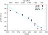 |
Fig. 6 Growth rate η as a function of Teff. The growth rate linearly correlates with Teff (Eq. (1)). |
| In the text | |
|
Fig. 7 Internal velocity structure of a pulsating model. The velocity structure at three representative times indicated in the inset are shown. The model is obtained from the 250 M⊙ sequence at log Teff/ K = 3.680 and log L/L⊙ = 6.872 with ε = 0. The model is the same as that with ε = 0 presented in Fig. 8. |
| In the text | |
|
Fig. 8 Examples of the evolution of the RSG pulsations in which the mass-loss enhancement by the pulsations is taken into account. A fraction ε of the gained kinetic energy is assumed to be used to induce mass loss. All the models are started from the 250 M⊙ model at log Teff/ K = 3.680 and log L/L⊙ = 6.872. The model with ε = 0 is calculated without mass-loss enhancement. Evolution of a) surface radii; b) total kinetic energy in the star; c) mass-loss rates; and d) total stellar masses is shown. |
| In the text | |
|
Fig. 9 Average mass-loss rates of the stars with the pulsation-induced mass loss. The mass-loss rates depend on the growth rate η. Exponential fits to the estimated mass-loss rates (Eq. (4)) are shown with lines. |
| In the text | |
|
Fig. 10 Comparisons of the mass-loss rates between the models with and without the mass-loss enhancement. The mass-loss rates of Eq. (4) with the indicated ε are added in the enhanced models. |
| In the text | |
Current usage metrics show cumulative count of Article Views (full-text article views including HTML views, PDF and ePub downloads, according to the available data) and Abstracts Views on Vision4Press platform.
Data correspond to usage on the plateform after 2015. The current usage metrics is available 48-96 hours after online publication and is updated daily on week days.
Initial download of the metrics may take a while.