| Issue |
A&A
Volume 573, January 2015
|
|
|---|---|---|
| Article Number | A68 | |
| Number of page(s) | 14 | |
| Section | Stellar structure and evolution | |
| DOI | https://doi.org/10.1051/0004-6361/201424589 | |
| Published online | 23 December 2014 | |
Formation of starspots in self-consistent global dynamo models: Polar spots on cool stars⋆
1 Max-Planck-Institut für Sonnensystemforschung, Justus-von-Liebig-Weg 3, 37077 Göttingen, Germany
e-mail: This email address is being protected from spambots. You need JavaScript enabled to view it.
2 Institut für Astrophysik, Georg-August-Universität, Friedrich-Hund-Platz 1, 37077 Göttingen, Germany
Received: 11 July 2014
Accepted: 23 November 2014
Abstract
Context. Observations of cool stars reveal dark spot-like features on their surfaces. These starspots can be more extended than sunspots and cover a large area of the stellar surface. While sunspots appear only at low latitudes, starspots are also found in polar regions, in particular on rapidly rotating stars. Conventional flux-tube models have been invoked to explain starspot properties. However, these models use several simplifications, and so far, neither sunspots nor starspots have been generated in a self-consistent simulation of stellar magnetic convection.
Aims. We aim to clarify the conditions necessary for the spontaneous formation of dark spots in numerical models of convection-driven stellar dynamos.
Methods. We simulated convection and magnetic field generation in rapidly rotating spherical shells assuming anelastic approximation. The high-resolution simulations were performed using a fully spectral magnetohydrodynamic code.
Results. We demonstrate for the first time that a self-consistent distributed dynamo can spontaneously generate high-latitude dark spots. Dark spots are generated when a large-scale magnetic field, generated in the bulk of the convection zone, interacts with and locally quenches flow near the surface. Sufficiently strong density stratification and rapid rotation are prerequisites for the formation of sizeable dark spots in the model.
Conclusions. Our models present an alternative scenario for starspot formation by distributed dynamo action. Our results also lend strong support to the idea that dynamos in the interiors of rapidly rotating stars might be fundamentally different from the solar one.
Key words: starspots / stars: magnetic field / stars: rotation / stars: interiors / dynamo / convection
Two movies are available in electronic form at http://www.aanda.org
© ESO, 2014
1. Introduction
Dark spots are among the most remarkable features on the surface of the Sun. Sunspots are believed to be caused by the interaction of the solar magnetic field with near-surface turbulent convection: in regions of a strong magnetic field, convection is highly quenched, which leads to inefficient transport of heat, which in turn forms local cool and dark spots (see Stein 2012). The size and distribution of regions with a strong magnetic field are ultimately governed by the underlying dynamo mechanism. In the current popular picture of the solar dynamo the interface region of strong radial shear between the radiative core and the convective envelope, the tachocline, is thought to be instrumental (Charbonneau 2005). The tachocline creates a strong toroidal magnetic field by shearing the poloidal field lines. Thin flux-tubes with strong magnetic fields detach from the tachocline and rise to the solar surface where they provide the magnetic field necessary for forming sunspots.
In the past few decades, observational techniques such as photometric light-curve modelling and Doppler imaging (Vogt et al. 1987) have been applied to infer dark starspots on other cool stars. Light-curve modelling is inherently ambiguous1, and gathering good-quality data for Doppler imaging is rather tedious. The evolution of starspots (which appear and disappear during the observations) makes it even more complicated. Nonetheless, there are a few reliable features for which support has been found over the years (see Berdyugina 2005; Strassmeier 2009, and reference therein). A particularly intriguing feature is that starspots occur near the rotational poles of many rapidly rotating stars (Strassmeier 2002). This behaviour is in stark contrast with sunspots, which appear exclusively at low latitudes. Starspots in these stars also appear to be rather large, sometimes covering as much as a few percent of the stellar surface, while the collective area of sunspots even during the solar maximum covers only a small fraction of a percent of the solar photosphere.
By extending the flux-tube models to rapidly rotating cool stars, it has been suggested that rising flux-tubes appear at high latitudes either as a result of the influence of strong Coriolis forces (Schüssler & Solanki 1992; Işik et al. 2011), or that they appear at low latitudes and are then advected polewards by near-surface flows (Schrijver & Title 2001; Holzwarth et al. 2006; Işik et al. 2007, 2011). Mechanism based on magnetic Rossby waves in the tachocline of rapidly rotating stars have also been proposed for polar spot formation (Zaqarashvili et al. 2011).
In contemporary flux-tube models, the formation of dark spots is not considered. These models only provide information about the background magnetic field that supposedly leads to dark spot formation. On the other hand, direct numerical simulations of distributed dynamos and dark spot formation have been rather disconnected. Global dynamo models (e.g. Miesch 2005; Steffen & Freytag 2007; Ghizaru et al. 2010; Käpylä et al. 2012; Gastine et al. 2012; Nelson et al. 2013; Hotta et al. 2014; Fan & Fang 2014) simulate the generation of large-scale magnetic fields, while local simulations (e.g. Vögler et al. 2005; Stein & Nordlund 2006; Rempel et al. 2009; Kitiashvili et al. 2010; Cheung et al. 2010; Stein et al. 2011) study the formation of dark spots in the presence of a prescribed magnetic field. Mitra et al. (2014) recently simulated a self-consistent dynamo using an artificially forced flow in a box-geometry; the resulting magnetic field was able to quench flow in a localized region in the box, mimicking dark spot formation. Although this is certainly a step in the right direction, the setup is simplistic and does not incorporate rotation or convection.
The idea that stellar dynamos necessarily rely on strong shear flow in a tachocline region is certainly worth revisiting, given that flux-tube models are contested even in the solar context (Brandenburg 2005). Furthermore, recent high-resolution numerical simulations of distributed dynamos in spherical shells are also providing a rather different perspective on the solar dynamo (Ghizaru et al. 2010; Käpylä et al. 2012; Nelson et al. 2013). It has been suggested that dynamos in stars in which rotation plays a dominant role might be fundamentally different from the solar case (Christensen et al. 2009; Donati & Landstreet 2009; Reiners 2012). Similar to the dynamos thought to be working in planetary interiors, a distributed dynamo in stars that pervades the entire convection zone can potentially avoid many of the shortcomings of the flux-tube models. For instance, it is hard to imagine how a tachocline region around a geometrically small radiative core in stars (e.g. young pre-main sequence stars or low-mass stars) could govern the dynamo. Flux-tube models that were extended to such stars produced magnetic fields only near the rotational poles (Holzwarth 2004). For fully convective stars the flux-tube picture clearly does not apply. A distributed dynamo, on the other hand, does not need a tachocline and hence can easily operate in stars with small or no radiative cores.
To investigate the generation of a global magnetic field in spherical-shell convection and the simultaneous formation of cool surface spots self-consistently, we further advance a dynamo model that has been applied to gas planets and cool stars (Gastine et al. 2012, 2013a). We do not attempt to model a specific type of star or to match stellar structure and properties as faithfully as possible. Hence this study is in essence exploratory, to find out which basic ingredients are necessary to spontaneously generate dark spots in global numerical simulations without a tachocline. Our main focus is to produce large starspots at high latitudes in the framework of distributed dynamo models.
It is rather tempting to envisage a scenario for polar spots where largely axisymmetric and dipolar magnetic fields, similar in geometry to the fields of Earth or Jupiter, are the backbone. In such dynamos the magnetic field strength naturally peaks at high latitudes. We adopt this as our working hypothesis and pursue it to generate polar spots.
2. Model setup
2.1. Anelastic equations
We used the anelastic magnetohydrodynamic (MHD) equations (Braginsky & Roberts 1995; Lantz & Fan 1999) to simulate the subsonic flows below the photosphere of a star. An electrically conducting fluid convects under the influence of a fixed entropy contrast across a spherical shell with an inner radius ri and outer radius ro. The shell rotates with a constant angular velocity Ω about the z-axis.
The model equations are non-dimensionalised, using the shell thickness d = ro − ri as the reference length scale and the viscous diffusion time d2/ν (ν is viscosity) as the time scale. The density at the outer boundary ρo is used as the density unit and  is the magnetic field scale. The pressure is scaled by ρoνΩ. The magnetic diffusivity λ and the magnetic permeability μ are assumed to be constant. The imposed entropy contrast Δs between the inner and the outer boundary defines the entropy scale.
In the anelastic approximation the thermodynamic variables, density, and pressure, are decomposed into a sum of reference state values and small perturbations as  . The reference state
  corresponds to an adiabatic ideal gas. The reference state density
  and temperature
  are then related by
  , where m is the polytropic index. Assuming a linear variation of gravity, the reference state temperature is given by
 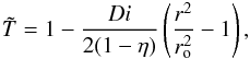 (1)where
 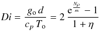 is the dissipation number, go is the gravity at the outer boundary, cp is the specific heat at constant pressure,
 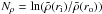 is the number of density scale heights across the shell, and η = ri/ro is the aspect ratio of the spherical shell.
The non-dimensional evolution equation for velocity u is 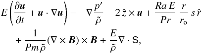 (2)
(2)
where p is the pressure, B is the magnetic field, s is the specific entropy, and  is the radial unit vector.
 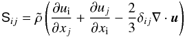 (3)is the traceless rate-of-strain tensor. The entropy is governed by
 ![Mathematical equation: \begin{eqnarray} &&\tilde{\rho}\tilde{T}\left(\frac{\partial s}{\partial t}+{\vec u}\cdot\nabla s\right)\!=\!\frac{1}{Pr}\nabla\cdot(\tilde{\rho}\tilde{T}\nabla s)\nonumber \\ &&\hspace*{5mm} + \frac{Pr\,Di}{Ra}\left[\mathsf{S}^2 + \frac{1}{E\,Pm^2}(\nabla\times{\vec B})^{2}\right]. \label{eq:entropy} \end{eqnarray}](/articles/aa/full_html/2015/01/aa24589-14/aa24589-14-eq33.png) (4)The magnetic field B evolves according to the induction equation
(4)The magnetic field B evolves according to the induction equation 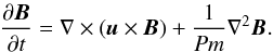 (5)The set of equations is completed by
 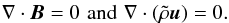 (6)The non-dimensional control parameters appearing in above equations are
 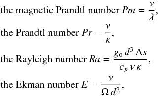 where κ is thermal diffusivity. The transport coefficients ν, λ, κ are assumed constant. To better model magnetic-field-driven structures in outer layers, we used a constant λ. In contrast, earlier studies of stellar dynamos usually assumed a radially increasing λ, making coupling of flow and magnetic field weaker in outer layers (e.g. Browning 2008; Fan & Fang 2014). The aspect ratio η = ri/ro was set to 0.35 for all the simulations reported below.
Following earlier studies (e.g. Fan & Fang 2014), we also report the various energy fluxes that appear in systems governed by the anelastic equations: the entropy diffusion flux Fdiff, the enthalpy flux Fconv, the kinetic energy flux FKE, the viscous diffusion flux Fvisc, the Poynting flux Fpoyn, and the resistive flux Fres. In our non-dimensional units the various fluxes are defined as follows: ![Mathematical equation: \begin{eqnarray} F_{\rm diff}&=&-\frac{1}{Pr}\tilde{\rho}\tilde{T}\left[\nabla s\right]_{r}, \label{eq:flux1} \\ F_{\rm conv}&=&\tilde{\rho}\tilde{T}s\,u_{r}+\frac{Pr\,Di}{E\,Ra}\, P'u_{r}, \\ F_{\rm KE}&=&\frac{Pr\,Di}{Ra}\, u_{r}\left(\frac{\tilde{\rho}u^{2}}{2}\right), \\ F_{\rm visc}&=&-\frac{Pr\,Di}{Ra}\,\left[{\vec u}\cdot \mathsf{S}\right]_{r}, \\ F_{\rm poyn}&=& -\frac{Pr\,Di}{Ra\,E\,Pm}\left[({\vec u}\times{\vec B})\times{\vec B}\right]_{r}, \\ F_{\rm res}&=& \frac{Pr\,Di}{Ra\,E\,Pm^2}\left[(\nabla\times{\vec B})\times{\vec B}\right]_{r}, \label{eq:flux6} \end{eqnarray}](/articles/aa/full_html/2015/01/aa24589-14/aa24589-14-eq44.png) where [...] r represents the radial component.
where [...] r represents the radial component.
2.2. Boundary conditions
Both inner and outer boundaries are impenetrable, stress-free, and electrically insulating. Constant entropy is assumed on both boundaries. Unlike previous numerical studies of stellar convection (Browning et al. 2006; Ghizaru et al. 2010; Käpylä et al. 2010; Masada et al. 2013), we did not model a convectively stable layer below the convection zone. The region below the inner boundary is treated as static.
It is worth noting that our choice of constant entropy on the outer boundary allows the possibility of forming dark spots where heat flux is lower than in neighbouring regions. This was not possible in earlier studies of stellar convection zones where constant heat flux boundary conditions were employed.
2.3. Initial conditions
Global dynamo simulations (Simitev & Busse 2009; Sasaki et al. 2011; Schrinner et al. 2012; Gastine et al. 2013a, 2012; Yadav et al. 2013a) in spherical shells with free-slip boundaries show bistability. In the bistable regime, dynamos that started with a weak and small-scaled magnetic field saturate at a multipolar and non-axisymmetric magnetic field, while the dynamos that started with a magnetic field that had a strong axial dipole saturate in a dipole-dominant field configuration. We used either of these magnetic field configurations as an initial condition to explore different dynamo solutions for a given set of control parameters.
2.4. Numerical technique
The model equations are solved using the MHD-code MagIC (Wicht 2002; Gastine & Wicht 2012), which has been tested using community-based benchmark simulations (Jones et al. 2011). After decomposing the mass flux and magnetic field into toroidal and poloidal components as  the scalar potentials W,X,Y,Z, the pressure, and the entropy are then expressed in terms of spherical harmonics in longitude and latitude and Chebyshev polynomials in radius. The system of equations is time-advanced using an explicit second-order Adams-Bashforth scheme for Coriolis and non-linear terms and an implicit Cranck-Nicolson scheme for the remaining terms (Glatzmaier 1984; Christensen & Wicht 2007).
2.5. Control parameters
Capturing the dynamics of rotationally dominated large-scale convection in stellar interiors is the primary aim of this study, and the control parameters we chose reflect this to some extent. However, the technical feasibility severely constrains our control parameter choice. Hence, this study, or any global numerical study, for that matter, implicitly assumes that the unresolved small-scale turbulence does not affect the large-scale properties of the system. The control parameters for different setups are listed in Table 1.
Simulation setups.
There have been some unsuccessful attempts at generating an axial-dipole dominated (ADD) magnetic field in global numerical simulations with density-stratified convection zones (Dobler et al. 2006; Browning 2008). This is in stark contrast with the studies of planetary dynamos (which usually ignore density stratification), where ADD solutions are found frequently (Jones 2011). The planetary dynamo simulations (e.g. Christensen & Aubert 2006) persistently show that as the Ekman number, which quantifies the importance of viscous effects as compared to rotational effects, is decreased (i.e. increasing rotational influence), ADD magnetic fields become more stable and can be obtained at low values of Pm. For example, ADD fields have been found at Pm as low as 0.06 for E ≈ 10-6 in geodynamo simulations (Christensen & Aubert 2006). Reaching such a small E in anelastic simulations would be a much more demanding task.
Systematic investigations have revealed that as the density stratification increases in the convection zone, ADD dynamos gradually become unstable (Gastine et al. 2012; Schrinner et al. 2014). Schrinner et al. (2014) showed that for moderate Ekman numbers used in density-stratified simulations a high Pm might be favourable for attaining ADD dynamos. Decreasing the amplitude of differential rotation (in the form of prograde equatorial jets that are typically found in simulations) might also help to stabilize ADD dynamos (Duarte et al. 2013; Schrinner et al. 2014). The Prandtl number has been shown to affect the amplitude of the equatorial differential rotation (Christensen 2002; Simitev & Busse 2005). Keeping these results in mind, we used relatively high values of Pr and Pm in our simulations (see Table 1). Moreover, simulations with Pr of 10 generate convection with moderate Reynolds numbers Re = vd/ν (v is some appropriately averaged velocity). Consequently, a relatively high value of Pm is required in these simulations to attain a high enough magnetic Reynolds number Rm = RePm for dynamo action to occur. The Ekman number is set to 3 × 10⁻⁴ (except for S-Pr1-N5). This is equivalent to a Taylor number (=4 /E2) of about 4 × 10⁹. This value allowed us to carry out a small parameter study in a manageable time frame while still having rotationally dominated convection in a medium with strong density stratification.
Simulations with density-stratified convection zones have relatively slower and large-scaled flow in high-density regions while the flow is rapid and has smaller scales in regions of low density. The latter demands smaller time-steps and higher grid resolution. Furthermore, to ensure that a dynamo solution is in an equilibrium state, the simulation should run for at least a magnetic diffusion time, implying a longer run time at higher Pm. Within these constraints, the highest density contrast we could afford in simulations with Pm = 10 was about 150. The polytropic index also had to be increased to 2 (from a more appropriate value of 1.5 for a monoatomic ideal gas) in these cases to avoid a steep drop in density in the outer layers, which would require a higher grid resolution to resolve. For a case with Pm = 2, however, we were able to reach a density contrast of about 400 with a polytropic index of 1.5. An exception was made for model S-Pr1-N5, which was run for a third of the magnetic diffusion time because of the severe computational requirements.
2.6. Numerical grid resolution
All the simulations reported in this study were first run on a grid with 768 × 384 × 121 grid points, where the three numbers represent the grid resolution in longitude, latitude, and radius, respectively. This grid was sufficient to adequately resolve the flow and magnetic field in most of the interior of the shell, but the relatively vigorous convection near the surface remained under-resolved in most cases. We then stepwise increased the grid resolution and ran the simulation long enough to confirm the results. The resolution reported in Table 1 is the highest resolution used for a particular simulation.
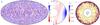 |
Fig. 1 Flow patterns for hydrodynamical model H-Pr10-N5. Hammer projection of radial velocity ur at r = 0.99 ro is displayed in a), while the longitudinally averaged azimuthal velocity ⟨ uφ ⟩ φ (or differential rotation) is given in b). Red and blue indicate a downwelling and an upwelling flow in a) and a westward and an eastward flow in b). ur and ⟨ uφ ⟩ φ are given in terms of the Reynolds number Re = u d/ν and the Rossby number Ro = u/ (dΩ) . The z component of vorticity is shown in c), where red and blue shades represent positive and negative vorticity. The colour variations are saturated at values lower than the extrema. |
3. Results
We begin by discussing the results of a simulation for purely hydrodynamical convection and later explore its dynamo action.
3.1. Hydrodynamical convection
To roughly assess how rapid rotation influences convection, we used the so-called convective Rossby number  (introduced by Gilman 1977), which estimates the ratio of buoyancy to Coriolis forces. For Roc ≪ 1, rotational effects dominate. The model H-Pr10-N5 (see Table 1) has Roc ≈ 0.5. This means that here convection is probably substantially influenced by rotation. Note that Roc can be decreased either by decreasing E (computationally very demanding) or by increasing Pr. The last scenario has been exploited in setting the control parameters for this and most other cases.
Various quantities describing the convection patterns of model H-Pr10-N5 are portrayed in Fig. 1. The radial velocity ur near the outer boundary shown in (a) highlights the typical broad upwellings and narrow downwellings that are formed by the influence of density stratification. The flow in the deep interior, however, consists of large-scale helical columns aligned with the rotation axis, as seen in a 3D rendering (not shown for this case). This convection pattern is typical for rotationally dominated convection in simulations of density-stratified convection zones (Miesch 2005; Browning 2008; Gastine & Wicht 2012). The structural change arises because the influence of rotation varies as a function of radius in a density-stratified fluid and is weaker in the outer layers (Gastine & Wicht 2012). In (b) the axisymmetric longitudinal velocity ⟨ uφ ⟩ φ (angle brackets ⟨ ... ⟩ x represents averaging over x) or the differential rotation varies only moderately on cylinders aligned with the rotation axis, except near the outer boundary. The typical differential rotation profile, that is, faster equator and slower poles, is maintained by the Reynolds stresses, which arise because of the statistical correlation between radial and longitudinal flow components (Christensen 2002; Simitev & Busse 2005). Reynolds stresses are promoted by the spiralling nature of convection columns that are tilted in the direction of the shell rotation (Gilman 1975; Busse 1983). The plot of the axial fluid vorticity ωz = (∇ × u)z in the equatorial plane of the shell in (c) shows the spiralling columns.
A more refined estimate for the rotational influence can be obtained via the local Rossby number (Christensen & Aubert 2006), defined here as a function of radius by Rol = ⟨ u ⟩ θ,φ,t/ (Ωl) with the longitudinally, latitudinally, and time-averaged velocity ⟨ u ⟩ θ,φ,t. The length scale  is a characteristic length scale of the flow at radius r defined using
 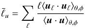 (13)where uℓ is the flow component at a given radius for spherical harmonic degree ℓ. The radial variation of Rol for model H-Pr10-N5 is shown in Fig. 2. Previous parameter studies have shown that as long as Rol is smaller than a threshold value of ≈0.1, Coriolis forces significantly affect the nature of convection (Christensen & Aubert 2006; Schrinner et al. 2012; Gastine et al. 2013b, 2014). Here, Rol< 0.1 in the entire shell. This explains why Fig. 1a shows north-south aligned convection cells even near the outer boundary of the simulation.
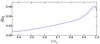 |
Fig. 2 Variation of the local Rossby number Rol as a function of radius for the hydrodynamical model H-Pr10-N5. u and l have been averaged over a few rotation periods. |
3.2. Self-consistent dynamos
3.2.1. Model NA-Pr10-N5
We now consider the dynamo action of the case discussed above. We used the hydrodynamic model H-Pr10-N5 as starting point and set Pm = 10, which results in model NA-Pr10-N5. A very weak seed magnetic field was exponentially enhanced by the helical convection, and the system finally saturated to a statistically stationary state. A snapshot of the simulation in the saturated regime showing the radial velocity and the radial magnetic field near the outer boundary is shown in Figs. 3a and c. The dynamo-generated magnetic field is non-axisymmetric, and the morphology is dominated by a spherical harmonic order m = 1 component. The magnetic field at the instant shown in Fig. 3c is also concentrated in the southern hemisphere. However, the hemisphere with the dominant magnetic field can change with time (Grote & Busse 2000). The field also propagates westwards in the rotating frame of reference of the shell. A butterfly diagram (not shown) of the azimuthally averaged radial field also shows poleward-propagating features. Such travelling non-axisymmetric dynamo solutions have previously been observed in dynamos with free-slip boundary conditions (Schrinner et al. 2011, 2012; Käpylä et al. 2013) and can be described in terms of the classical Parker-waves (Busse & Simitev 2006; Goudard & Dormy 2008; Schrinner et al. 2012).
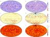 |
Fig. 3 Radial velocity ur at r = 0.99 ro in a), b), radial magnetic field Br at r = 0.99 ro in c), d), and total heat flux F normalized by its surface mean Fmean on the outer surface in e), f) for models NA-Pr10-N5 and A-Pr10-N5. ur is given in terms of the Reynolds number, and the radial magnetic field is normalized by the equipartition field strength calculated using the time-averaged total kinetic energy in the shell. The colour variations for ur and Br are saturated at values lower than the extrema; the full variation range for Br is ≈ ± 0.3 in d). |
As shown in Fig. 3c, the diverging upwellings sweep the magnetic flux and concentrate it into the convergent downwellings. This sort of redistribution of magnetic flux is a generic trait in magnetic convection (Proctor & Weiss 1982; Vögler et al. 2005; Stein & Nordlund 2006; Stein 2012). Furthermore, the expelled magnetic flux preferably accumulates into the nodes of the downwelling lanes of convection cells (Stein 2012).
In Fig. 3e we plot the total heat flux normalized by its surface-averaged value on the outer boundary of the simulation. The heat flux at the outer boundary is calculated as 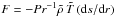 , where and are the local (background) density and temperature and ds/dr is the local radial derivative of entropy. Comparing Fig. 3a with Fig. 1a shows that the radial flow is very similar in both cases. Nonetheless, a careful inspection of the nodes of the downwelling lanes does show a quenching of radial flow where the magnetic flux is concentrated. Correspondingly, the convective heat flux is also reduced in these regions (e.g. the tiny magnetic flux patch near the south pole in Fig. 3c).
Compared with model H-Pr10-N5, the differential rotation (Fig. 4a) is quenched and the eastward tilt of helical convection columns (Fig. 4b) is reduced by the magnetic field in this case. The energy content of the axisymmetric differential rotation for H-Pr10-N5 and NA-Pr10-N5 is about 18% and 8% of the total kinetic energy (Table 1). The qualitative structure of differential rotation, however, is similar in both cases (see Fig. 1b) and Fig. 4a). The total magnetic energy of model NA-Pr10-N5 is only about 30% of the total kinetic energy (see Table 1 and Fig. 5a). In the mean-field formulation, such non-axisymmetric multipolar dynamos can be categorized as αΩ or α2Ω type (Schrinner et al. 2012; Gastine et al. 2012), where magnetic field co-exists with substantial differential rotation. Dynamo simulations resembling this case (i.e. cases with significant density stratification and a multipolar magnetic field) have been reported frequently (Miesch 2005; Browning 2008; Ghizaru et al. 2010; Käpylä et al. 2012; Gastine et al. 2012; Schrinner et al. 2012; Nelson et al. 2013; Fan & Fang 2014; Cole et al. 2014) and do not exhibit any prominent low heat flux regions linked to strong magnetic fields that could be associated with starspots (see Fig. 3e).
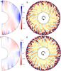 |
Fig. 4 Longitudinally averaged azimuthal flow in a) and c) and ωz in b) and d) for model NA-Pr10-N5 and A-Pr10-N5. |
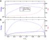 |
Fig. 5 Longitudinally and latitudinally averaged kinetic energy and magnetic energy density on the left axis and magnetic Reynolds number Rm = u d/λ on the right axis as a function of radius for model NA-Pr10-N5 (panel a)) and A-Pr10-N5 (panel b)). The quantities were averaged over a few rotation periods. |
3.2.2. Model A-Pr10-N5: Polar starspots
Instead of initiating the dynamo simulation with a tiny seed magnetic field, we now took the flow input from model H-Pr10-N5 and initiated the dynamo simulation with a strong dipolar magnetic field aligned with the rotation axis. The resulting dynamo model is A-Pr10-N5 (Table 1). The motivation behind starting with a strong dipolar field is to have strong Lorentz forces that can quench the shearing differential-rotation via Maxwell stresses (Ferraro 1937; Aubert 2005). This allows an axial-dipole dominant (ADD) solution to develop and stabilize. As shown in Fig. 4c, the axisymmetric differential rotation becomes even more strongly quenched (energy content of about 3% of the total kinetic energy) compared with the non-magnetic model than for NA-Pr10-N5 and and has entirely lost any semblance to geostrophy. Reynolds stresses are not effective any more because the spiralling of convection columns nearly vanishes (Fig. 4d). Such a differential rotation profile is typically associated with a thermal wind balance (Aubert 2005), that is, a balance of buoyancy and Coriolis forces. This ADD solution is stable because we ran this simulation for about two magnetic diffusion times (d2/λ). This ADD configuration would have decayed after a magnetic diffusion time if it had not been self-consistently sustained by the convection. Note that one magnetic diffusion time is equal to one thermal diffusion time (d2/κ) since both Pm and Pr are equal for this case. Therefore, the simulation is also thermally relaxed.
Dynamos with an ADD magnetic field that co-exist with highly quenched differential rotation are classified as α2-dynamos (Olson et al. 1999; Chabrier & Küker 2006; Schrinner et al. 2012). Dynamos in this state are said to be in a magnetostrophic state where Lorentz forces are rather strong and enter in the first-order force balance (e.g. Sreenivasan & Jones 2006). Generally, parameter studies (Browning 2008; Gastine et al. 2012; Yadav et al. 2013a) show that large-scale magnetic fields generated by a distributed dynamo quench the differential rotation to low values (much lower than solar). Recently, this was empirically verified for a large sample of cool stars that showed a rough inverse correlation between rotation rate and differential rotation (Reinhold et al. 2013). Note that higher rotation rates generally imply stronger magnetic fields in cool stars (Pizzolato et al. 2003).
Figure 6 displays the radial profile of the non-dimensional luminosity L calculated using the various energy fluxes defined by Eqs. ((7)–(12)). The total luminosity Ltot is nearly constant throughout the convection zone, signifying the statistically stationary nature of the solution. Conductive and convective contributions dominate the energy transport, with the former dominating near the boundaries, the latter in the bulk. Assuming that the thermal boundary layers (or better: entropy boundary layers, since entropy diffusion is assumed in our formulation) extend up to the point where diffusive and convective flux contributions are equal (see e.g. Julien et al. 2012), the bottom and top boundary layers span about 0.04 ro and 0.01 ro. The thickness difference between these two boundary layers can be attributed to the high density contrast in the simulated convection zone. Viscous, Poynting, and resistive fluxes are only secondary contributions, similar to what is usually observed in such global convection simulations. Owing to the relatively small role of inertia in this dynamo model (since Pr = 10), the kinetic energy flux also contributes less than in earlier studies, which frequently employed Pr ≤ 1 (e.g. Miesch 2005; Nelson et al. 2013; Fan & Fang 2014).
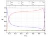 |
Fig. 6 Radial profiles of non-dimensional luminosities, i.e. r2∫ ⟨ F ⟩ tsin(θ) dθ dφ, associated with the different fluxes for model A-Pr10-N5, with Ltot being the sum of all contributions. The different contributions are normalized by Ltot at r = ro. The profiles were averaged for about 200 rotations. |
A snapshot of the radial velocity and the radial magnetic field near the outer boundary is given in Fig. 3b and d. Unlike the multipolar dynamo model NA-Pr10-N5, the quenching of near-surface flows in regions of strong magnetic field is rather prominent in this case and is clearly visible in Fig. 3b, especially at high latitudes. The patch near the north pole with very weak radial flow is larger than the general length scale of the convection cells. At low latitudes convection forms irregular north-south aligned lanes that are associated with narrow elongated flux concentrations that are relatively short-lived. Here the field concentration is usually not strong enough to seriously impede radial flow. We use the term dark spot for a region of substantial size (similar to or larger than the local convection cells) on the surface of the model where the heat flux has been suppressed by at least ≈50% below the average surface heat flux. Because locally very strong magnetic fields severely quench the flow, the convective heat transport is reduced, which leads to the formation of dark spots that can be associated with cool starspots.
A comparison of the radial variation of the kinetic and magnetic energy of model A-Pr10-N5 (Fig. 5b) with that of NA-Pr10-N5 (Fig. 5a) reveals that the magnetic energy dominates in the entire convection zone (on average) in the case with dipolar magnetic field, i.e. this case generates a super-equipartition magnetic field. Note that the production of super-equipartition fields is not novel, and geodynamo simulations frequently produce such strong magnetic fields, mimicking the scenario on Earth where magnetic energy is thought to be much higher than the kinetic energy (by a factor of about 7000; Roberts & Glatzmaier 2000). In the stellar context, Featherstone et al. (2009) have reported a spherical shell dynamo with super-equipartition field strengths. Systematic numerical studies have shown that dipolar dynamos in general produce higher field strengths than the multipolar ones (Christensen 2010; Schrinner et al. 2012; Gastine et al. 2012; Yadav et al. 2013a,b).
The quenching of convective flow that leads to the formation of dark spots in this simulation is a relatively shallow phenomenon. For instance, the flow suppression at the instant shown in Fig. 3 is noticeable down to a depth of about 0.95 ro. However, although shallow, the quenching of convection extends well beyond the outer thermal boundary layer, which reaches down to about 0.99 ro. Figure 7 shows the radial velocity and the radial magnetic field on a cut along the rotation axis at a longitude passing through the large northern spot in Fig. 3d. As is typical in ADD dynamos, a high concentration of magnetic flux exists at high latitudes. The magnetic field associated with this spot is seated in great depth. The integrity of this prominent flux-concentration seems to be maintained by rapid convective downwellings that surround it at its lateral margins (Fig. 7a).
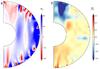 |
Fig. 7 Radial velocity in a) and radial magnetic field in b) on a constant longitude passing through the large polar spot for model A-Pr10-N5. The colour scales saturate at values lower than the extrema. |
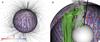 |
Fig. 8 Perspective view of model A-Pr10-N5 (polar spot case) from a northern latitude. a) radial velocity near the outer boundary and the magnetic field lines above the shell, upward continued by assuming a potential field. In b) the surface showing the radial flow in a) is cut and only the eastern hemisphere in shown to visualize the interior magnetic field lines associated with the northern large dark spot (visible as a white patch in a)). The isosurface of the axial vorticity ωz (in green, shown in a limited domain for clarity) is also illustrated in b). |
3.2.3. Time evolution of darkspots
Movie 1 shows the rich dynamics of the radial magnetic field on the outer boundary of model A-Pr10-N5. The units in the movie are similar to Fig. 3f, and it spans about 75 rotations. It shows a prominent high-latitude flux-concentration that evolves on a much longer time scale than the local convection. Large flux-patches remain for many rotations and form when two or more sizeable patches merge. The elongated north-south-aligned convection cells near the equator act as clear pathways for tiny flux patches to migrate latitudinally.
Figure 9 provides a long-term perspective on the simulation by displaying azimuthally averaged radial magnetic field and relative heat flux as a function of time. Generally, the magnetic field shown in (a) is dominated by an ADD configuration. However, the dynamo solution also portrays long-term dynamics where the hemisphere with the stronger magnetic flux switches from one to the other as the simulations progresses (for instance, at around 9000 rotations). The change in the magnetic flux of a hemisphere is clearly visible in (b), which highlights the evolution of the darkest regions on the outer boundary of the simulation. Here the hemisphere with darker spots also switches from the southern to the northern hemisphere. Although low-latitude regions do have small magnetic-field-induced spots, the azimuthal averaging filters them out, which explains the absence of any feature at low latitudes.
In Fig. 8, we show a 3D rendering of model A-Pr10-N5. Figure 8a clearly shows the large-scale component of the magnetic fields, which is dominated by an axial dipole. Figure 8b shows that the field lines in the northern dark spot are rooted in deeper convection columns. Based on Fig. 8b, we can conjecture the following formation mechanism for sizeable dark spots: first, helical columnar convection in the interior generates a collection of twisted and mainly radial magnetic field lines, and, second, the integrity of this stable magnetic structure is maintained by the downwellings of the convection in outer layers at its edges (see also Fig. 7). Since deep-rooted columns are wider and have a longer evolution time scale (sluggish velocity due to higher density), the flux bundles associated with them would appear as a rigid structure to near-surface convection. The dark spots formed as a result of these anchored flux bundles evolve on a time scale longer than local convection.
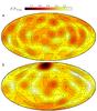
Observational techniques for starspot detection, such as Doppler imaging, provide only a smeared-out picture of the stellar surface. This causes the information about small scale features to be washed out. The high-latitude dark spots are commonly assumed to be a collection of smaller dark spots (Berdyugina 2005; Strassmeier 2009). To better compare our simulation results with the observational Doppler images, we smeared out the details in the simulations by filtering out all spherical harmonic degrees beyond 10 from the original simulation data. The resulting heat-flux fluctuation maps are shown in Fig. 10. In the non-dipolar case NA-Pr10-N5 shown in (a), the fluctuations are moderate and no consistent pattern exists. In the ADD case A-Pr10-N5 shown in (b), the dark spot in the polar region has become even more prominent. Figure 10 also shows other low-contrast features on the surface that do not represent magnetic-field-driven dark spots. Movie 2 shows the time evolution of low-order heat-flux fluctuations corresponding to movie 1. The polar spots in the north pole region maintain a broad dark feature that persists throughout the movie. Other low-contrast features in the movie near the equator and near the south pole are more dynamic.
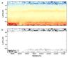 |
Fig. 9 Panel a) shows the azimuthally averaged radial magnetic field on the outer boundary of model A-Pr10-N5 (colour map similar to Fig. 3d). Panel b) highlights magnetic-field-induced dark regions on the outer boundary. The latter were constructed by calculating the azimuthally averaged relative heat flux (sampled in Fig. 3f) for the simulation and plotting data that were lower than unity. |
3.2.4. Synthetic light curves
Synthetic light curves for the simulation with polar spots (model A-Pr10-N5) and the non-magnetic reference model H-Pr10-N5 are shown in Fig. 11. We calculated the light curves for one full rotation following the instance in time at which the flux is shown in Fig. 3. To generate the light curves, the flux at different locations was integrated for the visible hemisphere for different phase angles of rotation. Limb-darkening was incorporated by modulating the visible flux as f(q) = fo (1 − w(1 − cos(q))), where w is a limb-darkening coefficient (set to a nominal value of 0.3), f(q) is the flux observed by the observer, fo is the heat flux at a location on the outer boundary of the simulation, q is the angle between the radius vector to a surface point and the line of sight. The light-curve variations are qualitatively similar for different assumed inclinations of the equatorial plane with respect to the line of sight (pearled curves), however, the amplitude increases for equatorial and northern inclinations. We also calculated the light curves for the hydrodynamic simulation H-Pr10-N5; they are shown using dashed curves. These hydrodynamic light curves show a variation of little more than 1%. The light-curve amplitudes for the hydrodynamic model are similar to the amplitude of the southern inclination light curve of the dynamo case where the large dark spot is not visible. Hence, if we assume that the model inherently produces light-curve modulations of about 1%, the large dark spot near the north pole adds an extra modulation of about 0.5%. Light-curve variations of the order of a few percent are consistent with the observation of active cool stars in the Kepler data set (Basri et al. 2013).
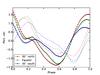 |
Fig. 11 Synthetic light curves calculated using the heat flux emanating from the outer boundary of a simulation. Pearled curves depict model A-Pr10-N5, dashed curves the hydrodynamic model H-Pr10-N5. Light-curves are given for three different inclinations: line of sight 30° north of the equator (red), in the equatorial plane (green), and 30° south of the equator (blue). The amplitude is in terms of percentage variations about the mean. |
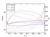 |
Fig. 12 Kinetic energy Ekin (solid curves), magnetic energy Emag (dashed curves), density on the left axis, and magnetic Reynolds number (dotted curves) on the right axis as a function of radius for three models with dipole-dominant magnetic fields, but different density stratification Nρ in the convection zone. Blue, red, and black curves are for models A-Pr10-N3, A-Pr10-N4, and A-Pr10-N5, respectively. |
3.2.5. Importance of density stratification and rotation
The results discussed above demonstrate that for a fixed density stratification and rotation rate multipolar dynamos (generating weaker field strengths) do not produce dark spots, while the ADD dynamos with stronger fields do form dark spots. Using a small parameter study, we now explore the sensitivity of dark spot formation to the density stratification in the convection zone and the rotation rate of the spherical shell.
We simulated two cases with a lower density stratification: model A-Pr10-N4 with Nρ = 4 (density contrast of 55) and model A-Pr10-N3 with Nρ = 3 (density contrast of 20). The entropy contrast (or equivalently Ra) across the shell was changed as well, such that the simulations produced an ADD magnetic field (see Table 1). The resulting radial variation of kinetic and magnetic energy is shown in Fig. 12. As the density stratification is decreased, the magnetic energy near the outer boundary decreases sharply. Figure 13 displays the same quantities as Fig. 3 for model A-Pr10-N3. At a few inter-cellular nodes where the flux is strong enough to locally quench the flow, small dark patches are formed, but the surface is devoid of sizeable dark spots. This suggests that including a high density contrast (Nρ ≥ 5) in the convection zone is instrumental for generating large and persistent dark spots. However, the mechanism through which density stratification promotes larger flux-concentrations is not yet clear. The proposed “negative effective magnetic pressure instability (NEMPI)” (Rogachevskii & Kleeorin 2007; Brandenburg et al. 2011) also highlights the importance of density stratification for generating sizeable magnetic flux concentration. A more detailed analysis is needed to establish a connection between our simulations and the NEMPI mechanism.
Guided by the results of this discussion, we now increased the density contrast to Nρ = 6 (density contrast ≈400; model NA-Pr1-N6) in the convection zone to explore whether a multipolar dynamo can form dark spots as well. Pr and Pm for NA-Pr1-N6 were lowered to avoid long saturation time scales; this came at the expense that a dominantly dipolar magnetic field could not be sustained, however (see Table 1). A snapshot, similar to Fig. 3, of dynamo model NA-Pr1-N6 is shown in Fig. 14. The magnetic field is dominated by a non-axisymmetric m = 1 pattern, and it peaks in two broad longitudes in both hemispheres. This large-scale magnetic field also slowly propagates westwards, similar to model NA-Pr10-N5. The convection near the outer boundary is dominated by small convection cells, not only at high latitudes, as for A-Pr10-N5, but also near the equator. This is due to the higher Rol in this case, which varies from 0.05 in the interior to a maximum of about 0.25 in the outer layers.
Figure 14a and b shows that radial velocity is quenched in many localized regions. This gives rise to dark spots that are smaller than the large spot seen in model A-Pr10-N5, but are still quite sizeable, that is, have the same scale as the convection cells. The light curve of this case, portrayed in Fig. 15, shows double dips that might be associated with the non-axisymmetric heat flux pattern induced by the m = 1 magnetic field geometry. Note that the light-curve amplitudes in this case are significantly smaller than in Fig. 11 because the convection transports only about 30% of total heat in this case compared with about two-thirds in model A-Pr10-N5. Hence, the dark spots in this case have a lower contrast with the regions where the convection operates normally. Cole et al. (2014) have already reported similar westward-drifting magnetic fields in direct numerical simulations. Such dynamo solutions provide a rather enticing explanation for the active-longitudes phenomenon: starspots concentrated in broad preferred longitudes. Cole et al. (2014) have discussed this connection, although their simulation did not generate any dark spots. Our model NA-Pr1-N6 can be considered as a further step in this line of thought since it produces the appropriate magnetic field as well as dark spots.
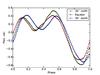 |
Fig. 15 Similar to Fig. 11, but for model NA-Pr1-N6. Light curves are based on the instant shown in Fig. 14. |
The plot in Fig. 16 shows the radial variation of kinetic and magnetic energy density for model NA-Pr1-N6. This model is qualitatively similar to model NA-Pr10-N5 (see Fig. 5a) in that the kinetic energy dominates in this case as well. However, in outer layers, the dominance of kinetic energy is somewhat waker: the ratio of magnetic to kinetic energy density for models NA-Pr10-N5 and NA-Pr1-N6 are 0.18 and 0.25, respectively, about 40% higher in the latter. One might speculate that the higher density stratification and weaker dominance of kinetic energy might explain why model NA-Pr1-N6 generates sizeable dark spots while model NA-Pr10-N5 does not. However, since model NA-Pr10-N5 and NA-Pr1-N6 are also different in other control parameters, narrowing down the main cause for dark spot formation in the latter needs more analysis.
In another set of simulations, we maintained a strong density stratification (density contrast of ≈150), but lowered the rotation rate (higher Ekman number) and changed other parameters so that Rol was of the order of one, which places it in the regime where inertia dominates rotational forces (Gastine et al. 2013a). No columnar convection exists in this case, and the flow is similar to the classical Rayleigh-Bénard convection (Fig. 18) and generates anti-solar differential rotation (slower equator and faster poles; Gastine et al. 2014). The generated magnetic energy is lower than the kinetic energy by more than an order of magnitude (Fig. 17). As shown in Fig. 18b), the magnetic field is very small-scaled and resides mainly in downwellings. No dark spots are observed in this case. Similar observations were also made by Dorch (2004) in a dynamo simulation of slowly rotating late-type giant stars. However, super-equipartition field strengths were reported in that simulation, while we observe fields with rather low strengths.
4. Summary and outlook
We have studied the spontaneous formation of dark spots in self-consistent global models of stellar convection and the associated dynamo process. We used fully non-linear anelastic simulations in rotating spherical shells. For rapid rotation, convection is in the form of large axially-aligned helical columns in the interior and more fractured and smaller scaled columns in the outer layers. A large-scale distributed dynamo operates in the bulk of the model. The dynamo generates a magnetic field that interacts with the small-scale convective motions in the outer layers where it is swept to the downwellings. This sweeping of flux leads to the formation of localized regions of intense magnetic fields. Some of these regions have a high enough field strength to locally quench convection, which leads to the formation of dark spots.
Relatively large polar spots were found in a model where the magnetic field had an axial-dipole dominated geometry. In this case, moderate-sized magnetic flux concentrations were frequently formed. Occasionally, the coalescence of several such flux patches formed a large spot. The larger polar spots were also rather stable and persisted for many tens of rotations. The magnetic flux-bundles associated with the large dark spots were rooted in deeper helical columns. We conjecture that such anchored flux-bundles impose a long length scale and longer time-scale on the dark spots associated with them. This scenario is somewhat similar to the one put forth by Kitiashvili et al. (2010), who proposed that deeper simulation boxes, where larger and slower convection cells coexist with more turbulent ones, are important for having stable and large magnetic features.
The temporal evolution of the dark spots generated on the outer surface of the model was very rich. However, blurring the details of the model and analysing only the large-scale modulations hides this temporal behaviour. Filtering of data in this way produces broad dark regions near the poles that maintain their integrity for hundreds of rotations. This feature agrees with observations (Hussain 2002) that indicate that polar dark spots persist for hundreds of stellar rotations. Low-pass filtering of our data also produces low-contrast dark patches all over the surface that do not represent distinct dark spots, but seem to reflect large-scale heat flux inhomogeneities induced by a mesoscale convective network underneath the surface (Rincon et al. 2005; Bessolaz & Brun 2011). It is uncertain, however, whether such large scale inhomogeneities (not associated with dark spots) will survive turbulent photospheric convection, which we have not modelled.
Synthetic light curves of the model with polar spots showed variations with amplitudes that reached about 1.5%. Comparing light curves at different inclinations suggests that dark spots at high latitudes in the simulation significantly contribute to the light curve modulations. We did not model the upper stellar layer below the photosphere and omitted the uppermost ≈5% of the stellar radius. However, the lateral extent of the large polar spot is much more than the thickness of the unmodelled layer, and the strong magnetic field in the dark spot is expected to highly quench convection in this omitted layer as well. Therefore, we expect that the heat flux deficit in the large spot on the surface of our model represents that at the photosphere.
Based on a small parameter study, the following ingredients seem to be crucial for sizeable dark spot formation: 1) rotation-dominated convection, which favours the generation of a large-scale dynamo; 2) high-density stratification (five or more density scale heights) in the convection zone, which produces cellular convection along with deeper large-scale columns; and 3) dynamos with an axial-dipole-dominated field, which inherently produces a strong and stable magnetic field, allowing dark spots to grow to larger sizes.
Our results are based on a non-dimensional formulation of the anelastic-MHD equations. In a generic sense, they can be applied to different types of stars as long as rotation plays an important role. Examples include young pre-main sequence stars, evolved giants, or low-mass stars with small radiative cores. However, it can also be instructive to express our results in an exemplary way in physical units. We scaled the model with the large polar spot (A-Pr10-N5) to a pre-main sequence star with 0.7 solar masses and an effective surface temperature of 4200 K (spectral type K5). For the internal structure of this object we used results from a stellar evolution model (Granzer et al. 2000). We determined physical values at a radius Ro somewhat below the photosphere (at about 0.96 R) in the stellar model where the density has dropped by a factor of 150 below its value at 0.34R. Using the physical values from the interior model and matching the heat flux at Ro to the outer boundary heat flux of the polar spot case provides ν = 4.3 × 10⁸ m2 s-1, λ = κ = 4.3 × 10⁷ m2 s-1 and Ω = 5.6 × 10⁻⁶ s-1 for the rotation rate. As usual for such simulations, the diffusivities are much higher than molecular values and must be understood as effective turbulent diffusivities. The rotation period is 13 days. This is not a very fast rotation rate, but from a force balance argument a system qualifies as rapidly rotating when the Rossby number is much lower than one, which is the case in our model. With these physical inputs, the variation range for the magnetic field in Fig. 3d is about ±15 kG. The unsigned surface radial field averages to about 1.4 kG, which is a typical magnetic field strength found at the surface of rapidly rotating stars (Rossby number <0.1; Reiners et al. 2009; Vidotto et al. 2014). Assuming that the heat flux variations (at least those associated with large spots) produced on the outer boundary of our simulation propagate to the stellar photosphere, we calculated from the Stefan-Boltzmann law an effective surface temperature that varied in the range 3000 K < Teff < 5000 K over the stellar surface. Considering only the large-scale component of the heat flux variations (as shown in Fig. 10b) narrows this range to 3700 K < Teff < 4400 K. The temperature anomaly of the order 500 K is similar to what has been inferred observationally for stars compatible with the spectral type chosen here (Berdyugina 2005).
In stellar convection zones most of the heat is transported by vigorous convective motions. Our models are not in such a turbulent state, and a substantial amount of heat in the models is carried by diffusive processes. The magnetic quenching of convection is strong in our simulations, producing large variations in the heat flux carried by convection. However, the associated modulations in the total heat flux are somewhat moderate, reaching about 60% below surface average in the darkest spots. Hence, the range of temperature modulations mentioned above (based on heat flux variations) should be considered as lower estimates.
We have omitted many ingredients in our models that can affect the results. A sub-adiabatic radiative core might introduce additional interesting dynamics (Brown et al. 2010; Ghizaru et al. 2010; Masada et al. 2013). Including a sub-adiabatic coronal region might promote local bipolar structures (Warnecke et al. 2013). It is unclear how a photospheric small-scale dynamo (Vögler & Schüssler 2007) might affect the dark spots produced by an interior large-scale dynamo. A multitude of interesting phenomena such as formation of plages, which are related to the modelling of opacity, might change the nature of the light-curves we calculated. Furthermore, following up on the strategies outlined here using fully compressible approaches (e.g. Käpylä et al. 2012) would help to further confirm the starspot formation mechanism presented here.
The choice of a relatively large (magnetic) Prandtl number in the polar spot case can be debated. The need for high values of Pr and Pm to stabilize the ADD magnetic field is probably a consequence of using high values of the Ekman number in density-stratified stellar dynamo simulations (due to technical constraints). Similar to the planetary dynamo simulations, it should also be possible to find ADD dynamos in stellar dynamo simulations at low Pr and Pm when the Ekman number is low enough.
Our model is simplified in several respects and cannot address many of the details of the formation and the properties of starspots. Nonetheless, it is to our knowledge the first global model that generates rather large polar spots in a completely self-consistent way. It points at an interesting alternative to the flux-tube model of spot formation by a distributed dynamo mechanism.
Online material
Movie of Fig. 3 Access Supplementary Material
Movie of Fig. 3 Access Supplementary Material
However, see Davenport et al. (2014), who used light curves featuring starspot-occulting planetary transits to separate some of the degeneracies of light-curve modelling.
Acknowledgments
We thank the referee for a very constructive review and Manfred Schüssler, Robert Cameron, and Jörn Warnecke for commenting on the manuscript. We also thank Jayant Joshi, Julien Morin, and Laurène Jouve for interesting discussions. Funding from the DFG through SFB 963/A17 and SPP 1488 is acknowledged. Computations were performed on RZG, HLRN (project “nip00031”), and the GWDG. The diligent efforts by Tilman Dannert (RZG), who implemented MPI and then hybrid OpenMP+MPI parallelisation in MagIC, are greatly appreciated.
References
- Aubert, J. 2005, J. Flu. Mech., 542, 53 [Google Scholar]
- Basri, G., Walkowicz, L. M., & Reiners, A. 2013, ApJ, 769, 37 [NASA ADS] [CrossRef] [Google Scholar]
- Berdyugina, S. V. 2005, Liv. Rev. Sol. Phys., 2, 8 [Google Scholar]
- Bessolaz, N., & Brun, A. S. 2011, ApJ, 728, 115 [NASA ADS] [CrossRef] [Google Scholar]
- Braginsky, S. I., & Roberts, P. H. 1995, Geophys. Astrophys. Fluid Dyn., 79, 1 [NASA ADS] [CrossRef] [Google Scholar]
- Brandenburg, A. 2005, ApJ, 625, 539 [Google Scholar]
- Brandenburg, A., Kemel, K., Kleeorin, N., Mitra, D., & Rogachevskii, I. 2011, ApJ, 740, L50 [NASA ADS] [CrossRef] [Google Scholar]
- Brown, B. P., Browning, M. K., Brun, A. S., Miesch, M. S., & Toomre, J. 2010, ApJ, 711, 424 [Google Scholar]
- Browning, M. K. 2008, ApJ, 676, 1262 [Google Scholar]
- Browning, M. K., Miesch, M. S., Brun, A. S., & Toomre, J. 2006, ApJ, 648, L157 [Google Scholar]
- Busse, F. 1983, Geophys. Astrophys. Fluid Dyn., 23, 153 [NASA ADS] [CrossRef] [Google Scholar]
- Busse, F. H., & Simitev, R. D. 2006, Geophys. Astrophys. Fluid Dyn., 100, 341 [NASA ADS] [CrossRef] [Google Scholar]
- Chabrier, G., & Küker, M. 2006, A&A, 446, 1027 [NASA ADS] [CrossRef] [EDP Sciences] [Google Scholar]
- Charbonneau, P. 2005, Liv. Rev. Sol. Phys., 2, 2 [Google Scholar]
- Cheung, M., Rempel, M., Schüssler, M., et al. 2010, ApJ, 720, 233 [NASA ADS] [CrossRef] [Google Scholar]
- Christensen, U. R. 2002, J. Fluid Mech., 470, 115 [NASA ADS] [CrossRef] [Google Scholar]
- Christensen, U. R. 2010, Spa. Sci. Rev., 152, 565 [NASA ADS] [CrossRef] [Google Scholar]
- Christensen, U. R., & Aubert, J. 2006, Geophys. J. Int., 166, 97 [NASA ADS] [CrossRef] [Google Scholar]
- Christensen, U. R., & Wicht, J. 2007, in Treatise of Geophysics, ed. G. Schubert (Amsterdam: Elsevier), 8 [Google Scholar]
- Christensen, U. R., Holzwarth, V., & Reiners, A. 2009, Nature, 457, 167 [NASA ADS] [CrossRef] [PubMed] [Google Scholar]
- Cole, E., Käpylä, P. J., Mantere, M. J., & Brandenburg, A. 2014, ApJ, 780, L22 [NASA ADS] [CrossRef] [Google Scholar]
- Davenport, J. R., Hebb, L., & Hawley, S. L. 2014, Proc. 18th Cambridge Workshop on Cool Stars, Stellar Systems, and the Sun, eds. G. van Belle, & H. Harris, submitted [arXiv:1408.5201] [Google Scholar]
- Dobler, W., Stix, M., & Brandenburg, A. 2006, ApJ, 638, 336 [NASA ADS] [CrossRef] [Google Scholar]
- Donati, J.-F., & Landstreet, J. D. 2009, ARA&A, 47, 333 [NASA ADS] [CrossRef] [MathSciNet] [Google Scholar]
- Dorch, S. 2004, A&A, 423, 1101 [NASA ADS] [CrossRef] [EDP Sciences] [Google Scholar]
- Duarte, L. D., Gastine, T., & Wicht, J. 2013, Phys. Earth Plan. Interiors., 222, 22 [Google Scholar]
- Fan, Y., & Fang, F. 2014, ApJ, 789, 35 [NASA ADS] [CrossRef] [Google Scholar]
- Featherstone, N. A., Browning, M. K., Brun, A. S., & Toomre, J. 2009, ApJ, 705, 1000 [NASA ADS] [CrossRef] [Google Scholar]
- Ferraro, V. 1937, MNRAS, 97, 458 [Google Scholar]
- Gastine, T., & Wicht, J. 2012, Icarus, 219, 428 [NASA ADS] [CrossRef] [Google Scholar]
- Gastine, T., Duarte, L., & Wicht, J. 2012, A&A, 546, A19 [NASA ADS] [CrossRef] [EDP Sciences] [Google Scholar]
- Gastine, T., Morin, J., Duarte, L., et al. 2013a, A&A, 549, L5 [NASA ADS] [CrossRef] [EDP Sciences] [Google Scholar]
- Gastine, T., Wicht, J., & Aurnou, J. 2013b, Icarus, 225, 156 [NASA ADS] [CrossRef] [Google Scholar]
- Gastine, T., Yadav, R. K., Morin, J., Reiners, A., & Wicht, J. 2014, MNRAS, 438, L76 [NASA ADS] [CrossRef] [Google Scholar]
- Ghizaru, M., Charbonneau, P., & Smolarkiewicz, P. K. 2010, ApJ, 715, L133 [NASA ADS] [CrossRef] [Google Scholar]
- Gilman, P. A. 1975, J. Atmos. Sci., 32, 1331 [NASA ADS] [CrossRef] [Google Scholar]
- Gilman, P. A. 1977, Geophys. Astrophys. Fluid Dyn., 8, 93 [NASA ADS] [CrossRef] [Google Scholar]
- Glatzmaier, G. A. 1984, J. Comp. Phys., 55, 461 [Google Scholar]
- Goudard, L., & Dormy, E. 2008, Europhys. Lett., 83, 59001 [NASA ADS] [CrossRef] [EDP Sciences] [Google Scholar]
- Granzer, T., Schüssler, M., Caligari, P., & Strassmeier, K. G. 2000, A&A, 355, 1087 [NASA ADS] [Google Scholar]
- Grote, E., & Busse, F. 2000, Phy. Rev. E, 62, 4457 [NASA ADS] [CrossRef] [Google Scholar]
- Holzwarth, V. 2004, Astron. Nachr., 325, 408 [Google Scholar]
- Holzwarth, V., Mackay, D. H., & Jardine, M. 2006, MNRAS, 369, 1703 [NASA ADS] [CrossRef] [Google Scholar]
- Hotta, H., Rempel, M., & Yokoyama, T. 2014, ApJ, 786, 24 [NASA ADS] [CrossRef] [Google Scholar]
- Hussain, G. 2002, Astronom. Nachr., 323, 349 [Google Scholar]
- Işik, E., Schüssler, M., & Solanki, S. 2007, A&A, 464, 1049 [NASA ADS] [CrossRef] [EDP Sciences] [Google Scholar]
- Işik, E., Schmitt, D., & Schüssler, M. 2011, A&A, 528, A135 [NASA ADS] [CrossRef] [EDP Sciences] [Google Scholar]
- Jones, C. A. 2011, Ann. Rev. Fluid Mech., 43, 583 [NASA ADS] [CrossRef] [Google Scholar]
- Jones, C. A., Boronski, P., Brun, A. S., et al. 2011, Icarus, 216, 120 [NASA ADS] [CrossRef] [Google Scholar]
- Julien, K., Rubio, A., Grooms, I., & Knobloch, E. 2012, Geophys. Astrophys. Fluid Dyn., 106, 392 [NASA ADS] [CrossRef] [Google Scholar]
- Käpylä, P. J., Korpi, M., Brandenburg, A., Mitra, D., & Tavakol, R. 2010, Astron. Nachr., 331, 73 [NASA ADS] [CrossRef] [Google Scholar]
- Käpylä, P. J., Mantere, M. J., & Brandenburg, A. 2012, ApJ, 755, L22 [NASA ADS] [CrossRef] [Google Scholar]
- Käpylä, P. J., Mantere, M. J., Cole, E., Warnecke, J., & Brandenburg, A. 2013, ApJ, 778, 41 [NASA ADS] [CrossRef] [Google Scholar]
- Kitiashvili, I., Kosovichev, A., Wray, A., & Mansour, N. 2010, ApJ, 719, 307 [NASA ADS] [CrossRef] [Google Scholar]
- Lantz, S., & Fan, Y. 1999, ApJS, 121, 247 [Google Scholar]
- Masada, Y., Yamada, K., & Kageyama, A. 2013, ApJ, 778, 11 [Google Scholar]
- Miesch, M. S. 2005, Liv. Rev. Sol. Phys., 2, 1 [Google Scholar]
- Mitra, D., Brandenburg, A., Kleeorin, N., & Rogachevskii, I. 2014, MNRAS, 445, 761 [NASA ADS] [CrossRef] [Google Scholar]
- Nelson, N. J., Brown, B. P., Brun, A. S., Miesch, M. S., & Toomre, J. 2013, ApJ, 762, 73 [NASA ADS] [CrossRef] [Google Scholar]
- Olson, P., Christensen, U., & Glatzmaier, G. A. 1999, J. Geophys. Res., 104, 10383 [NASA ADS] [CrossRef] [Google Scholar]
- Pizzolato, N., Maggio, A., Micela, G., Sciortino, S., & Ventura, P. 2003, A&A, 397, 147 [NASA ADS] [CrossRef] [EDP Sciences] [Google Scholar]
- Proctor, M. R. E., & Weiss, N. O. 1982, Rept. Progr. Phys., 45, 1317 [Google Scholar]
- Reiners, A. 2012, Liv. Rev. Sol. Phys., 9, 4 [Google Scholar]
- Reiners, A., Basri, G., & Browning, M. 2009, ApJ, 692, 538 [NASA ADS] [CrossRef] [Google Scholar]
- Reinhold, T., Reiners, A., & Basri, G. 2013, A&A, 560, A4 [NASA ADS] [CrossRef] [EDP Sciences] [Google Scholar]
- Rempel, M., Schüssler, M., & Knölker, M. 2009, ApJ, 691, 640 [NASA ADS] [CrossRef] [Google Scholar]
- Rincon, F., Ligniéres, F., & Rieutord, M. 2005, A&A, 430, L57 [NASA ADS] [CrossRef] [EDP Sciences] [Google Scholar]
- Roberts, P. H., & Glatzmaier, G. A. 2000, Rev. Mod. Phys., 72, 1081 [NASA ADS] [CrossRef] [Google Scholar]
- Rogachevskii, I., & Kleeorin, N. 2007, Phys. Rev. E, 76, 6307 [Google Scholar]
- Sasaki, Y., Takehiro, S.-i., Kuramoto, K., & Hayashi, Y.-Y. 2011, Phys. Earth Plan. Interiors, 188, 203 [Google Scholar]
- Schrijver, C. J., & Title, A. M. 2001, ApJ, 551, 1099 [NASA ADS] [CrossRef] [Google Scholar]
- Schrinner, M., Petitdemange, L., & Dormy, E. 2011, A&A, 530, A140 [NASA ADS] [CrossRef] [EDP Sciences] [Google Scholar]
- Schrinner, M., Petitdemange, L., & Dormy, E. 2012, ApJ, 752, 121 [NASA ADS] [CrossRef] [Google Scholar]
- Schrinner, M., Petitdemange, L., Raynaud, R., & Dormy, E. 2014, A&A, 564, A78 [NASA ADS] [CrossRef] [EDP Sciences] [Google Scholar]
- Schüssler, M., & Solanki, S. 1992, A&A, 264, L13 [NASA ADS] [Google Scholar]
- Simitev, R. D., & Busse, F. 2005, J. Fluid Mech., 532, 365 [NASA ADS] [CrossRef] [Google Scholar]
- Simitev, R. D., & Busse, F. H. 2009, Europhys. Lett., 85, 19001 [NASA ADS] [CrossRef] [EDP Sciences] [Google Scholar]
- Sreenivasan, B., & Jones, C. A. 2006, Geophys. J. Int., 164, 467 [NASA ADS] [CrossRef] [Google Scholar]
- Steffen, M., & Freytag, B. 2007, Astron. Nach., 328, 1054 [Google Scholar]
- Stein, R., & Nordlund, Å. 2006, ApJ, 642, 1246 [NASA ADS] [CrossRef] [Google Scholar]
- Stein, R. F. 2012, Liv. Rev. Sol. Phys., 9 [Google Scholar]
- Stein, R., Lagerfjärd, A., Nordlund, Å., & Georgobiani, D. 2011, Sol. Phys., 268, 271 [NASA ADS] [CrossRef] [Google Scholar]
- Strassmeier, K. 2002, Astron. Nachr., 323, 309 [NASA ADS] [CrossRef] [Google Scholar]
- Strassmeier, K. G. 2009, A&ARv, 17, 251 [NASA ADS] [CrossRef] [Google Scholar]
- Vidotto, A., Gregory, S., Jardine, M., et al. 2014, MNRAS, 441, 2361 [NASA ADS] [CrossRef] [Google Scholar]
- Vögler, A., & Schüssler, M. 2007, A&A, 465 [Google Scholar]
- Vögler, A., Shelyag, S., Schüssler, M., et al. 2005, A&A, 429, 335 [NASA ADS] [CrossRef] [EDP Sciences] [Google Scholar]
- Vogt, S. S., Penrod, G. D., & Hatzes, A. P. 1987, ApJ, 321, 496 [NASA ADS] [CrossRef] [Google Scholar]
- Warnecke, J., Losada, I. R., Brandenburg, A., Kleeorin, N., & Rogachevskii, I. 2013, ApJ, 777, L37 [NASA ADS] [CrossRef] [Google Scholar]
- Wicht, J. 2002, Phys. Earth Planet. Interiors, 132, 281 [CrossRef] [Google Scholar]
- Yadav, R. K., Gastine, T., & Christensen, U. R. 2013a, Icarus, 225, 185 [NASA ADS] [CrossRef] [Google Scholar]
- Yadav, R. K., Gastine, T., Christensen, U. R., & Duarte, L. D. V. 2013b, ApJ, 774, 6 [NASA ADS] [CrossRef] [Google Scholar]
- Zaqarashvili, T., Oliver, R., Ballester, J., et al. 2011, A&A, 532, A139 [NASA ADS] [CrossRef] [EDP Sciences] [Google Scholar]
All Tables
All Figures
|
Fig. 1 Flow patterns for hydrodynamical model H-Pr10-N5. Hammer projection of radial velocity ur at r = 0.99 ro is displayed in a), while the longitudinally averaged azimuthal velocity ⟨ uφ ⟩ φ (or differential rotation) is given in b). Red and blue indicate a downwelling and an upwelling flow in a) and a westward and an eastward flow in b). ur and ⟨ uφ ⟩ φ are given in terms of the Reynolds number Re = u d/ν and the Rossby number Ro = u/ (dΩ) . The z component of vorticity is shown in c), where red and blue shades represent positive and negative vorticity. The colour variations are saturated at values lower than the extrema. |
| In the text | |
|
Fig. 2 Variation of the local Rossby number Rol as a function of radius for the hydrodynamical model H-Pr10-N5. u and l have been averaged over a few rotation periods. |
| In the text | |
|
Fig. 3 Radial velocity ur at r = 0.99 ro in a), b), radial magnetic field Br at r = 0.99 ro in c), d), and total heat flux F normalized by its surface mean Fmean on the outer surface in e), f) for models NA-Pr10-N5 and A-Pr10-N5. ur is given in terms of the Reynolds number, and the radial magnetic field is normalized by the equipartition field strength calculated using the time-averaged total kinetic energy in the shell. The colour variations for ur and Br are saturated at values lower than the extrema; the full variation range for Br is ≈ ± 0.3 in d). |
| In the text | |
|
Fig. 4 Longitudinally averaged azimuthal flow in a) and c) and ωz in b) and d) for model NA-Pr10-N5 and A-Pr10-N5. |
| In the text | |
|
Fig. 5 Longitudinally and latitudinally averaged kinetic energy and magnetic energy density on the left axis and magnetic Reynolds number Rm = u d/λ on the right axis as a function of radius for model NA-Pr10-N5 (panel a)) and A-Pr10-N5 (panel b)). The quantities were averaged over a few rotation periods. |
| In the text | |
|
Fig. 6 Radial profiles of non-dimensional luminosities, i.e. r2∫ ⟨ F ⟩ tsin(θ) dθ dφ, associated with the different fluxes for model A-Pr10-N5, with Ltot being the sum of all contributions. The different contributions are normalized by Ltot at r = ro. The profiles were averaged for about 200 rotations. |
| In the text | |
|
Fig. 7 Radial velocity in a) and radial magnetic field in b) on a constant longitude passing through the large polar spot for model A-Pr10-N5. The colour scales saturate at values lower than the extrema. |
| In the text | |
|
Fig. 8 Perspective view of model A-Pr10-N5 (polar spot case) from a northern latitude. a) radial velocity near the outer boundary and the magnetic field lines above the shell, upward continued by assuming a potential field. In b) the surface showing the radial flow in a) is cut and only the eastern hemisphere in shown to visualize the interior magnetic field lines associated with the northern large dark spot (visible as a white patch in a)). The isosurface of the axial vorticity ωz (in green, shown in a limited domain for clarity) is also illustrated in b). |
| In the text | |
|
Fig. 9 Panel a) shows the azimuthally averaged radial magnetic field on the outer boundary of model A-Pr10-N5 (colour map similar to Fig. 3d). Panel b) highlights magnetic-field-induced dark regions on the outer boundary. The latter were constructed by calculating the azimuthally averaged relative heat flux (sampled in Fig. 3f) for the simulation and plotting data that were lower than unity. |
| In the text | |
|
Fig. 11 Synthetic light curves calculated using the heat flux emanating from the outer boundary of a simulation. Pearled curves depict model A-Pr10-N5, dashed curves the hydrodynamic model H-Pr10-N5. Light-curves are given for three different inclinations: line of sight 30° north of the equator (red), in the equatorial plane (green), and 30° south of the equator (blue). The amplitude is in terms of percentage variations about the mean. |
| In the text | |
|
Fig. 12 Kinetic energy Ekin (solid curves), magnetic energy Emag (dashed curves), density on the left axis, and magnetic Reynolds number (dotted curves) on the right axis as a function of radius for three models with dipole-dominant magnetic fields, but different density stratification Nρ in the convection zone. Blue, red, and black curves are for models A-Pr10-N3, A-Pr10-N4, and A-Pr10-N5, respectively. |
| In the text | |
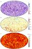 |
Fig. 13 Similar to Fig. 3, but for model A-Pr10-N3. |
| In the text | |
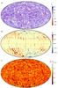 |
Fig. 14 Similar to Fig. 3, but for model NA-Pr1-N6. |
| In the text | |
|
Fig. 15 Similar to Fig. 11, but for model NA-Pr1-N6. Light curves are based on the instant shown in Fig. 14. |
| In the text | |
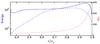 |
Fig. 16 Similar to Fig. 5, but for model NA-Pr1-N6. |
| In the text | |
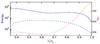 |
Fig. 17 Similar to Fig. 5, but for model S-Pr1-N5. |
| In the text | |
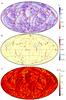 |
Fig. 18 Similar to Fig. 3, but for model S-Pr1-N5. |
| In the text | |
Current usage metrics show cumulative count of Article Views (full-text article views including HTML views, PDF and ePub downloads, according to the available data) and Abstracts Views on Vision4Press platform.
Data correspond to usage on the plateform after 2015. The current usage metrics is available 48-96 hours after online publication and is updated daily on week days.
Initial download of the metrics may take a while.