| Issue |
A&A
Volume 573, January 2015
|
|
|---|---|---|
| Article Number | A133 | |
| Number of page(s) | 13 | |
| Section | Astronomical instrumentation | |
| DOI | https://doi.org/10.1051/0004-6361/201423492 | |
| Published online | 14 January 2015 | |
Measuring the continuum polarization with ESPaDOnS⋆
1
Instituto Nacional de Pesquisas Espaciais/MCT,
Avenida dos Astronautas 1758,
São José dos Campos, SP, 12227-010, Brazil
e-mail: This email address is being protected from spambots. You need JavaScript enabled to view it.
, This email address is being protected from spambots. You need JavaScript enabled to view it.
2
Instituto Geofísico del Perú, Área Astronomía,
Calle Badajoz 169, Lima, Perú
3
Laboratório Nacional de Astrofísica (LNA/MCTI),
Rua Estados Unidos, 154,
Itajubá, MG, Brazil
Received: 23 January 2014
Accepted: 10 November 2014
Abstract
Aims. Our goal is to test the feasibility of obtaining accurate measurements of the continuum polarization from high-resolution spectra using the spectropolarimetric mode of ESPaDOnS.
Methods. We used the new pipeline OPERA to reduce recent and archived ESPaDOnS data. Several polarization standard stars and science objects were tested for the linear mode. In addition, the circular mode was tested using several objects from the archive with expected null polarization. Synthetic broad-band polarization was computed from the ESPaDOnS continuum polarization spectra and compared with published values (when available) to quantify the accuracy of the instrument.
Results. The continuum linear polarization measured by ESPaDOnS is consistent with broad-band polarimetry measurements available in the literature. The accuracy in the degree of linear polarization is around 0.2−0.3% considering the full sample. The accuracy in polarization position angle using the most polarized objects is better than 5°. Consistent with this, the instrumental polarization computed for the circular continuum polarization is also between 0.2−0.3%. Our results suggest that measurements of the continuum polarization using ESPaDOnS are viable and can be used to study many astrophysical objects.
Key words: polarization / instrumentation: polarimeters / techniques: polarimetric / stars: pre-main sequence
Based on observations obtained at the Canada-France-Hawaii Telescope (CFHT) which is operated by the National Research Council of Canada, the Institut National des Sciences de l’Univers of the Centre National de la Recherche Scientique of France, and the University of Hawaii.
© ESO, 2015
1. Introduction
ESPaDOnS is a bench-mounted high-resolution echelle spectrograph and spectropolarimeter which was designed to obtain a complete optical spectrum from ultraviolet to near-infrared wavelengths in a single exposure (Donati 2003; Manset & Donati 2003). This is installed at the 3.6 m Canada-France-Hawaii Telescope (CFHT) in Hawaii. Three operational modes are available in ESPaDOnS: object spectroscopy, sky and object spectroscopy, and spectropolarimetry. The first mode reaches a resolving power of 80 000, and the others up to 65 000.
Polarimetry with ESPaDOnS1 was initially conceived to detect linear and circular polarization along line profiles (see, e.g., Wade et al. 2005 and Harrington & Kuhn 2008). The evaluation of the feasibility of measuring the continuum polarization during the earlier ESPaDOnS commissioning was not conclusive. A high crosstalk between the Stokes parameters associated with the ESPaDOnS’ optics and losses of light over the entrance of the optical fibers were claimed by the ESPaDOnS team as factors that would play against reliable continuum polarization measurements2. In consequence, the Libre-ESpRIT pipeline (Donati et al. 1997), which has been routinely applied to ESPaDOnS data over the last years, gave priority to the line effect detection offering as default spectropolarimetry with the continuum removed.
We present new results on continuum polarization measurements using ESPaDOnS. A sample of objects, including polarimetric standard stars and science objects with previously measured polarization, was used for this purpose. The new reduction software for ESPaDOnS data, OPERA3 (Martioli et al. 2012), was used in these tests. This pipeline offers the possibility of computing the continuum polarization for ESPaDOnS data.
In Sect. 2 we investigate possible sources of instrumental polarization in the ESPaDOnS polarimetric unit and we present simulations to assess this question. Section 3 describes the data used in this work including archived and original measurements. The reduction steps processed by OPERA are explained in Sect. 4. The mathematical procedures used by OPERA to compute the Stokes parameters are shown in Sect. 5. The results of the continuum polarimetry are presented in Sect. 6 along with the computed synthetic broad-band polarimetry for the sample. A comparison between the different methods implemented by OPERA to compute the polarization is also shown. The perspectives of scientific cases that will benefit from this study are shown in Sect. 7. The conclusions are summarized in Sect. 8.
2. Instrumental limitations of ESPaDOnS when measuring continuum polarization
Donati et al. (1999) affirmed that the “MuSiCoS spectropolarimeter can in principle also estimate continuum polarization in stellar spectra... The main problem here consists in reducing true and spurious instrumental polarisation to a minimum”. ESPaDOnS has a very similar design to MuSiCoS. Therefore, if the instrumental effects degrading accuracy and precision of polarization measurements using ESPaDOnS are understood, one can efficiently reduce and/or quantify them and perform reliable measurements of continuum polarization using this instrument. In this section we discuss these effects when they originate after light has entered the polarimetric unit. We also present simulations including some of these issues.
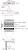 |
Fig. 1 Optical path of the polarimetric unit of ESPaDOnS. |
Figure 1 illustrates the optical path of the polarimetric unit of ESPaDOnS, where the elements that may introduce spurious polarization are shown. Figure 1 also shows the symbols representing the Mueller matrices associated with each optical element, some of which are used in our simulations.
Mueller matrix calculus can be applied to simulate the net effect of polarization
introduced by the optical train in the input light. This set of matrix transformations must
be organized in the correct order and then applied to the four-component Stokes vector
describing the input light to obtain the output intensity of each measured beam of ESPaDOnS.
Adopting the same definitions as in de la Chevrotiére et al. (2013), the simulated output beam is given by [ So ] = [
Io,Qo,Uo,Vo
], which can be calculated
as![Mathematical equation: \begin{equation} [{\bf S}_{o}] = [P][{\bf S}_{i}], \end{equation}](/articles/aa/full_html/2015/01/aa23492-14/aa23492-14-eq4.png) (1)where the input beam is given by
[ Si ]
= [
Ii,Qi,Ui,Vi
], and the transformation matrix [ P ] is given by the product
between all Mueller matrices shown in Fig. 1, i.e.,
(1)where the input beam is given by
[ Si ]
= [
Ii,Qi,Ui,Vi
], and the transformation matrix [ P ] is given by the product
between all Mueller matrices shown in Fig. 1, i.e.,
![Mathematical equation: \begin{eqnarray} [P]_{\perp} &=& [A_{\perp}][A^{c}_{\perp}][P_{\perp}]R(-\phi)][M_{\lambda/2}][ R(\phi)]\notag \\ &&\times \,[M_{\lambda/4}][R(-\theta)][M_{\lambda/2}][ R(\theta)] [H][C][P_{\rm source}], \end{eqnarray}](/articles/aa/full_html/2015/01/aa23492-14/aa23492-14-eq7.png) (2)and
(2)and
![Mathematical equation: \begin{eqnarray} [P]_{\parallel} &=& [A_{\parallel}][A^{c}_{\parallel}][P_{\parallel}]R(-\phi)] [M_{\lambda/2}][ R(\phi)] \notag\\ &&\times\, [M_{\lambda/4}][R(-\theta)] [M_{\lambda/2}][ R(\theta)] [H][C][P_{\rm source}], \end{eqnarray}](/articles/aa/full_html/2015/01/aa23492-14/aa23492-14-eq8.png) (3)where [ P ] ⊥ and
[ P ]
∥ are the perpendicular and parallel components.
(3)where [ P ] ⊥ and
[ P ]
∥ are the perpendicular and parallel components.
The first element shown in Fig. 1 is the atmospheric ersion corrector (ADC), which is an optical device that may present some stress birefringence in its optical parts, introducing spurious crosstalk polarization. The crosstalk matrix above is represented by [ C ]. Crosstalk is an instrumental artifact that may appear in both continuum and line polarization measurements. It is the conversion between fluxes in different Stokes parameters. Another possible source of crosstalk polarization is the inaccuracy of the positioning of the rotating rhombs. In ESPaDOnS, the total crosstalk between linear and circular polarization has been monitored for several years. It was reduced from 10% to 0.3% in 2009, as decribed in the ESPaDOnS homepage and Barrick et al. (2010). The present crosstalk represents a very small fraction of a given polarized source, which can be considered negligible in the study presented here. Hence, we are not concerned about crosstalk effects and for the moment we will just ignore the contribution from both [ C ] and from the positioning inaccuracy in θ and φ. The interested reader may consult Bagnulo et al. (2009; 2012), de la Chevrotiére et al. (2013), or Ilyin (2012) for a quantitative discussion and procedures to remove crosstalk from spectropolarimetric measurements.
According to the ESPaDOnS homepage4, there are two main factors that prevent reliable continuum polarization measurements:
-
1.
Instrumental polarization can occur when the stellar light enters the hole of the pierced mirror, where a non-uniform illumination of the edges of the hole introduces polarization. This effect can be accounted for by matrix [ H ]. This is expected to depend on the position of the star relative to the center of the entrance hole and on the source extension. As mentioned in the ESPaDOnS homepage this effect can be minimized by either improving guiding or using integration times where random guiding errors can be averaged out. This effect is also reduced under poor seeing conditions, where the illumination function is smoother at the edges, reducing the amplitude of asymmetries caused by decentralization of the source with respect to the hole. The polarization matrix [ H ] is somewhat difficult to model, since one needs to know the polarizing properties of the metallic surface of the pierced mirror. For this reason we decided to address this issue by inspecting the dependence between the spurious polarization and seeing conditions from our dataset. This is discussed in Sect. 6.
-
2.
The second effect occurs after the beam is split by the Wollaston prism. We note that at this stage the light beam has already passed the polarizer and analyzers and therefore the polarimetry is affected only by Stokes I. There are two problems associated with this stage. First, each of the two resultant source images reaches a different optical fiber. If each beam is not the same distance from the fiber center, then the fluxes entering each fiber will be different. This effect is accounted for by a pair of attenuation matrices,
![Mathematical equation: \hbox{$[A^{c}_{\perp}]$}](/articles/aa/full_html/2015/01/aa23492-14/aa23492-14-eq15.png) and
and
![Mathematical equation: \hbox{$[A^{c}_{\parallel}]$}](/articles/aa/full_html/2015/01/aa23492-14/aa23492-14-eq16.png) . Second, the differences in the
transmission of the two fibers will also appear as an instrumental spurious
polarization. This effect is accounted for by the attenuation matrices,
[ A⊥
] and [
A∥ ], which will introduce fiber
transmission losses.
. Second, the differences in the
transmission of the two fibers will also appear as an instrumental spurious
polarization. This effect is accounted for by the attenuation matrices,
[ A⊥
] and [
A∥ ], which will introduce fiber
transmission losses.
and , p depends on the fraction of light collected by the
fiber and should also be a function of guiding errors and seeing conditions. For the sake of
simplicity, we assume in the simulations that guiding errors are random and thus are
averaged out over an exposure. We also disregard the dependence on atmospheric seeing
conditions. According to Sect. 6.1.3, its impact is
negligible in median seeing conditions at the CFHT site (about
0 7),
given that appropriated integration times are used. We also note that the aperture entrance
for ordinary and extraordinary beams is 100 μm, which corresponds to
158,
more than twice the average seeing.
7),
given that appropriated integration times are used. We also note that the aperture entrance
for ordinary and extraordinary beams is 100 μm, which corresponds to
158,
more than twice the average seeing.
For the present simulation we are only concerned about factors [ A⊥ ] and [ A∥ ], for which the attenuation parameter p is given by the fiber transmission, T. Optical fiber transmissions can vary due to slight differences in the fiber optical path caused by different torsions or temperatures. ESPaDOnS is equipped with fiber scramblers working at 30 Hz and amplitude of 1 mm. This minimizes the transmission variations due to torsions.
All the above effects are expected to vary slowly with wavelength. Therefore, if the observer is interested in a small portion of the spectra, for example spectral lines studies, the underlying polarization continuum can be subtracted and any instrumental polarization will also be removed. This is the standard procedure adopted in ESPaDOnS data reduction.
To simplify and isolate the possible sources of errors we have only considered here the
effects caused by optical transmission losses in the fibers. In this sense, we consider that
a given fiber upon a movement will present a variation in the throughput. If the fiber
transmission is given by T then the actual transmission after a given movement
is given by T ±
δT, where δT is the square root of the variance of transmission
caused by one movement of the fiber, assuming that the fiber transmission changes randomly
with each movement. By assuming a normal distribution for the fiber transmission, the
amplitude of the variance of transmission after a given number of movements N is given
by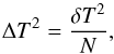 (4)where N =
fsTexp, with
fs
being the frequency of movements or the fiber scrambler frequency in Hz and Texp being the
integration time in seconds. The final variance for the fiber transmission at the end of an
exposure is then given by
(4)where N =
fsTexp, with
fs
being the frequency of movements or the fiber scrambler frequency in Hz and Texp being the
integration time in seconds. The final variance for the fiber transmission at the end of an
exposure is then given by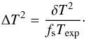 (5)Equation (5) shows that transmission uncertainty is inversely proportional to the
square root of integration time. By reducing the uncertainty in fiber transmission there
should also be an improvement in the polarimetric precision in what concerns the
instrumental polarization introduced by variations in T.
(5)Equation (5) shows that transmission uncertainty is inversely proportional to the
square root of integration time. By reducing the uncertainty in fiber transmission there
should also be an improvement in the polarimetric precision in what concerns the
instrumental polarization introduced by variations in T.
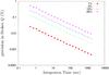 |
Fig. 2 Simulations of polarimetric precision in degree of polarization for Stokes Q versus integration time. These simulations only consider the effects caused by variability in fiber transmission. These results were obtained from 500 iterations, where we used four different values for the uncertainty in fiber transmission (δT), 1%, 5%, 10%, and 20%, as indicated in the legend. |
To quantify this effect we have run simulations where we adopted a nominal mean fiber transmission of T = 80%, which is the ESPaDOnS fiber transmission at λ = 600 nm. The simulations are run for an unpolarized source that enters the optical train. Then we apply the Mueller calculus to estimate the net effect of polarization from all components explained above to obtain the resulting flux for each beam (parallel and perpendicular) in each exposure. This procedure is repeated four times considering the typical number of exposures used by ESPaDOnS to measure each Stokes parameter.
Then the resulting fluxes are used as input to the OPERA pipeline where the polarization is calculated using the same algorithm as in real measurements. The simulations are run for 500 measurements of polarization, where we obtain the mean degree of polarization ⟨ P ⟩ and the standard deviation σP. The latter represents a quantitative measurement of the precision in polarization. We run the same simulations for four different values of transmission uncertainty in one movement of the fiber: δT = 1%, 5%, 10%, and 20%. Figure 2 shows the results of these simulations. It shows that polarimetric precision improves significantly for longer integration times, where for the highest uncertainty considered in fiber transmission of δT = 20%, integration times longer than 10 s provide a polarimetric precision better than 0.1%.
2.1. Comments about 2005 commissioning data
The ESPaDOnS webpage5 shows measurements of γ Cas (HD 5394) obtained in September 2005 as part of a commissioning run to test the stability of continuum polarization measurements with ESPaDOnS. We note that γ Cas is not an unpolarized star. It is a Be star and its polarization is around 1% and variable at a level of 0.10−0.15% (Piirola 1979). For the spectral range where λ> 540 nm these data present high levels of instrumental polarization that reach up to 10%. However for the spectral range where λ< 540 nm this variation remains below <2%. These observations have used integration times of 5 s. The levels of instrumental polarization in this experiment are well above the precision in polarization calculated in the simulations discussed in this section, and therefore cannot be explained by transmission losses in the fibers of up to 20%. However, ESPaDOnS has been through two significant upgrades since these measurements were done, which should be taken into account.
The first upgrade was the replacement of the ADC triplet lenses, which occurred in two stages. The first replacement was installed in June 2006 and the second replacement was installed in October 2008. The old ADC presented high levels of birefringence and optical imperfections due to excessive stress in the optical parts. This work is well explained in Barrick et al. (2010).
The second upgrade was the installation of new fibers and connectors, which occurred in June 2006. During the commissioning mentioned above ESPaDOnS had a spare fiber bundle installed, which replaced the original bundle between June 2005 and Feb. 2006 (see the ESPaDOnS webpage). This spare bundle exhibited a throughput loss of 0.4 mag, which represents a change of about 45% in flux.
We have two hypotheses that can explain the high levels of polarization seen in the commissioning data which agrees with both upgrades. The first is that imperfections in the ADC lenses could cause chromatic aberration in the star point spread function (PSF), which could introduce a spectral dependency in the alignment of the star with respect to the entrance hole. This could propagate to a misalignment between the two images produced by the Wollaston prism and the two fiber inputs as well. The ESPaDOnS guider uses a SCHOTT/BG38 low pass filter to select visible light6, with cut-off wavelength starting at λ> 550 nm7.
Log of observations and archived data.
Synthetic optical broad-band polarimetry using ESPaDOnS data and literature values.
The detector for guiding is a Finger Lake Instrumentation EEV CCD of type CCD47-10, which has peak efficiency at about λ = 510 nm8. Both efficiencies combined give a maximum in about the same spectral range where ESPaDOnS presents best performance in continuum polarimetric precision seen in the commissioning data. This makes us believe that centering works correctly for spectral regions where the guider is most sensitive. Chromatic effects caused by the ADC produces a degradation for other spectral ranges. This effect has probably been fixed (or minimized) after the ADC was replaced.
The second hypothesis is that the old fibers presented significantly higher throughput losses (δT> 45%), which combined with the short integration time of 5 s could have caused the high levels of spurious polarization seen in those data. In either case the problems have been mitigated and this signature does not seem to be present in recent data, obtained after the ADC and fiber repairs, as will be shown in subsequent sections.
3. Data description
In this section, we describe the data used to demonstrate the feasibility of measuring continuum polarization using ESPaDOnS. We present the linear and circular polarization data separately.
3.1. Linear polarization
The dataset for linear polarization is composed of original observations of Herbig AeBe (HeAeBe) stars gathered with ESPaDOnS at CFHT on semesters 2011A and 2011B (Proposal IDs 11AB04 and 11BB05). This program was initially proposed to measure the linear polarization across the Hα line. The results concerning the Hα measurements will be published in a separate paper. A total of nine HeAeBe stars were measured and a log of observations is shown in Table 1. All the HeAeBe stars have optical linear polarization published (Rodrigues et al. 2009) which allows us to do a proper comparison.
In order to test the capability of the OPERA software to reduce archived data of ESPaDOnS and enlarge our sample, we selected a couple of HeAeBe stars from the CFHT database9 (Proposal ID 09AH10). These stars (HD 144432 and HD 150193) also have previously published optical polarimetry (Rodrigues et al. 2009). Finally, two polarimetric standard stars from the Atlas of HST Polarimetric Calibration Objects (Turnshek et al. 1990) were measured using the same ESPaDOnS configuration in the 2011B semester as part of an independent program (Proposal ID 11BE95). One of them is the unpolarized star 73 Cet and the other one is the polarized star HD 19820. These additional four objects are included in Table 1.
Our sample spans V magnitude between 4.3 and 10.4 mag. The archived data (observed in 2009A) and the 2011A HeAeBe stars were observed using the fast readout mode of ESPaDOnS. The rest of our sample (2011B) was observed using the normal readout mode, which includes a slightly larger overhead between individual exposures. The archived data were taken using the old ESPaDOnS detector EEV1 and the rest of the sample with the new and enhanced detector Olapa. The integration time (IT) by individual frame is indicated in Table 1. Considering that a set of eight frames is needed to characterize completely a linear spectropolarimetric measurement with ESPaDOnS, this time must be multiplied by eight to obtain the total observation time (without overheads).
The signal-to-noise ratio (S/N) per CCD pixel for the order no. 35 (centered at 647 nm and near the Hα line) is also shown in Table 1. This S/N is computed by single frame using the Libre-ESpRIT pipeline and recorded in the image headers. All the objects in our sample except three have S/N higher than 150. Finally, the seeing value for each measurement is also indicated in Table 1. The quoted value is the average from the values during the observation time as it appeared in the night report for each program, when available.
As mentioned before, our sample has previously published broad-band polarization and the full polarization range goes from 0.04% (PDS 080) to 4.8% (HD 150193 and HD 19820; see Table 2). We believe that this interval is appropriate for testing the continuum linear polarization in most common polarization levels of astrophysical objects.
3.2. Circular polarization
We selected additional objects from the CFHT archive to test the circular continuum polarization. A total of seventeen measurements from eleven objects were reduced using Opera to compute V Stokes spectra. This subsample is also shown in Table 1. The sources include two objects (HD 197770 and HD 194279) used by Cox et al. (2011) to characterize spectropolarimetric features of diffuse interstellar bands, a pole-on Be star (HD 208057, Hayes 1980), a non-magnetic standard star (HD 175362, Donati et al. 1997), three linear polarized standard stars observed in V Stokes (HD 147084, HD 198478, HD 204827), and four bright sources to test the short integration times (Sirius, HD 62509, HD 98485, and Vega).
In general, all these sources are expected to show null circular continuum polarization. In this sense, this can help to investigate the accuracy for the V spectra. The integration times are spanned since very short exposures (a few seconds) to long shots (up to 900 s). In particular, short integration times were chosen to test their possible correlation with a high instrumental polarization.
4. Reductions with OPERA
The OPERA software10 was used to reduce the ESPaDOnS data. We installed and ran OPERA in a Ubuntu 12.03 Linux system. An overall description of the reduction steps for OPERA can be found in Martioli et al. (2012). The complete source software is available from the OPERA homepage11.
For extracting the flux from the two polarized beams, OPERA implements the optimal extraction algorithm by Horne (1986) and Marsh (1989) using an oversampled tilted aperture. The aperture for extraction consists of a tilted rectangle, where the tilt angle is measured from a two-dimensional instrument illumination profile obtained from a calibration Fabry-Perot alignment exposure. An oversampled tilted aperture for flux extraction is required for ESPaDOnS, since it has an image slicer, which produces a tilted pseudo-slit as the dispersing element. In addition, ESPaDOnS has a limited CCD pixel size that undersamples the spectrum. The detailed algorithms for calibration and reduction of ESPaDOnS data implemented in the OPERA pipeline are thoroughly described in another paper (Martioli et al., in prep.).
A typical calibration set for the observations presented here is composed of three bias frames, one Th-Ar lamp calibration frame, one alignment frame (Fabry Perot), and a sequence of 20 halogen lamp flat frames. For each science frame, a proper reduced calibration set must be generated considering the same observation mode (Fast, Normal, or Slow) and detector (EEV1 or Olapa).
Each Stokes parameter (Qλ, Uλ, or Vλ) is obtained by reducing four single frames in proper positions of the retarders. After this process, OPERA yields the Qλ, Uλ, or Vλ spectra and the associated errors. In the case of linear polarization, these spectra were conveniently adapted to be read by the specpol12 package, which allowed us to show multiplots including intensity (Iλ), polarization (Pλ), and position angle (PAλ) spectra. This package allows spectra binning using a variable bin size having a constant polarization error per bin. The normalized intensity spectra were directly extracted from the products yielded by the Libre-ESpRIT pipeline. Several telluric absorption bands are present in these spectra. For our purposes, the correction for telluric lines is not necessary.
5. Measuring the polarization
A detailed description of the procedure to measure the polarization using a simple polarimeter can be found in Bagnulo et al. (2009). In summary, two different methods are available to obtain any of the Stokes parameters (Q, U, or V): the ratio and difference methods. These two methods are implemented in the OPERA software. The linear polarization is a function of two Stokes parameters, Q and U, and the circular polarization is given by V. Each of these parameters is computed using four independent exposures gathered in different positions of the retarders, which rotate the polarization plane of the incident beam. The polarimetric mode of ESPaDOnS used a combination of three Fresnel rhombs as retarders. Two of them rotate (with angles φ1 and φ3) and define the net polarization plane to be measured. In each exposure two spectra are recorded with orthogonal polarization states following the splitting done by the analyzer (a Wollaston prism).
It can be shown that the transmitted intensity of light passing through the polarimetric
unit of ESPaDOnS, is given by ![Mathematical equation: \begin{eqnarray} I_\pm(\phi_1,\phi_3) &=& \frac{I_{*}}{2} [1 \pm Q \cos 4 \phi_1 \cos 4 \phi_3 \notag \\ \label{eq.itoff} &&\pm\, U \sin 4 \phi_1 \cos 4 \phi_3 \mp V \sin 4 \phi_3], \end{eqnarray}](/articles/aa/full_html/2015/01/aa23492-14/aa23492-14-eq63.png) (6)where I∗ is the incident
intensity, and φ1 and φ3 are the
directions of the retarder’s optical axes. The signals indicate the intensities of the
measured orthogonal beams produced by the analyzer splitting. All these directions are
measured with respect to the orientation of the instrument.
(6)where I∗ is the incident
intensity, and φ1 and φ3 are the
directions of the retarder’s optical axes. The signals indicate the intensities of the
measured orthogonal beams produced by the analyzer splitting. All these directions are
measured with respect to the orientation of the instrument.
In this sense, a combination of four pairs of rotations of the retarders (φ1/φ3 =
0°/0°,
90°/45°, 45°/90°, and 135°/135°) are
needed to measure Qλ and additional four
combinations (22 5/0°, 1125/45°, 675/90°, and
1575/135°) are used to measure Uλ. For V,
four combinations are needed: (0°/675,
90°/225,
45°/225,
and 135°/675).
This procedure yields a set of eight spectra for each computed Stokes parameter.
5/0°, 1125/45°, 675/90°, and
1575/135°) are used to measure Uλ. For V,
four combinations are needed: (0°/675,
90°/225,
45°/225,
and 135°/675).
This procedure yields a set of eight spectra for each computed Stokes parameter.
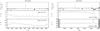 |
Fig. 3 ESPaDOnS spectropolarimetry of the HeAeBe stars HD 144432 and HD 150193 gathered from the CFHT archive. The spectra show the normalized total flux (top), polarization level (middle), and polarization position angle (bottom, θ = PA) binned using a variable bin size with a constant polarization error per bin of 0.1%. |
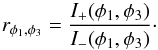
Following the ratio method, we define the ratio between the orthogonal polarization
intensities in a given combination of the retarders position as follows:
 Then, the Stokes parameters can be obtained
from
Then, the Stokes parameters can be obtained
from ![Mathematical equation: \begin{eqnarray*} Q &=& \frac{ R_{Q} - 1}{ R_{Q} + 1}, \;\; \textrm{being} \;\; R^{4}_{Q} = \left(\frac{r_{0,0}}{r_{90,45}}\right) \left(\frac{r_{135,135}}{r_{45,90}}\right),\;\;\;\;\;\;\;\;\;\;\;\; \\[-1mm] U &=& \frac{ R_{U} - 1}{ R_{U} + 1}, \;\; \text{being} \;\; R^{4}_{U} = \left(\frac{r_{22.5,0}}{r_{112.5,45}}\right) \left(\frac{r_{157.5,135}}{r_{67.5,90}}\right), \rm{and} \\[-1mm] V &=& \frac{ R_{V} - 1}{ R_{V} + 1}, \;\; \text{being} \;\; R^{4}_{V} = \left(\frac{r_{0,67.5}}{r_{90,22.5}}\right) \left(\frac{r_{135,67.5}}{r_{45,22.5}}\right)\cdot \end{eqnarray*}](/articles/aa/full_html/2015/01/aa23492-14/aa23492-14-eq70.png) The degree (P) and the
position angle (PA) of the linear polarization are determined from the following
expressions:
The degree (P) and the
position angle (PA) of the linear polarization are determined from the following
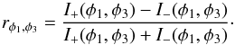
expressions: 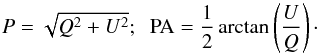 (7)In the same way, the difference method can be
applied if we define the ratio between the difference and the sum of the two orthogonal
polarization intensities in a given combination of the retarders position, as follows:
(7)In the same way, the difference method can be
applied if we define the ratio between the difference and the sum of the two orthogonal
polarization intensities in a given combination of the retarders position, as follows:
 Then, the Stokes parameters can be obtained
from
Then, the Stokes parameters can be obtained
from ![Mathematical equation: \begin{eqnarray*} Q = \frac{1}{4} \left[\left(r_{0,0} - r_{90,45}\right) - \left(r_{45,90} - r_{135,135}\right)\right],\;\;\;\;\;\;\;\;\;\;\;\;\;\;\;\;\; \end{eqnarray*}](/articles/aa/full_html/2015/01/aa23492-14/aa23492-14-eq73.png)
![Mathematical equation: \begin{eqnarray*} U = \frac{1}{4}\left[\left(r_{22.5,0} - r_{112.5,45}\right) - \left(r_{67.5,90} - r_{157.5,135}\right)\right],\;\; \rm{and} \end{eqnarray*}](/articles/aa/full_html/2015/01/aa23492-14/aa23492-14-eq74.png)
![Mathematical equation: \begin{eqnarray*} V = \frac{1}{4}\left[\left(r_{0,67.5} - r_{90,22.5}\right) - \left(r_{45,22.5} - r_{135,67.5}\right)\right].\;\;\;\;\;\;\;\;\;\;\;\; \end{eqnarray*}](/articles/aa/full_html/2015/01/aa23492-14/aa23492-14-eq75.png) In this work, the ratio method was used to
compute the continuum (linear and circular) polarization using OPERA. A comparison between
the two methods is presented in Sect. 6.1.1.
In this work, the ratio method was used to
compute the continuum (linear and circular) polarization using OPERA. A comparison between
the two methods is presented in Sect. 6.1.1.
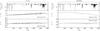 |
Fig. 6 As Fig. 3 for the standard stars 73 Cet (unpolarized) and HD 19820 (polarized) gathered with ESPaDOnS in the 11BE95 proposal. |
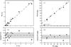 |
Fig. 7 Comparison of synthetic V broad-band linear polarization from
ESPaDOnS and literature values. a) The abscissa is the degree of
polarization (P) measured using ESPaDOnS. The ordinate is the
literature value (Plit). The dashed line represents
Plit = P. b) The
residual (Plit
− P). The gray zone indicates a one-sigma
dispersion around the mean value: 0 ± 0.23% (dashed line). c) The abscissa is the polarization
position angle (PA) measured using ESPaDOnS. The ordinate is the literature value
(PAlit). The
dashed line represents PAlit = PA. The black dots are objects with
P>
0.5% and crosses with P< 0.5%. The PA variable HD 144668 is labeled. d) The residual
(PAlit − PA)
only for objects with P> 0.5%. The gray zone indicates a one-sigma
dispersion around the mean value: −3 |
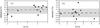 |
Fig. 8 Residuals in Stokes parameters between synthetic V broad-band linear polarization from ESPaDOnS and literature values. a) The abscissa is the Q Stokes parameter measured using ESPaDOnS. The ordinate is the residual (Qlit − Q). The gray zone indicates a one-sigma dispersion around the mean value: 0.07 ± 0.18% (dashed line). b) The abscissa is the U Stokes parameter measured using ESPaDOnS. The ordinate is the residual (Ulit − U). The gray zone indicates a one-sigma dispersion around the mean value: − 0.08 ± 0.21% (dashed line). |
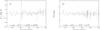 |
Fig. 9 Residuals between the ratio and difference methods computed by OPERA for the high polarized object HD 150193. a) Degree of polarization; b) position angle. The spectra are binned using a variable bin size with a constant polarization error per bin of 0.1%. The mean values and one-sigma dispersion are indicated in each case. |
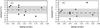 |
Fig. 10 Residuals in Stokes parameters versus seeing values for Q a) and U b). The dashed line and gray zones are as in Fig. 8. |
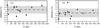 |
Fig. 11 Residuals in Stokes parameters versus integration times for Q a) and U b). The dashed line and gray zones are as in Fig. 8. |
6. Results
6.1. Linear polarization
Figures 3−6 show the results for the spectropolarimetry of our linear polarization sample (Table 1). The spectra are binned to enhance the signal-to-noise ratio. We selected a polarimetric error of 0.1% per bin as a good compromise to show the data properly.
Our sample includes HeAeBe stars with very low polarization levels such as HD 144432, PDS 395, and PDS 080. Interestingly, the mean level of the binned polarization spectrum of PDS 395 (Fig. 4) is lower than 0.1%, which is a good example of the ability of ESPaDOnS to detect low polarizations. On the other hand, high polarization levels (up to ~5%) are well sampled, as are the cases of the HeAeBe star HD 150193 (Fig. 3) and the polarized standard star HD 19820 (Fig. 6).
HeAeBe stars are known to exhibit time-variability in flux and polarization. Hence caution must be taken when comparing measurements, because possible differences may be intrinsic to the object and not due to observational uncertainties. We looked for previous broad-band polarization measurements of our HAeBe sample to check for variability and only in one case confirmed variability was found (see below).
In order to facilitate the comparison with the literature and test the quality of the continuum linear polarization from ESPaDOnS, we calculate synthetic VRI broad-band polarization averaging the Stokes parameters (Qλ and Uλ) between the cut-on and cut-off wavelengths associated with these standard broad-band filters. The intervals were 5070−5950Å, 5890−7270Å, and 7315−8805Å for the V, R, and I filters, respectively. The synthetic values are shown in Table 2 along with the literature values when available.
All the HeAeBe stars in our sample have optical polarization (at V filter) previously measured by Rodrigues et al. (2009). The two polarimetric standard stars (73 Cet and HD 19820) have published values by Schmidt et al. (1992).
In Fig. 7, we compare the polarization level at V band of the objects in our sample with their published values (Plit) as given in Table 2. The polarization degree comparison (Fig. 7a) shows a good agreement between ESPaDOnS data and the results published in the literature. The polarimetric accuracy is preserved for lower and higher values of polarization. The slope one is included to help the comparison. Considering all objects in the sample, the residual of the polarization measurements (Fig. 7b) has a mean zero with a one-sigma dispersion of 0.23%. In a few cases (3 out of 13), residuals of 0.4% are found. This result gives us confidence that accuracies as low as 0.2−0.3% can be obtained measuring the continuum linear polarization with ESPaDOnS.
As discussed in Sect. 2, small ITs must prevent a reliable measurement of the continuum polarization. The polarization degree measured by ESPaDOnS for the unpolarized standard star 73 Cet is around 0.5% along the full spectrum (Fig. 6, left). This level is well above the published polarization (0.1%, Schmidt et al. 1992) considering our quoted errors. The S/N for this object (see Table 1) is similar to other well sampled objects in our sample and this does not seem to be the origin of the discrepancy. However, an inspection of the integration times reveals that this object is the only one in our sample with a small IT (15 s). Similar ITs were used by the ESPaDOnS team during the earlier commissioning13. We believe that such short ITs are not sufficient to average out the modal noise present in the optical fibers. This is confirmed by the results for circular continuum polarization presented in the next section.
We also computed the residuals between the ESPaDOnS polarization position angle and the published values (Fig. 7c). Caution must be taken with this comparison because low polarization levels cause high indetermination in the PA. For this reason, we computed the residuals in PA only for objects with a high degree of polarization (larger than 0.5%, Fig. 7d). Using this criterion, five objects were removed from the subsequent analysis.
In particular, the PA residual of HD 144668 (~30°) also fitted our criteria of higher P. Nevertheless, this object is the only source in our sample that seems to show historical intrinsic variability in PA14 (Hutchinson et al. 1994, Bhatt 1996) and it was not included in Fig. 7d.
The residuals in PA have a mean of −33
±
43.
Therefore, the accuracy in PA for measurements of the continuum linear polarization using
ESPaDOnS is better than 5°. In
particular, the constancy of the PA along the spectra for the polarized standard star
(HD 19820, Fig. 6, right) and its comparison with the published broad-band values (see Table
2) indicate a very reliable result.
In order to confirm this issue, we computed the residuals between the V broad-band polarization measured by ESPaDOnS and the literature values using the Stokes parameters (Q = P × cos(2PA), U = P × sin(2PA)). Figure 8a shows the residual in Q with a mean of 0.07 ± 0.18%. The residual in U (Fig. 8b) has a similar dispersion with a mean of − 0.08 ± 0.21%. In this analysis, the star HD 144668 has also been excluded for the reasons explained above. These results confirm our previous results, where accuracies associated with the polarization are 0.2−0.3%. The mean values of Q and U are consistent with zero, showing no bias to positive or negative values, within the dispersion. These mean values can be interpreted as maximum limits for the instrumental polarization in Q and U parameters.
In general, the comparison of the optical synthetic broad-band polarimetry indicates that accurate continuum linear polarization measurements are feasible using ESPaDOnS. The measured polarizations are consistent with the literature values.
6.1.1. Comparing ratio and difference methods
A comparison between the two methods implemented by OPERA (see Sect. 5) to compute the polarization was done for the highly
polarized object HD 150193. Figure 9 shows the residuals between the ratio and difference
methods computed in polarization degree and position angle. The residual in polarization
degree is 0.02% ± 0.05% and
in polarization angle is  . These values imply that both
methods yield similar results, whose differences are below 0.05% in polarization and
. These values imply that both
methods yield similar results, whose differences are below 0.05% in polarization and
 in PA. Hence, the results using OPERA
are independent of the method used to compute the polarization. This is consistent with
the analytical approach from Bagnulo et al. (2009).
in PA. Hence, the results using OPERA
are independent of the method used to compute the polarization. This is consistent with
the analytical approach from Bagnulo et al. (2009).
6.1.2. Polarization gradients
HeAeBe stars with unknown continuum polarization are not appropriate to study polarization gradients because they can have intrinsic polarization which is usually variable with wavelength. Hence we based our discussion on this topic using HeAeBe stars with small values of polarization, consistent with null polarization.
Figures 3−6 reveal non-negligible gradients in the polarization levels. This is especially important for low polarization levels. Considering the accuracies computed using the V broad-band and extrapolating them to lower and higher wavelengths, a conservative polarization level of 0.6% can be used as a threshold for a real detection of a particular wavelength dependence in polarization. This level must be taken with caution considering the signal-to-noise ratios used in our sample. Consistent with this, a dependence of the polarization position angle with wavelength is evident for objects with low polarizations at the level of the ESPaDOnS accuracy (~0.3%). Therefore, the gradients observed in the position angle for HD 144432, PDS 395, and PDS 080 are examples of artifacts.
Interestingly, the wavelength (λmax) for maximum polarization (Pmax) for the polarized standard star in our sample (HD 19820) computed from the ESPaDOnS spectra (λmax = 5298 Å, Pmax = 4.63%) is in excellent agreement with the published values by Schmidt et al. (1992, λmax = 5235 Å, Pmax = 4.76%). In this case, the consistency in Pmax is better than 0.15%. Moreover, the PA of HD 19820 is remarkably constant along the whole spectrum, as expected for a polarized standard star. This indicates that a PA gradient, if present, should be small. This shows that reliable wavelength dependence in polarization can be obtained for polarized objects measured by ESPaDOnS.
6.1.3. Seeing and integration time dependence
As discussed in Sect. 2, the seeing can affect the
quality of a polarization measurement. In order to verify any trend of this kind, we
check the dependence of the residuals of our measurements in each Stokes parameters with
the seeing value quoted in Table 1. This is shown
in Fig. 10. The interval of seeing sampled in our
measurements, between 05
and 08,
is very typical of CFHT conditions. No correlation is apparent in Q or
U Stokes parameters. This result suggests that the accuracy for the
linear continuum polarization does not vary considerably with the seeing, at least for
the interval covered by our sample.
Finally, the correlation between integration times and instrumental polarization in Q and U spectra was tested with the ITs quoted in Table 1. Figure 11 shows a plot of the residuals in Q and U versus IT. The minimum IT used in our sample was 15 s for the unpolarized standard star 73 Cet. This object was discussed above considering its higher residual in the polarization level. Interestingly, this is one of the two objects with both residuals (in Q and U) being above one-sigma outside the mean values. The second object is the polarized HeAeBe star PDS 545 which was observed with ~460 s. Considering that small variations in polarization are common in HeAeBe stars, the measurement of 73 Cet seems to indicate a real higher instrumental polarization associated with low integration times. Nevertheless, additional data are needed to confirm this question (see next section).
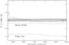 |
Fig. 12 Circular continuum polarization spectra of selected objects from the CFHT archive. Seventeen measurements are shown. The highest levels of V in two short exposures are indicated with the integration times in parenthesis. |
6.2. Circular polarization
Figure 12 shows the circular polarization spectra for the seventeen measurements from Table 1. As mentioned before, our sample includes measurements using short and long exposures. Interestingly, the short exposures show the highest levels for the V Stokes spectra. One of the bright sources (Vega) has three different measurements with IT of 1, 2, and 4 s, respectively. Figure 12 clearly shows that the 1 s measurement has the highest V level. The same effect is also observed in another bright source (Sirius) with three measurements with different ITs. The short exposure (0.6 s) also shows an extreme V value. These particular spectra are indicated in Fig. 12.
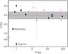 |
Fig. 13 Synthetic circular polarization for selected objects from the CFHT archive. As in Fig. 12, the highest levels are shown. The gray zone indicates a one-sigma dispersion around the mean value: − 0.01 ± 0.21%, for objects with IT ≥ 20 s. This limit is indicated by a vertical dashed line. The objects measured using the old ADC (in 2006−2008 interval) are shown with magenta dots. The more recent measurements are shown with black dots. |
Synthetic polarimetry for V Stokes parameter using ESPaDOnS data.
In order to quantify the instrumental polarization in circular polarization for the ESPaDOnS data, we computed synthetic polarization averaging the V Stokes parameter considering the full wavelength interval available in ESPaDOnS (between 4500−10 000 Å). The results are shown in Table 3. Figure 13 shows the circular polarization level versus the integration time. All the measurements with integration times higher than 20 s are below 0.3% (in absolute value). A higher dispersion happens for short IT. For IT ≥ 20 s, the average is practically zero (− 0.01%) with a dispersion of 0.2%. This is indicated by the dotted line and gray zone in Fig. 13. We confirmed that ESPaDOnS has an instrumental polarization for circular continuum polarization between 0.2−0.3%. This level is similar to our results in linear continuum polarization. Finally, evidence of a higher instrumental polarization for short integration times is also found.
As discussed in Sect. 2, a possible source of instrumental polarization was the old ADCs. To test this hypothesis, the data obtained using the ADC installed in ESPaDOnS from 2006 June to 2008 Oct. are highlighted in Fig. 13. These data actually show a higher dispersion than data obtained with the present ADC, indicating that ADC can be indeed the cause of spurious polarization in old ESPaDOnS data.
7. Perspectives
Assuming that the continuum polarimetry is feasible using ESPaDOnS, the range of scientific applications of this instrument will be widened. Continuum polarization arises in asymmetric scattering, dichroic extinction, and some non-thermal emission processes, for instance. Size distribution and chemical composition of interstellar grains can be estimated by modeling the continuum polarization wavelength dependence (see, e.g., Rodrigues et al. 1997 and Siebenmorgen et al. 2014). Continuum polarimetry can also be used to determine the geometric distribution, sizes, and nature of scatterers in circumstellar environments. Some examples are young stellar objects (Pereyra et al. 2009), Be stars (Draper et al. 2014), and binary stars (Rodrigues & Magalhães 1995). The geometry of supernovae explosions is another example of objects that can be studied using the continuum polarization measurements (Pereyra et al. 2006). The presence of spots in a stellar surface emission can break the symmetry producing a net continuum polarization (Patel et al. 2013). A classical example of extragalactic application of continuum spectropolarimetry is the discovery that the polarized flux of Seyfert 2 galaxies can reveal a Seyfert 1 spectrum (Antonucci & Miller 1985), leading to the unified model of active galactic nuclei. Synchrotron emission from active galactic nuclei can also produce optical continuum polarization (Barres de Almeida et al. 2014). In stellar astrophysics, cyclotron emission in magnetic cataclysmic variables is also a source of continuum polarization (Silva et al. 2013).
8. Conclusions
We demonstrated the ESPaDOnS’ ability to measure continuum polarization. A sample composed of HeAeBe stars with known optical polarization and polarimetric standards were used to study the linear polarization. Other objects of different kinds and with expected null circular polarization provide a sample to circular polarization analysis. We obtained the wavelength dependence of the continuum Stokes parameters for all objects. Data reduction was done using the new OPERA pipeline for ESPaDOnS data. Well sampled continuum linear polarization spectra were measured with polarization levels ranging between 0% and 5% and circular polarization around 0%.
Synthetic broad-band linear polarization computed from the ESPaDOnS spectra was compared with published values to quantify the accuracy of the instrument. The continuum linear polarization measured by ESPaDOnS is fully consistent with the broad-band polarimetry measurements already published. Our tests yielded a polarization degree accuracy around 0.2−0.3%. In turn, the accuracy in polarization position angle was better than 5°. When continuum circular polarization spectra are analyzed, instrumental polarization of 0.2−0.3% is also found for the Stokes V parameter. Our results suggest that high quality measurements of the continuum polarization are feasible with ESPaDOnS.
Many science cases would benefit from continuum polarization measurements. This justifies our study that proves the ability of ESPaDOnS to reliably measure continuum polarization.
Some of the deficiencies presented in Sect. 2 that limit accurate measurements of continuum polarization with ESPaDOnS are minimized in slit-fed low resolution spectropolarimeters (e.g., FORS). For instance, a slit-fed spectrograph does not suffer from random fiber transmission losses due to fiber torsion and misalignment between the star PSF and the fiber entrance. However, as presented in Sect. 2, we showed that fiber-fed spectrographs can be optimized for continuum polarization measurements by adopting sufficiently long integration times coupled with the frequency of the fiber scrambler, and also by implementing careful guiding to keep the alignment between the target and fiber.
Open-source Pipeline for Espadons Reduction and Analysis (OPERA), is an Open Source software reduction pipeline for the ESPaDOnS spectro-polarimeter at the Canada France Hawaii Telescope.
Version 2013/Oct/21.
specpol was originally written by A. Carciofi and is available in PCCDPACK (Pereyra et al. 2000).
See legends of Table 2.
Acknowledgments
The authors wish to thank the referee S. Bagnulo for his careful reading. His several comments and suggestions greatly helped to improve the paper. A.P. thanks FAPESP (grant 13/11473-7) and CNPq (DTI grant 382.585/07-03 associated with the PCI/MCT/ON program). A.P. is grateful to Douglas Teeple for his support to the OPERA installation. C.V.R. thanks Fapesp (grant 10/01584-8) and CNPq (grant 306103/2012-5). This research used the facilities of the Canadian Astronomy Data Centre operated by the National Research Council of Canada with the support of the Canadian Space Agency.
References
- Antonucci, R. R. J., & Miller, J. S. 1985, ApJ, 297, 621 [NASA ADS] [CrossRef] [Google Scholar]
- Bagnulo, S., Landolfi, M., Landstreet, J. D., et al. 2009, PASP, 121, 993 [NASA ADS] [CrossRef] [Google Scholar]
- Bagnulo, S., Landstreet, J. D., Fossati, L., & Kochukhov, O. 2012, A&A, 538, A129 [NASA ADS] [CrossRef] [EDP Sciences] [Google Scholar]
- Barres de Almeida, U., Tavecchio, F., & Mankuzhiyil, N. 2014, MNRAS, 441, 2885 [NASA ADS] [CrossRef] [Google Scholar]
- Barrick, G., Benedict, T., & Sabin, D. 2010, Proc. SPIE, 7735, 77354C-1 [CrossRef] [Google Scholar]
- Bhatt, H. C. 1996, A&AS, 120, 451 [NASA ADS] [CrossRef] [EDP Sciences] [Google Scholar]
- de la Chevrotiére, A., St-Louis, N., Moat, A. F. J., & the MiMeS Collaboration 2013, ApJ, 764, 171 [NASA ADS] [CrossRef] [Google Scholar]
- Donati, J.-F. 2003, in Solar Polarization 3, eds. J. Trujillo-Bueno, & J. Sanchez Almeida (San Francisco: ASP), ASP Conf. Ser., 307, 41 [Google Scholar]
- Donati, J.-F., Semel, M., Carter, B. D., Rees, D. E., & CollierCameron, A. 1997, MNRAS, 291, 658 [NASA ADS] [CrossRef] [MathSciNet] [Google Scholar]
- Donati, J.-F., Catala, C., Wade, G. A., et al. 1999, A&AS, 134, 149 [NASA ADS] [CrossRef] [EDP Sciences] [Google Scholar]
- Draper, Z. H., Wisniewski, J. P., Bjorkman, K. S., et al. 2014, ApJ, 786, 120 [NASA ADS] [CrossRef] [Google Scholar]
- Harrington, D. M., & Kuhn, J. 2008, PASP, 120, 89 [NASA ADS] [CrossRef] [Google Scholar]
- Hayes, D. P. 1980, PASP, 92, 661 [NASA ADS] [CrossRef] [Google Scholar]
- Horne, K. 1986, PASP, 98, 609 [NASA ADS] [CrossRef] [EDP Sciences] [Google Scholar]
- Hutchinson, M. G., Albinson, J. S., Barrett, P., et al. 1994, A&A, 285, 883 [NASA ADS] [Google Scholar]
- Ilyin, I. 2012, Astron. Nachr., 333, 213 [NASA ADS] [CrossRef] [Google Scholar]
- Manset, N., & Donati, J.-F. 2003, in Polarimetry in Astronomy, ed. S. Fineschi, Proc. SPIE, 4843, 425 [Google Scholar]
- Marsh, T. R. 1989, PASP, 101, 1032 [NASA ADS] [CrossRef] [Google Scholar]
- Martioli, E., Teeple, D., Manset, N., et al. 2012, in Software and Cyberinfrastructure for Astronomy II, Proc. SPIE, 8451, 84512B [CrossRef] [Google Scholar]
- Patel, M. K., Pandey, J. C., Savanov, I. S., Prasad, V., & Srivastava, D. C. 2013, MNRAS, 430, 2154 [NASA ADS] [CrossRef] [Google Scholar]
- Pereyra, A. 2000, Ph.D. Thesis, Instituto Astronômico e Geofísico, Universidade de São Paulo, Brazil [Google Scholar]
- Pereyra, A., Girart, J. M., Magalháes, A. M., Rodrigues, C. V., & de Araújo, F. X. 2009, A&A, 501, 595 [NASA ADS] [CrossRef] [EDP Sciences] [Google Scholar]
- Piirola, V. 1979, A&AS, 38, 193 [NASA ADS] [Google Scholar]
- Rodrigues, C. V., & Magalhães, A. M. 1995, in Wolf-Rayet Stars: Binaries, Colliding Winds, Evolution, eds. K. A. van der Hucht, & P. M. Williams, IAU Symp., 163, 260 [Google Scholar]
- Rodrigues, C. V., Magalhães, A. M., Coyne, G. V., & Piirola, S. J. V. 1997, ApJ, 485, 618 [NASA ADS] [CrossRef] [Google Scholar]
- Rodrigues, C. V., Sartori, M. J., Gregorio-Hetem, J., & Magalhães, A. M. 2009, ApJ, 698, 2031 [NASA ADS] [CrossRef] [Google Scholar]
- Schmidt, G. D., Elston, R., & Lupie, O. L. 1992, AJ, 104, 1563 [NASA ADS] [CrossRef] [Google Scholar]
- Siebenmorgen, R., Voshchinnikov, N. V., & Bagnulo, S. 2014, A&A, 561, A82 [NASA ADS] [CrossRef] [EDP Sciences] [Google Scholar]
- Silva, K. M. G., Rodrigues, C. V., Costa, J. E. R., et al. 2013, MNRAS, 432, 1587 [NASA ADS] [CrossRef] [Google Scholar]
- Sterzik, M. F., Bagnulo, S., & Palle, E. 2012, Nature, 483, 64 [NASA ADS] [CrossRef] [Google Scholar]
- Turnshek, D. A., Bohlin, R. C., Williamson, R. L., et al. 1990, AJ, 99, 4 [Google Scholar]
- Wade, G. A., Drouin, D., Bagnulo, S., et al. 2005, A&A, 442, L31 [NASA ADS] [CrossRef] [EDP Sciences] [Google Scholar]
All Tables
Synthetic optical broad-band polarimetry using ESPaDOnS data and literature values.
All Figures
|
Fig. 1 Optical path of the polarimetric unit of ESPaDOnS. |
| In the text | |
|
Fig. 2 Simulations of polarimetric precision in degree of polarization for Stokes Q versus integration time. These simulations only consider the effects caused by variability in fiber transmission. These results were obtained from 500 iterations, where we used four different values for the uncertainty in fiber transmission (δT), 1%, 5%, 10%, and 20%, as indicated in the legend. |
| In the text | |
|
Fig. 3 ESPaDOnS spectropolarimetry of the HeAeBe stars HD 144432 and HD 150193 gathered from the CFHT archive. The spectra show the normalized total flux (top), polarization level (middle), and polarization position angle (bottom, θ = PA) binned using a variable bin size with a constant polarization error per bin of 0.1%. |
| In the text | |
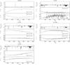 |
Fig. 4 As Fig. 3 for the HeAeBe stars gathered with ESPaDOnS in the 11AB04 proposal. |
| In the text | |
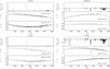 |
Fig. 5 As Fig. 3 for the HeAeBe stars gathered with ESPaDOnS in the 11BB05 proposal. |
| In the text | |
|
Fig. 6 As Fig. 3 for the standard stars 73 Cet (unpolarized) and HD 19820 (polarized) gathered with ESPaDOnS in the 11BE95 proposal. |
| In the text | |
|
Fig. 7 Comparison of synthetic V broad-band linear polarization from
ESPaDOnS and literature values. a) The abscissa is the degree of
polarization (P) measured using ESPaDOnS. The ordinate is the
literature value (Plit). The dashed line represents
Plit = P. b) The
residual (Plit
− P). The gray zone indicates a one-sigma
dispersion around the mean value: 0 ± 0.23% (dashed line). c) The abscissa is the polarization
position angle (PA) measured using ESPaDOnS. The ordinate is the literature value
(PAlit). The
dashed line represents PAlit = PA. The black dots are objects with
P>
0.5% and crosses with P< 0.5%. The PA variable HD 144668 is labeled. d) The residual
(PAlit − PA)
only for objects with P> 0.5%. The gray zone indicates a one-sigma
dispersion around the mean value: −3 |
| In the text | |
|
Fig. 8 Residuals in Stokes parameters between synthetic V broad-band linear polarization from ESPaDOnS and literature values. a) The abscissa is the Q Stokes parameter measured using ESPaDOnS. The ordinate is the residual (Qlit − Q). The gray zone indicates a one-sigma dispersion around the mean value: 0.07 ± 0.18% (dashed line). b) The abscissa is the U Stokes parameter measured using ESPaDOnS. The ordinate is the residual (Ulit − U). The gray zone indicates a one-sigma dispersion around the mean value: − 0.08 ± 0.21% (dashed line). |
| In the text | |
|
Fig. 9 Residuals between the ratio and difference methods computed by OPERA for the high polarized object HD 150193. a) Degree of polarization; b) position angle. The spectra are binned using a variable bin size with a constant polarization error per bin of 0.1%. The mean values and one-sigma dispersion are indicated in each case. |
| In the text | |
|
Fig. 10 Residuals in Stokes parameters versus seeing values for Q a) and U b). The dashed line and gray zones are as in Fig. 8. |
| In the text | |
|
Fig. 11 Residuals in Stokes parameters versus integration times for Q a) and U b). The dashed line and gray zones are as in Fig. 8. |
| In the text | |
|
Fig. 12 Circular continuum polarization spectra of selected objects from the CFHT archive. Seventeen measurements are shown. The highest levels of V in two short exposures are indicated with the integration times in parenthesis. |
| In the text | |
|
Fig. 13 Synthetic circular polarization for selected objects from the CFHT archive. As in Fig. 12, the highest levels are shown. The gray zone indicates a one-sigma dispersion around the mean value: − 0.01 ± 0.21%, for objects with IT ≥ 20 s. This limit is indicated by a vertical dashed line. The objects measured using the old ADC (in 2006−2008 interval) are shown with magenta dots. The more recent measurements are shown with black dots. |
| In the text | |
Current usage metrics show cumulative count of Article Views (full-text article views including HTML views, PDF and ePub downloads, according to the available data) and Abstracts Views on Vision4Press platform.
Data correspond to usage on the plateform after 2015. The current usage metrics is available 48-96 hours after online publication and is updated daily on week days.
Initial download of the metrics may take a while.