| Issue |
A&A
Volume 572, December 2014
|
|
|---|---|---|
| Article Number | L1 | |
| Number of page(s) | 4 | |
| Section | Letters | |
| DOI | https://doi.org/10.1051/0004-6361/201424901 | |
| Published online | 18 November 2014 | |
Resolving the stellar components of the massive multiple system Herschel 36 with AMBER/VLTI
1 Instituto de Astrofísica de Andalucía (CSIC), Glorieta de la Astronomía S/N, 18008 Granada, Spain
e-mail: This email address is being protected from spambots. You need JavaScript enabled to view it.
2 European Southern Observatory, Karl-Schwarzschild-Stra β e 2, 85748 Garching, Germany .
3 Departamento de Física, Universidad de la Serena, Av. Cisternas 1200 Norte, 204000 La Serena, Chile
4 Max-Planck-Institut für Astronomie, Königstuhl 17, 69117 Heidelberg, Germany
5 Departamento de Astrofísica, Centro de Astrobiología (INTA-CSIC), campus ESA, apartado postal 78, 28 691 Villanueva de la Cañada, Madrid, Spain
Received: 1 September 2014
Accepted: 7 October 2014
Abstract
Context. Massive stars are extremely important for the evolution of the galaxies; there are large gaps in our understanding of their properties and formation, however, mainly because they evolve rapidly, are rare, and distant. Recent findings suggest that most O-stars belong to multiple systems. It may well be that almost all massive stars are born as triples or higher multiples, but their large distances require very high angular resolution to directly detect the companions at milliarcsecond scales.
Aims. Herschel 36 is a young massive system located at 1.3 kpc. It has a combined smallest predicted mass of 45 M⊙. Multi-epoch spectroscopic data suggest the existence of at least three gravitationally bound components. Two of them, system Ab, are tightly bound in a spectroscopic binary, and the third one, component Aa, orbits in a wider orbit. Our aim was to image and obtain astrometric and photometric measurements of components Aa and Ab using, for the first time, long-baseline optical interferometry to further constrain its nature.
Methods. We observed Herschel 36 with the near-infrared instrument AMBER attached to the ESO VLT Interferometer, which provides an angular resolution of ~2 mas. We used the code BSMEM to perform the interferometric image reconstruction. We fitted the interferometric observables using proprietary IDL routines and the code LitPro.
Results. We imaged the Aa + Ab components of Herschel 36 in H and K filters. Component Ab is located at a projected distance of 1.81 mas, at a position angle of ~222° east of north, the flux ratio between components Aa and Ab is close to one. These findings agree with previous predictions about the properties of Herschel 36. The small measured angular separation indicates that system Ab and Ab may be approaching the periastron of their orbits. These results, only achievable with long-baseline near-infrared interferometry, constitute the first step toward a thorough understanding of this massive triple system.
Key words: instrumentation: high angular resolution / instrumentation: interferometers / binaries: close / stars: massive
© ESO, 2014
1. Introduction
The evolution of galaxies cannot be fully understood without studying the formation and evolution of massive stars. They are important actors in the enrichment and mixing of the interstellar medium. Therefore, they can initiate, accelerate, or impede the star and planet formation. However, despite their importance, our knowledge about their birth and evolution is still not conclusive. This is, mainly, because they spend a significant part of their main-sequence lifetime (20%) still embedded in high-extinction dust clouds, they evolve rapidly (~Ma), are rare, and typically located at large distances (≥1 kpc) (Zinnecker & Yorke 2007).
Recent studies on the multiplicity of massive stars suggest that at least 70% of them belong to binaries or high-degree multiple systems (Mason et al. 2009; Maíz Apellániz 2010; Sana & Evans 2011; Sota et al. 2014). Moreover, Sana et al. (2012) suggested that the interaction between components in massive binaries dominates the evolution of massive stars. Therefore, ignoring the role of multiplicity on the formation and evolution of massive stars introduces strong bias in star formation theories. Despite the existing body of research, our knowledge of the multiplicity of massive stars is still incomplete, in particular (a) at the upper-end of the initial mass function (IMF) and (b) at the early evolutionary stages of high-mass stars (e.g., zero-age main-sequence – ZAMS – objects). This is because observations of these systems are difficult because of their rareness and distance (e.g., HD 150136; Sanchez-Bermudez et al. 2013). Hence, studying each individual system is necessary to obtain reliable statistics of their properties. High-angular resolution techniques are therefore required to characterize them fully.
Herschel 36 is a young massive system located at 1.3 kpc (Arias et al. 2006) in the Hourglass high-mass star-forming region in the central part of the M 8 nebula. This object is responsible for most of the gas ionization in the region. Arias et al. (2010) concluded that Herschel 36 is composed of at least three main components: two of them are the stars1Ab1 (O9 V) and Ab2 (B0.5 V), which form a close binary (system Ab) with a period of 1.54 days; the third one is component Aa (O7.5 V), which is the most luminous star of the system and dominates its ionizing flux. These authors also reported strong variations in the line profile, shape, and radial velocity of the known components of Herschel 36, which indicate that component Aa and system Ab are gravitationally tied up in a wider orbit with a period of approximately 500 days and a projected semi-major axis of 3.5 mas between components Aa and Ab. The smallest spectroscopic predicted mass of the system Aa + Ab is of 19.2 + 26.0 = 45.2 M⊙. The combined luminosity of the three components of Herschel 36 agrees with the expected theoretical luminosity of three ZAMS stars (Arias et al. 2010). This evolutionary stage is very difficult to observe since it only lasts shorter than 1 Ma in stars of such high mass. Moreover, in addition to the Aa + Ab components, there is a fourth star located at 0.25′′ (Herschel 36 SE; Goto et al. 2006) and other stars several arcseconds away that may also be gravitationally bound to Herschel 36. Because its location, multiplicity, and role in the nebula, this system has therefore been compared to θ1 Ori C (Kraus et al. 2009) in the Orion Trapezium. The complete characterization of Herschel 36 may provide new links between the observed properties and the evolutionary models of massive stars.
Here, we report new long-baseline interferometric measurements of Herschel 36 with the instrument AMBER at the ESO Very Large Telescope Interferometer (VLTI). Our objective was resolve the two main components of Herschel 36, Aa and system Ab, with the aims (i) to provide accurate astrometric measurements of their separation; (ii) to measure their brightness ratio; and (iii) to give a first-order estimate of their orbit.
2. Observations and data reduction
A single 1 h observation of Herschel 36 was obtained with AMBER (Petrov et al. 2007) in its low-resolution mode (LR-HK), using the VLT unit telescopes (UTs) 1, 2, and 4 on April 17, 2014 (JD2 456 764.8)2. The triplet used for our observations has a longest baseline length of 130 m and a shortest baseline length of 57 m. The synthesized beam (θ = λmin/2Bmax) for the total JHK bandpass is 3.65 × 0.93 mas with a position angle of 123° east of north. The instrumental setup allowed us to obtain measurements in the J, H, and K bands with a spectral resolution of R = λ/Δλ ~ 35. A standard calibrator – science target – calibrator observing sequence was used. The chosen calibrator, HD 165920 (selected with SearchCal; Bonneau et al. 2006, 2011), has a diameter of 0.289 mas and is separated by 1.95° from Herschel 36. It is a K1 IV-V star with magnitudes of J = 6.55, H = 6.13, and K = 6.03, similar to the corresponding magnitudes of the target. The airmass reported for the calibrator and target was ~1.04. Figure 1 shows the u − v coverage of our observations.
For the AMBER data reduction we used the software amdlib v33 (Tatulli et al. 2007; Chelli et al. 2009). To eliminate frames that were deteriorated by variable atmospheric conditions (seeing varied between 0.6 to 1.0 at the time of our observations) and/or technical problems (e.g., shifts in the path delay, piston), we performed a three-step frame selection based on the following criteria: (i) first, we selected the frames with a baseline flux higher than ten times the noise; (ii) second, from this selection, we chose the frames with an estimated piston smaller than 15 μm, and, finally; (iii) we selected the 50% of the frames with the highest signal-to-noise ratio (S/N). The two sets of calibrator observations exhibit a similar V2 response within 5% accuracy on the UT2-UT4 and UT1-UT4 baselines. However, the squared-visibilities (V2) response of the UT1-UT2 baseline had a larger discrepancy. Additionally, the first set of calibrator observations presented low-photon counts. Therefore, we decided to only use the second set of calibrator observations to normalize our science target visibilities. The calibrated V2 and closure phases (CPs) are displayed in Fig. 2 for H and K bands.
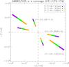 |
Fig. 1 u − v coverage of our AMBER/VLTI observations of Herschel 36. The different bandpasses are displayed in different colors. The length of each baseline is also shown. |
3. Analysis and results
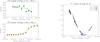 |
Fig. 2 Left: measured CPs of Herschel 36. The best-fit models are represented in green and orange lines for the H and K band. Right: Herschel 36 V2 model fitting. The panel displays the V2 for the H and K filters in black and the best-fit solution at different colors for each one of the baselines. |
We used the orbital elements calculated in Arias et al. (2010) from the spectroscopic data of Herschel 36 to estimate the apastron of component Aa and system Ab. According to the ellipse equation, the distance to the apastron is p = a(1 + e), where a is the semi-major axis and e the eccentricity of the system. Using the semi-major axis, inclination, and eccentricity from Table 3 of Arias et al. (2010), we estimated pAa + Ab for the system Aa+Ab:  (1)For the close binary Ab, we used the values from Table 2 of Arias et al. (2010) to compute pAb:
  (2)
(2)
The values of pAa + Ab and pAb at the distance of Herschel 36 thus correspond to 4 mas and 0.06 mas. In contrast to pAa + Ab, the apastron of system Ab indicates that it is below the VLTI angular resolution limit at the observed frequencies. Therefore, we fitted the calibrated V2 and CPs with a model of a binary, composed of two unresolved sources (system Ab plus component Aa). We used the software LITpro to obtain the best-fit model parameters (Tallon-Bosc et al. 2008). We emphasize that both V2 and CPs exhibit a clear cosine signature, which is typical of a binary source.
The quality of the J-band data was too low to be used in our model fitting, these data even introduced systematic residuals in the model fitting. Hence, we decided to exclude them from our analysis. This is expected because calibrating short wavelengths, such as the J band, is a difficult task in optical interferometry. It usually requires the highest performance of the instrument and good atmospheric conditions. Unfortunately, there were seeing variations, and unstable fringe lock, and low S/N of the fringe-tracking during our observations.
To circumvent these difficulties, we restricted the model fit to the data of the H and K filters. Moreover, since CPs are free of telescope-dependent phase errors induced by atmosphere and telescope vibration, they are usually more resistant to these systematic errors than the V2. Our analysis, showed that the V2 at zero baseline of the H and K bands do not reach unity. This means that an additional constant term had to be added to our binary model to achieve a good fit to the data. This over-resolved flux can be explained by an additional stellar component or extended emission (e.g., scattering halo) in the field of view (~60 mas) at a larger angular distance than the one sampled by the shortest baseline (~10 mas). To investigate these possible scenarios in more detail, additional interferometric observations with shortest baselines are required. The geometrical model of the V2 and CPs was thus fitted to the H and K filters together and to each band independently. The best-fit model parameters are reported in Table 1. The model in Fourier space, and the data are displayed in Fig. 2. Any systematic differences between model and data are within 2σ of the data uncertainties.
Our model shows an average angular separation of 1.81 ± 0.03 mas between component Aa and system Ab. Assuming that component Aa is located at the center of the frame of reference, system Ab is located at an average projected position angle of 222° ± 10.5° east of north. The best-fit flux ratio corresponds to fAb/fAa = 0.95 ± 0.12. The 1 − σ uncertainties were estimated from the standard deviations of the best-fit values of the fitting to the individual and the combined bands.
Best-fit of a binary model (system Aa + Ab) of Herschel 36 to the V2 and CPs.
Image reconstruction was performed with the package BSMEM (Buscher 1994; Lawson et al. 2004). This code uses a maximum-entropy algorithm to recover the real brightness distribution of the sources. To improve the quality of the image and reduce the sidelobes, we used the CPs and V2 of both the H and K filters at the same time for the image reconstruction. The best produced image was created after 54 iterations. The best image has a χ2 of 2.16 between the data and the final model. This image is displayed in Fig. 3 and is consistent with the best-fit geometrical model applied to the V2 and CPs. Because fAa/fAb is almost one, the photometric center is between the two components.
4. Discussion and conclusion
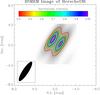 |
Fig. 3 BSMEM image of Herschel 36. Contours represent 40, 50, 60, 70, 80, 90, and 95% of the peak’s intensity. The interferometric beam (θ = λmin/2Bmax) for the data in H and K bands is of 4.50 × 1.14 mas with a position angle of 123° east of north. The northern component is the star Aa. |
We separated for the first time component Aa of Herschel 36 from the spectroscopic binary, the system Ab. Our results agree excellently well with those obtained by Arias et al. (2010). The recent statistical analysis of the brightness ratio distribution in massive multiples reported by Sana & Evans (2011) showed that close binaries typically consist of components with equal masses, while larger differences in masses can be found between components orbiting at larger angular separation. These results imply that companions at intermediate (100–1000 mas; 100–1000 AU at 1 kpc) or large spatial scales (≥1′′; ≥1000 AU at 1 kpc ) might be formed in a process independent of the processes of close spectroscopic binaries (e.g., from a different fragmented core and/or dynamical interactions; Bonnell et al. 2004).
Coplanarity of the orbits in massive multiple systems typically indicates that they were formed by a single collapse event. Hence, a complete characterization of the orbital parameters in this type of systems is mandatory for establishing useful constraints to stellar evolutionary models. In this respect, Herschel 36 is an important laboratory for determining coplanarity in massive multiples. According to Arias et al. (2010), the inclinations between the orbital planes of system Aa and Ab are related by the following relation: siniAa = 1.03siniAb. This result restricts the inclination angles to two possibilities: iAb ≈ iAa or iAb ≈ 180° − iAa.
To explore this hypothesis, we obtained a first-order approximation of the absolute orbital parameters. To determine a complete solution of the outer orbit of Herschel 36 requires some knowledge about the orbital inclination, which can only be derived accurately if at least three astrometric observations are available; unfortunately, we only have one. Therefore, some assumptions need to be made to provide an estimate of the complete orbit. We used the estimate of the inclination angles for the coplanar and non-coplanar cases (iAa ~ iAb ~70° and iAa ~ 70°, iAb ~110°, respectively) and the estimate of the masses made by Arias et al. (2010), in addition to our estimation of pAa + Ab to perform our simulations.
With these assumptions, we left the angle of the ascending node (Ω) as a free parameter in our orbital simulations. The angle of the ascending node resulted in 243° ± 12 for the coplanar and 214° ± 50 for the non-coplanar case. Figure 4 displays the orbital solutions. The large uncertainty in Ω can be explained as a result of the change in the goodness of the fit due to the measurement offset from the orbit and the projection of the ellipse onto the line that connects the measurement and model position. Figure 4 shows that components Aa and Ab of Herschel 36 appear to be very close to their periastron passage. Using the ephemeris of Arias et al. (2010), we estimated the periastrion passage for a period of 500 days of the tertiary component at the Julian date T0 = 2 456 779.5 ± 8, which is very close to the date of our AMBER observations. The small angular separation measured with our AMBER observations (~2 mas) compared with our apastron estimation agrees with this prediction.
Herschel 36 thus belongs to the increasing number of O stars that form hierarchical multiple systems, which can provide important information about the high-mass star formation scenarios. To determine whether its orbits are coplanar or not, future
astrometric near-infrared observations with the high angular interferometric resolution of AMBER and/or with the four-beam combiner PIONIER/VLTI in combination with a follow-up program of the spectroscopic solution are required.
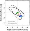 |
Fig. 4 Orbital motion of Ab (blue ellipse) around the system Aa (green ellipse). The size of the blue and green ellipses corresponds to the uncertainty of the astrometric position. The black solid ellipse corresponds to the orbital solution where both orbits are coplanar. The black dotted ellipse corresponds to the non-coplanar case. The red lines represent the periapsis, and the light-blue lines the distance from system Ab to the projected ellipses of the orbits. |
The adopted nomenclature is consistent with the denominations of the stellar components of Herschel 36 according to the Washington Double Star Catalog (WDS). Arias et al. (2010) used A, B1, and B2 for components Aa, Ab1, and Ab2, respectively.
Based on observations collected at the European Organization for Astronomical Research in the Southern Hemisphere, Chile, within observing programme 091.D-0611(A). Within the same observational programme, the ESO archive contains additional observations of Herschel 36 taken on April 2013. However, these data are not usable for scientific purposes because of technical problems with the fringe tracker FINITO.
Acknowledgments
We thank the referee for his/her useful comments. J.S.B., R.S. and A.A. acknowledge support by grants AYA2010-17631 and AYA2012-38491-CO2-02 of the Spanish Ministry of Economy and Competitiveness cofounded with FEDER founds. R.S. acknowledges support by the Ramón y Cajal programme of the Spanish Ministry of Economy and Competitiveness. J.M.A. acknowledges support by grants AYA2010-17631 and AYA2010-15081 of the Spanish Ministry of Economy and Competitiveness. RHB acknowledges financial support from FONDECYT Regular Project No. 1140076. J.I.A. acknowledges financial support from FONDECYT initiation No. 11121550. J.S.B. acknowledges support by the “JAE-PreDoc” program of the Spanish Consejo Superior de Investigaciones Científicas (CSIC), to the ESO studentship program.
References
- Arias, J. I., Barbá, R. H., Maíz Apellániz, J., Morrell, N. I., & Rubio, M. 2006, MNRAS, 366, 739 [NASA ADS] [CrossRef] [Google Scholar]
- Arias, J. I., Barbá, R. H., Gamen, R. C., et al. 2010, ApJ, 710, L30 [NASA ADS] [CrossRef] [Google Scholar]
- Bonneau, D., Clausse, J.-M., Delfosse, X., et al. 2006, A&A, 456, 789 [NASA ADS] [CrossRef] [EDP Sciences] [Google Scholar]
- Bonneau, D., Delfosse, X., Mourard, D., et al. 2011, A&A, 535, A53 [NASA ADS] [CrossRef] [EDP Sciences] [Google Scholar]
- Bonnell, I. A., Vine, S. G., & Bate, M. R. 2004, MNRAS, 349, 735 [NASA ADS] [CrossRef] [Google Scholar]
- Buscher, D. F. 1994, in Very High Angular Resolution Imaging, eds. J. G. Robertson, & W. J. Tango, IAU Proc., 158, 91 [Google Scholar]
- Chelli, A., Utrera, O. H., & Duvert, G. 2009, A&A, 502, 705 [NASA ADS] [CrossRef] [EDP Sciences] [Google Scholar]
- Goto, M., Stecklum, B., Linz, H., et al. 2006, ApJ, 649, 299 [NASA ADS] [CrossRef] [Google Scholar]
- Kraus, S., Weigelt, G., Balega, Y. Y., et al. 2009, A&A, 497, 195 [NASA ADS] [CrossRef] [EDP Sciences] [Google Scholar]
- Lawson, P. R., Cotton, W. D., Hummel, C. A., et al. 2004, New Frontiers in Stellar Interferometry, SPIE Conf. Ser., 5491, 886 [NASA ADS] [Google Scholar]
- Maíz Apellániz, J. 2010, A&A, 518, A1 [NASA ADS] [CrossRef] [EDP Sciences] [Google Scholar]
- Mason, B. D., Hartkopf, W. I., Gies, D. R., Henry, T. J., & Helsel, J. W. 2009, AJ, 137, 3358 [NASA ADS] [CrossRef] [EDP Sciences] [Google Scholar]
- Petrov, R. G., Malbet, F., Weigelt, G., et al. 2007, A&A, 464, 1 [NASA ADS] [CrossRef] [EDP Sciences] [Google Scholar]
- Sana, H., & Evans, C. J. 2011, IAU Symp., eds. C. Neiner, G. Wade, G. Meynet, & G. Peters, 272, 474 [Google Scholar]
- Sana, H., de Mink, S. E., de Koter, A., et al. 2012, Science, 337, 444 [Google Scholar]
- Sanchez-Bermudez, J., Schödel, R., Alberdi, A., et al. 2013, A&A, 554, L4 [NASA ADS] [CrossRef] [EDP Sciences] [Google Scholar]
- Sota, A., Maíz Apellániz, J., Morrell, N. I., et al. 2014, ApJS, 211, 10 [NASA ADS] [CrossRef] [Google Scholar]
- Tallon-Bosc, I., Tallon, M., Thiébaut, E., et al. 2008, SPIE Conf. Ser., 7013 [Google Scholar]
- Tatulli, E., Millour, F., Chelli, A., et al. 2007, A&A, 464, 29 [NASA ADS] [CrossRef] [EDP Sciences] [Google Scholar]
- Zinnecker, H., & Yorke, H. W. 2007, ARA&A, 45, 481 [NASA ADS] [CrossRef] [Google Scholar]
All Tables
All Figures
|
Fig. 1 u − v coverage of our AMBER/VLTI observations of Herschel 36. The different bandpasses are displayed in different colors. The length of each baseline is also shown. |
| In the text | |
|
Fig. 2 Left: measured CPs of Herschel 36. The best-fit models are represented in green and orange lines for the H and K band. Right: Herschel 36 V2 model fitting. The panel displays the V2 for the H and K filters in black and the best-fit solution at different colors for each one of the baselines. |
| In the text | |
|
Fig. 3 BSMEM image of Herschel 36. Contours represent 40, 50, 60, 70, 80, 90, and 95% of the peak’s intensity. The interferometric beam (θ = λmin/2Bmax) for the data in H and K bands is of 4.50 × 1.14 mas with a position angle of 123° east of north. The northern component is the star Aa. |
| In the text | |
|
Fig. 4 Orbital motion of Ab (blue ellipse) around the system Aa (green ellipse). The size of the blue and green ellipses corresponds to the uncertainty of the astrometric position. The black solid ellipse corresponds to the orbital solution where both orbits are coplanar. The black dotted ellipse corresponds to the non-coplanar case. The red lines represent the periapsis, and the light-blue lines the distance from system Ab to the projected ellipses of the orbits. |
| In the text | |
Current usage metrics show cumulative count of Article Views (full-text article views including HTML views, PDF and ePub downloads, according to the available data) and Abstracts Views on Vision4Press platform.
Data correspond to usage on the plateform after 2015. The current usage metrics is available 48-96 hours after online publication and is updated daily on week days.
Initial download of the metrics may take a while.