© ESO, 2014

1. Introduction and motivation

Inversion codes for the radiative transfer equation are, arguably, the best tool available to infer the physical properties of the solar atmosphere. Even though these inversion codes have been used successfully in multiple investigations (see reviews by Socas-Navarro 2001; del Toro Iniesta 2003a; Bellot Rubio 2006; Ruiz Cobo 2007), a large portion of the solar physics community still feel that they do not adequately address the questions of convergence and uniqueness. This has led many researchers to rely on simpler methods in their investigations: center-of-gravity or bisector analysis to determine the line-of-sight component of the velocity (Schlichenmaier et al. 2004; Franz & Schlichenmaier 2013), separation between I + V and I − V to determine the line-of-sight component of the magnetic field (Liu et al. 2012; Couvidat et al. 2012), separation of σ components in Stokes-I to determine the total magnetic field strength (Balthasar & Schmidt 1993; Penn & Livingston 2006), weak-field approximation to determine the magnetic field vector (Jefferies & Mickey 1991; Bello González et al. 2005), and so forth.

Nowadays, inversion codes for the radiative transfer equation are used much more often. Indeed, many data pipelines for space-borne and ground-based instruments routinely apply inversion codes for the radiative transfer equation to analyze the data. That is the case of Hinode/SP (Lites et al. 2007)¹, SDO/HMI (Borrero et al. 2011)², SOLIS/VSM (Keller et al. 2003)³. Future space-missions, such as Solar Orbiter, also plan on including inversion codes on their data-processing pipelines (Castillo Lorenzo et al. 2006; Orozco Suárez et al. 2007). The most widely used inversion codes are the so-called Milne-Eddington codes (hereafter M-E codes). Although M-E codes operate under rather restrictive assumptions about the thermodynamics of the solar plasma (Auer et al. 1977; Landolfi & Landi Degl’Innocenti 1982), they are often regarded as being able to retrieve reliable values for the magnetic and kinematic properties of the solar photosphere, and even chromoshere (Lagg 2007). However, the interpretation of M-E inferences is not straightforward, as the Milne-Eddington solution for the radiative transfer equation assumes that the magnetic field and velocity are constant with height through the solar atmosphere, which we know is not the case.

The purposes of this paper are twofold. On the one hand, we will address concerns about the convergence and uniqueness of the physical parameters retrieved by M-E inversion codes. On the other hand, we will investigate the meaning of M-E inferences in the presence of atmospheres where the magnetic field and velocity vary with height. To this end, we solve the radiative transfer equation using physical parameters derived from realistic three-dimensional non-grey magnetohydrodynamic simulations (Sect. 2), and produce synthetic Stokes profiles (Sect. 3) for two widely used magnetically sensitive neutral iron lines. The Stokes profiles are then inverted using three different inversion codes that operate under the Milne-Eddington approximation, but employ different optimization algorithms (Sect. 4). To study whether the three inversion codes converge to the same solution, their results are compared to the others’ (Sect. 5). In addition, we investigate the meaning of M-E inferences by comparing the results from the three inversion codes to the original values from the three-dimensional magneto-hydrodynamical (3D MHD) simulations (Sect. 6) in two different ways: a) assuming that the information provided by the spectral lines comes from a single optical depth in the solar photosphere; and b) employing response functions to determine exactly the layers that contribute to the formation of the selected spectral lines. Finally, we provide averaged response functions in different solar structures (granulation, sunspots, etc.) and for different physical parameters, (Sect. 7) in order to offer a quantitative explanation as to which layers the selected neutral iron lines are sensitive.

2. 3D non-grey MHD simulations

Our investigation is based on a non-grey sunspot simulation following the setup described in Rempel (2012). These are sunspot models in a domain of the size 49.152 × 49.152 × 6.144 Mm³ that were computed using grey radiative transfer and different grid resolutions. To obtain it, we restarted a non-grey simulation from the model with 16 × 16 × 12 km³ resolution in Rempel (2012) and evolved it for an additional 15 min with non-grey radiative transfer at a higher resolution of 12 × 12 × 8 km. At this resolution the domain has a size of 4096 × 4096 × 768 grid points. Figure 1 displays a 4096 × 512 subsection of the domain. The maps correspond to three physical parameters (continuum intensity, magnetic field strength B, and inclination of the magnetic field with respect to the observer’s line-of-sight γ) at a fixed optical depth. The horizontal slice contains regions that are representative of umbra, penumbra and a ~200 G plage region surrounding the spot.

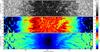Fig. 1 Overview of the magnetohydrodynamic simulations employed in this work. The upper panel shows a map of continuum intensity at λc = 630 nm, Ic(x,y), normalized to the average continuum intensity on the quiet Sun (Iqs). The middle and bottom panels show maps of magnetic field strength B(x,y) and inclination γ(x,y), respectively, at an optical depth τc = 10-2. The conversion between z and τc is described in Sect. 3. The maps in this figure have a horizontal extension of 4096 × 512 grid points or 49.152 × 6.144 Mm. The figure has been compressed along the X-axis so as to fit the entire box on the same panel.

3. Synthesis of Stokes profiles

The three dimensional magneto-hydrodynamic simulations provide data cubes for the temperature T(r), gas pressure P_g(r), density ρ(r), and velocity and magnetic field vectors v(r) and B(r). Here r refers to the position in Cartesian coordinates: r = (x,y,z). With this information, and assuming that the observer looks down into the solar atmosphere along the z-direction⁴, it is possible to solve the radiative transfer equation for polarized light (del Toro Iniesta 2003b) along the vertical z-direction for every ray path with fixed (x,y) values, $\frac{\mathit{\partial }{I}\mathrm{\left(}\mathit{z,\lambda }\mathrm{\right)}}{\mathit{\partial z}}\mathrm{=}\mathrm{𝒦̂}\mathrm{\left(}\mathit{z,\lambda }\mathrm{\right)}\mathrm{\left[}{S}\mathrm{\right(}\mathit{z,\lambda }\mathrm{)}\mathrm{-}{I}\mathrm{(}\mathit{z,\lambda }\mathrm{\left)}\mathrm{\right]}\mathit{,}$(1)where I = (I,Q,U,V)^† ( denotes transposition) is the Stokes vector, is the absorption matrix, and S the source function. The four components of the Stokes vector I_j (j = 1,...,4) are commonly referred to as Stokes parameters, and their wavelength dependence, I_j(λ), are referred to as Stokes profiles. To solve the radiative transfer equation we employ the synthesis module of the SIR code (Stokes Inversion based on Response functions; Ruiz Cobo & del Toro Iniesta 1992). The SIR code assumes Local Thermodynamic Equilibrium to compute the population of the atomic levels, and therefore the source function depends only on the local temperature S = (B [T(z),λ] ,0,0,0)^†, with B [T(z),λ] being Planck’s function for a given temperature and wavelength. The numerical integration of the radiative transfer equation is done in the optical depth scale τ_c, which is related to the z-coordinate through 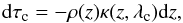$\mathrm{d}{\mathit{\tau }}_{\mathrm{c}}\mathrm{=}\mathrm{-}\mathit{\rho }\mathrm{\left(}\mathit{z}\mathrm{\right)}\mathit{\kappa }\mathrm{\left(}\mathit{z,}{\mathit{\lambda }}_{\mathrm{c}}\mathrm{\right)}\mathrm{d}\mathit{z,}$(2)where κ(z,λ_c) = κ_c(z) is the absorption coefficient per unit mass in a wavelength where there are no spectral lines (i.e., continuum). In the τ_c-scale, Eq. (1) is written as $\frac{\mathit{\partial }{I}\mathrm{\left(}{\mathit{\tau }}_{\mathrm{c}}\mathit{,\lambda }\mathrm{\right)}}{\mathit{\partial }{\mathit{\tau }}_{\mathrm{c}}}\mathrm{=}\mathrm{𝒦̂}\mathrm{\prime }\mathrm{\left(}{\mathit{\tau }}_{\mathrm{c}}\mathit{,\lambda }\mathrm{\right)}\mathrm{\left[}{I}\mathrm{\right(}{\mathit{\tau }}_{\mathrm{c}}\mathit{,\lambda }\mathrm{)}\mathrm{-}{S}\mathrm{(}{\mathit{\tau }}_{\mathrm{c}}\mathit{,\lambda }\mathrm{\left)}\mathrm{\right]}\mathit{,}$(3)where . In order to go from Eq. (1) to Eq. (3) we need to solve Eq. (2) along each ray path. To do so, we need to know ρ(z) and κ_c(z). The former is readily available through the MHD simulations. The continuum opacity κ_c(z), however, depends on several thermodynamic parameters: temperature T(z), gas pressure P_g(z), and electron pressure P_e(z). Again, the first two are provided by the MHD simulations, but the last must be computed by other means. To this end we employ an iterative technique, described in Mihalas (1970), that solves the Saha ionization equation for 83 elements plus contributions from H⁻, H⁺, and H$\begin{array}{c}\mathrm{+}\\ \mathrm{2}\end{array}$. Once P_g(z), P_e(z) and T(z) are known, we employ SIR’s opacity package (based on Wittmann 1974) to determine κ_c(z). These calculations include contributions from H, He, H⁻, He⁻, H$\begin{array}{c}\mathrm{-}\\ \mathrm{2}\end{array}$, H$\begin{array}{c}\mathrm{+}\\ \mathrm{2}\end{array}$, C, Mg, and Na, as well as Thomson scattering by free electrons and Rayleigh scattering by H, He and H₂.

In addition, a boundary condition is needed for the solution of Eq. (2). In our case we consider that τ_c = 10^-6 on the uppermost layer of the simulation box z_max = 2048 km. The conversion from the z-scale to the τ_c-scale is affected by the choice of our boundary condition only close to the uppermost layer, but it has no effect in the region where photospheric spectral lines are formed, τ_c ∈ [1,10^-4].

Although the vertical grid size of Δz = 8 km can be considered as a very good resolution from the point of view of MHD simulations, it does not necessarily guarantee that, once we convert to the optical depth scale, the step size in this new scale, Δ(log τ_c), is small enough to properly integrate the radiative transfer equation using SIR’s synthesis module (Hermitian algorithm by Bellot Rubio et al. 1998). In particular, layers where the MHD simulations show large temperature changes within a few grid points⁵ are prone to produce overshooting effects in the Hermitian algorithm. Although overshooting can be avoided by implementing better-behaved integration schemes (de la Cruz Rodríguez & Piskunov 2013), in our case, we have opted for a spline reinterpolation of the stratification in the physical parameters, after the z − τ_c conversion, into a finer grid with Δ(log τ_c) = 0.01. This ensures that the Hermitian algorithm performs adequately.

For the investigations in this paper we have synthesized two magnetically-sensitive spectral lines commonly used in spectropolarimetry. The properties of these spectral lines are summarized in Table 1. The spectral synthesis has been carried out with a wavelength sampling of 10 mÅ from −500 mÅ to + 500 mÅ around the central laboratory wavelength (λ₀) of each spectral line. The continuum between both lines has been determined considering how the wings of each line blend into that of the other line. Owing to the variations with optical depth (τ_c) in the physical quantities present in the MHD simulations, the Stokes profiles synthesized with the SIR code are, in general, asymmetric (Landolfi & Landi Degl’Innocenti 1996).

Finally, it is important to mention that, although the original simulation box contains 4096 × 4096 grid points on the XY-plane, for the tests presented in this paper we have only made use of a 4096 × 16 slice. This slice corresponds to x ∈ [1,4096] and y ∈ [248,264] in Fig. 1. As already mentioned in Sect. 2, along the x-direction this slice contains granulation, penumbra and umbra. Because the granulation is close to the sunspot it cannot be fully regarded as quiet Sun. The total number of points included in the analysis, 2¹⁶, is large enough so as to allow for statistical comparisons (see Sects. 5, 6.1, and 6.2).

4. Milne-Eddington inversion codes

Unlike the SIR code that takes into account the full dependence of the physical parameters on optical depth τ_c (see Sect. 3), Milne-Eddington (M-E) codes solve the radiative transfer equation under the Milne-Eddington approximation (Auer et al. 1977; Landolfi & Landi Degl’Innocenti 1982). This approximation assumes that many physical parameters relevant to the formation of spectral lines in solar (or stellar) atmospheres are constant or, in other words, independent of τ_c. These parameters are: η₀ (ratio between the absorption coefficient at the line-core and continuum), a (damping), Δλ_D (Doppler width of the spectral line), B (magnetic field vector, usually expressed in spherical coordinates B, γ, φ), and v_los (line-of-sight component of the velocity). In addition to this, the M-E approximation considers that the Source function varies linearly with optical depth: S(τ_c) = (S₀ + τ_cS₁,0,0,0) (see Eq. (3)). Owing to these assumptions, the solution to the polarized radiative transfer equation can be obtained analytically (Unno 1956; Rachkovsky 1962), thereby greatly improving the speed of the forward solution: I = f(M), where f(M) (see for instance Landolfi & Landi Degl’Innocenti 1982; del Toro Iniesta 2003b, Eq. (1) or Eqs. (9.44)−(9.45), respectively) is an analytic function of ${M}\mathrm{=}\mathrm{\left[}{\mathit{\eta }}_{\mathrm{0}}\mathit{,a,}\mathrm{\Delta }{\mathit{\lambda }}_{\mathrm{D}}\mathit{,}{\mathit{S}}_{\mathrm{0}}\mathit{,}{\mathit{S}}_{\mathrm{1}}\mathit{,B,\gamma ,\phi ,}{\mathit{v}}_{\mathrm{los}}\mathrm{\right]}\mathit{.}$(4)The physical parameters M enter the solution of the radiative transfer equation (Eq. (3)) in a straightforward fashion (see del Toro Iniesta 2003b, Eqs. (7.44)−(7.45)), and therefore no further attempt is made to derive any of them from the underlying microphysics. Indeed, one can surmise that the thermodynamic parameters [η₀,a,Δλ_D,S₀,S₁] could be derived from the temperature T, density ρ, electron pressure P_e, and gas pressure P_g. For instance, it could be considered that η₀ ∝ ρ, $\mathrm{\Delta }{\mathit{\lambda }}_{\mathrm{D}}\mathrm{\propto }\sqrt{\mathit{T}}$ (see del Toro Iniesta 2003b, Eqs. (6.42) and (7.40)), etc. However, in doing so, we would have to solve the Saha and Boltzmann equations numerically, and iterate to obtain the electron pressure from a given temperature and gas pressure (see Sect. 3), and so on. These numerical computations would defeat the original purpose of having an analytic solution to the radiative transfer equation (Eq. (3)). Fortunately, this does not apply to the magnetic and kinematic parameters, and therefore results for [B,γ,φ,v_los] can be readily interpreted.

The applicability M-E inversion codes is usually limited to the inversion of the observed Stokes vector in a single spectral line. Alternatively, if more lines are included in the analysis, one must take care that those spectral lines are close in wavelength and sample similar layers on the solar atmosphere. Inverting spectral lines that are far away in wavelength or formed in very different layers implies that a new set M (Eq. (4)) is needed for each line, which would multiply the number of free parameters during the inversion. This happens because each line is formed in layers characterized by very different physical conditions. A pair of lines that are close in wavelength are Fe I 6301.50 and 6302.49 Å (see Table 1). Although they do not sample exactly the same photospheric layers (Martínez González et al. 2006) they are close enough so as to allow for M-E inversions using the same set of M (Orozco Suárez et al. 2010a). Indeed, these two lines have become the lines of choice by many spectropolarimeters both on ground (Baur et al. 1981; Schmidt et al. 2003; Beck et al. 2005; Tritschler et al. 2007) and space-borne (Ichimoto et al. 2008) instruments. Other spectral lines, such as the line pair Fe I 5247.06 and 5250.22 Å, are formed even closer (Stenflo 1973; Socas-Navarro et al. 2008). However, owing to the large temperature dependence of the latter pair, we have chosen the former one for our work.

Because the physical parameters in M (Eq. (4)) are considered independent of the optical depth τ_c, the M-E solution for the radiative transfer equation is incapable of reproducing asymmetric Stokes profiles. This implies that, in general, the Milne Eddington inversion of the Stokes profiles synthesized from realistic MHD simulations (see Sect. 3) will not be able to fully reproduce those profiles. This is a well-known limitation of M-E inversion codes. However, because of their speed and simplicity (e.g., analytic solution), M-E codes have become the most widely used codes to study the solar magnetic field. Therefore, the question is whether, in spite of the drawbacks listed above, inversion codes based on the Milne-Eddington approximation are capable of reliably inferring the magnetic and kinematic properties of the solar atmosphere. Answering this question is the main purpose of this paper. We will address it in two different ways. In Sect. 5 we will study whether different M-E inversion codes agree on the magnetic and kinematic properties of the atmosphere after inverting the profiles synthesized in Sect. 3. Then, in Sect. 6 we will investigate how those results compare with the original magnetic and kinematic parameters of the MHD simulations. In the following we describe the inversion codes that will be tested in this paper.

4.1. Very Fast Inversion of the Stokes Vector inversion code: VFISV

The Very Fast Inversion of the Stokes Vector (VFISV) is a Milne-Eddington inversion code developed to analyze data from the Helioseismic and Magnetic Imager instrument onboard the Solar Dynamics Observatory satellite (Scherrer et al. 2012). Because of the unique characteristics of this instrument, VFISV is designed to invert one spectral line at a time. In addition, it assumes that the Zeeman pattern can be described under a normal Zeeman triplet (J = 1 → J = 0 transition). For these reasons, in the inversions carried out in this work, VFISV will only consider the Fe I 6302.4936 Å spectral line (see Table 1). The VFISV inversion strategy uses analytic derivatives of the Stokes vector with respect to the free parameters, and employs a combination of the Levenberg-Marquardt method (Press et al. 1986) and singular value decomposition to fit the observed profiles and retrieve the physical parameters, M (Eq. (4)), of the solar atmosphere. The initial guess for B, γ, φ, and v_los is obtained from an Artificial Neural Network that has been specifically trained, using back-propagation (Bishop 1995), for the aforementioned spectral line. In addition to this, VFISV is able to re-initialize the inversion process using random values of M if the inversion does not converge after a predetermined number of iterations. A detailed description of the code can be found in Borrero et al. (2011).

4.2. Advanced Stokes Polarimeter inversion code: ASP/HAO

The Advanced Stokes Polarimeter (ASP; Elmore et al. 1992) inversion code is a M-E inversion that evolved from early attempts (Auer et al. 1977) to invert observed Stokes profiles measured with the HAO Stokes I and Stokes II instruments. In the first modification to the code of Auer et al. (1977), Skumanich & Lites (1987) relaxed a number of approximations that were leading to non-convergent behaviour, and demonstrated the important role of scattered/stray light by fitting only the Stokes polarization profiles Q,U,V. The first systematic inversions of Stokes profiles measured across sunspots resulted from the further refinement of the ASP/HAO code (Lites & Skumanich 1990). This modification included the innovation of fitting the Stokes I profile with an added variable fraction of a stray/scattered light profile pre-determined from quiet Sun profiles. Not only was the fractional admixture of stray light determined, but the code also allows the stray light profile to shift in wavelength. Once data were available from the ASP instrument, the code had been modified to invert simultaneously two or more lines of the same multiplet (Lites et al. 1993). During the period of frequent usage of the ASP instrument (1993−2006), the ASP/HAO code was applied routinely to many data sets, and continued to see refinement. In particular, several means of initialization of the variables were developed, culminating in usage of a five-parameter genetic algorithm (Charbonneau 1995) as the default initialization. Furthermore, the code was extended to allow two magnetic components plus the non-magnetic stray/scattered light component (see, for example, Lites et al. 2002).

The ASP/HAO code also uses a Levenberg-Marquardt method for iterative fitting of the profiles, modified for accelerated convergence (Lites & Skumanich 1990). The system of linear equations is solved using stepwise regression (Jennrich 1977) rather than singular value decomposition because the latter was found to be unstable in some cases. The magnetic splitting pattern for transitions is calculated in generality under the L-S coupling assumption. The genetic algorithm is used to set initial values of B, γ, Δλ_D, η₀, and v_los. Other simpler algorithms are used to initialize the remainder of the variables. Even with only these five parameters, the genetic solution requires computational time comparable to that of the Levenberg-Marquardt procedure. For the least-squares fitting, derivatives are computed from analytical expressions. Although there is a pre-established maximum number of iteration, the code usually converges in ten or fewer (Lites & Skumanich 1990).

4.3. Helium Line Information eXtractor: HELIX⁺

The M-E code HeLIx⁺ (Lagg et al. 2004, 2009) was developed to analyze the spectral region around the He i 10 830 Å infrared triplet. This triplet often occurs in multi-lobed profiles, indicative for the complex velocity and magnetic field morphology present in an usually optically thin layer in the upper chromosphere, the formation region of this triplet (Xu et al. 2012; Sasso et al. 2011; Lagg 2007; Solanki et al. 2003). Several photospheric lines and telluric blends in the spectral vicinity are interfering with this triplet. HeLIx⁺ is optimized to treat multiple He i components, the photospheric and telluric lines simultaneously and thereby to obtain the atmospheric conditions in the photosphere and the chromosphere with a single inversion. The minimization algorithm is based on the genetic algorithm PIKAIA (Charbonneau 1995), well suited for finding the global minimum in the large parameter space resulting from this complex conditions, independent of the selection of the initial guess values. HeLIx⁺ can also take into account the Paschen-Back effect (Sasso et al. 2006) and the Hanle effect (see HAZEL code by Asensio Ramos et al. 2008) in the He i infrared triplet. However, for the application in this paper HeLIx⁺ only considers the Zeeman of the spectral lines in Table 1 under the assumption of L-S coupling. The flexible wavelength weighting scheme available in HeLIx⁺ was selected to match the scheme of VFISV and ASP/HAO.

Before proceeding with the comparison of the inversion codes described above, there are a few things that must be taken care of. The first one is to make sure that the codes are compatible as far as their synthesis modules are concerned. In other words, that for the same set of M parameters (Eq. (4)), the three codes yield the same Stokes vector I = f(M). This exercise revealed that, while ASP/HAO (Sect. 4.2) and HeLIx⁺ (Sect. 4.3) agreed almost perfectly, the VFISV code (Sect. 4.1) yielded results that differ from the others’ at the 10^-3 level. After tracking down the source of discrepancies, an error was found in VFISV when computing the imaginary part of the Voigt-Faraday function needed for the calculation of the magneto-optical effects (i.e., anti-symmetric part of the absorption matrix). It turned out that VFISV was needlessly multiplying this function by a factor of two. After correcting this bug, all three codes agreed at the 10^-6 level⁶.

The next step was to agree on the inversion set-up. In this work we are only interested in the effect of employing different minimization algorithms, thus we will not consider instrumental effects such as limited spectral/spatial sampling, photon noise, etc. These questions have already been addressed elsewhere (see for instance Orozco Suárez et al. 2010b; Borrero et al. 2007, 2011). This implies that physical parameters such as macroturbulent velocity v_mac and magnetic filling factor α_mag (commonly used in inversions) were not considered, and we only accounted for the physical parameters contained in M (Eq. (4)).

Finally, since we have not considered the effect of photon noise we give the same weights to all four Stokes parameters during the inversion: w_i = w_q = w_u = w_v = 1. These weights appear in the χ²-merit function that is being minimized during the inversion process 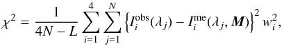${\mathit{\chi }}^{\mathrm{2}}\mathrm{=}\frac{\mathrm{1}}{\mathrm{4}\mathit{N}\mathrm{-}\mathit{L}}\sum _{\mathit{i}\mathrm{=}\mathrm{1}}^{\mathrm{4}}\sum _{\mathit{j}\mathrm{=}\mathrm{1}}^{\mathit{N}}{\mathrm{\left\{}{\mathit{I}}_{\mathit{i}}^{\mathrm{obs}}\mathrm{\right(}{\mathit{\lambda }}_{\mathit{j}}\mathrm{)}\mathrm{-}{\mathit{I}}_{\mathit{i}}^{\mathrm{me}}\mathrm{(}{\mathit{\lambda }}_{\mathit{j}}\mathit{,}{M}{\mathrm{\left)}}^{\mathrm{\right\}}}}^{\mathrm{2}}{\mathit{w}}_{\mathit{i}}^{\mathrm{2}}\mathit{,}$(5)where the index i = 1,...,4 refers to the four components of the Stokes vector (I₁ = I,I₂ = Q, etc.) and the index j = 1,...,N runs for all wavelength positions (N is the total number of wavelength positions). ${\mathit{I}}_{\mathit{i}}^{\mathrm{obs}}$ and ${\mathit{I}}_{\mathit{i}}^{\mathrm{me}}$ refer to the observed and Milne-Eddington Stokes profiles, respectively, with the latter being a function of the physical parameters in M (Eq. (4)). L in Eq. (5) refers to the total number of free parameters in M. Strictly speaking, HeLIx⁺ does not minimize χ² but instead the genetic algorithm maximizes the so-called fitness function, which has been set-up to coincide with the inverse of χ² (see Sect. 4.3).

5. Comparison between inversion codes

The analytic function f that solves the radiative transfer equation I = f(M) (Eq. (3)) is non-linear and represents, even under the simplifications of the Milne-Eddington approximation, a transcendental equation. For this reason, the inverse problem, that is, obtaining the physical parameters of the solar atmosphere from observations of the Stokes vector, cannot be analytically attained. Instead one must resort to fitting algorithms (e.g., merit function minimization; see Eq. (5)). This usually involves the use of non-linear iterative techniques that can sometimes fall into local-minima, or present uniqueness problems in the solution. To address this problem and to study to what accuracy the physical parameters of the solar atmosphere can be inferred, we will perform in this section a comparison of the solutions obtained with the three different M-E inversion codes described in Sect. 4. These codes employ rather different optimization algorithms, and therefore they are very suitable for our purpose. The comparison will be made by inverting the Stokes profiles synthesized (Sect. 3) from three-dimensional MHD simulations (Sect. 2).

Fig. 2 Comparison between the physical parameters obtained through M-E inversion codes: magnetic field strength B (top row), inclination of the magnetic field vector with respect to the observer’s line-of-sight γ (middle row), and line-of-sight velocity vlos (bottom row). The comparison between the ASP/HAO code and VFISV is displayed in the left column, while VFISV-HeLIx+and HeLIx+-ASP/HAO are compared on the middle and right columns, respectively. The color scale indicates a logarithmic density plot, where red regions contain about 3000 points from Fig. 1.

The results from the inversion of 2¹⁶ points (see Sect. 3) using VFISV, HeLIx⁺, and the ASP/HAO inversion are presented in Fig. 2 for the magnetic field strength B (top row), for the inclination of the magnetic vector with respect to the observer’s line-of-sight γ (middle row), and finally, for the line-of-sight component of the velocity v_los (bottom row). The left column in this figure compares the ASP/HAO code with VFISV, the middle column compares VFISV with HeLIx⁺, and the right column compares HeLIx⁺with the ASP/HAO code. All panels in Fig. 2 are logarithmic density plots, with red and blue colors indicating regions of high (≈10³) and low (≈1) density, respectively. In addition, each panel provides the standard deviation σ of the difference between the results of different codes for B, γ, and v_los. The best agreement in the magnetic field strength B is found between the ASP/HAO and the HeLIx⁺code, while for the inclination γ, VFISV and ASP/HAO present the most similar results. In the case of the line-of-sight velocity v_los all codes agree equally well. It is important to mention here that ASP/HAO presented a few hundred non-convergent points that have not been considered in this comparison. These points appear on the center of granules (Fig. 1). Here the ASP code yielded by design when no solution was reached zero magnetic field, B = 0, and an inclination that was either γ = 0° or γ = 180°. The suspected cause of this condition is a failure of the genetic initialization algorithm to provide a good initial guess.

In general, the three codes agree with each other at the level of σ_B ≤ 35 (Gauss), σ_γ ≤ 1.2°, and σ_v ≤ 10 m s^-1. These values are comparable or even better than those reported in Borrero et al. (2007); Orozco Suárez et al. (2010c); Fleck et al. (2011); Couvidat et al. (2012) where similar comparisons to ours were carried out but employing simpler methods, such as, center of gravity, weak-field approximation, MDI-like algorithms, etc. A direct comparison with those works cannot be done, however, because some of them add photon noise, perform spectral degradation, or analyze ideal (e.g., symmetric) profiles, etc. At any rate, our results make us confident that, despite comments to the contrary from those who are not users of inversion codes, lack of convergence does not seem to play a major role in the inferences done through M-E inversion codes. The question of uniqueness will be addressed in Sect. 6, where we will compare the physical parameters derived from the inversion to those from the numerical simuations used in the synthesis (see Sect. 3).

It is worth noting that, according to Fig. 2, the discrepancies between the inversion codes increase in those points where B ≈ 1.0 − 2.0 kG and γ ≥ 75°. Stokes profiles in this region belong to the penumbra (see Fig. 1), where the physical quantities undergo rapid changes with τ_c both in observations (Sanchez Almeida & Lites 1992) and simulations (Borrero et al. 2010). It is therefore not surprising that M-E codes, that assume that the physical quantities are constant with τ_c (see Sect. 4), present larger differences here. This effect is not seen in the line-of-sight component of the velocity v_los (Fig. 2; bottom panels) because we assume that the observer looks at the simulation box as if the sunspot was at disk center (see Sect. 3), and therefore the velocities in the penumbra, which are mainly horizontal in nature (i.e., contained in the XY-plane), contribute little to v_los.

On the other hand, close to the region where B ≥ 2.5 kG and γ ≤ 15° results seem to be particularly consistent between the three codes. Points in this region are located in the umbra (see Fig. 1). Unlike the penumbra, the umbra is characterized by smooth variations of the physical quantities with τ_c, thus resulting in a better agreement between the M-E inversion codes.

6. Comparison between inversion codes and 3D MHD simulations

6.1. At a fixed optical depth τ_c

As explained in Sect. 4, M-E inversion codes are usually restricted to single-line inversions or to line-pairs that sample very similar optical depths. Interestingly, even if a single spectral line (or several spectral lines formed very close to each other) is inverted, one must always take into account that the concept of height of formation of a spectral line is a fuzzy one (Del Toro Iniesta & Ruiz Cobo 1996; Sanchez Almeida et al. 1996). In photospheric spectral lines (e.g., absorption lines) the continuum and line-wing in Stokes I generally sample deeper layers (τ_c ≈ 1) than the line core (τ_c ≈ 10^-2 − 10^-4), but there is always a broad overlap region as a single wavelength cannot be ascribed to any particular optical depth. In addition, the aforementioned relationship only holds for Stokes I, and it can be very different for Stokes Q, U, and V. Furthermore, the photospheric layers sampled by spectral lines strongly depend on the physical parameter measured (Ruiz Cobo & del Toro Iniesta 1994). For instance, we do not sense the same layer when measuring the magnetic field or velocity at Δλ = 0 (i.e., zero-crossing) in Stokes V. All these effects make it difficult to compare the results obtained through the application of M-E inversion codes (Sect. 4) to Stokes profiles synthesized from MHD simulations (Sect. 3). While the former retrieve a single value the magnetic and kinematic parameters (B, γ, φ, v_los) at each point on the XY-plane (Fig. 1), the latter provide the full dependence on optical depth (B(τ_c), γ(τ_c), φ(τ_c), v_los(τ_c)). The problem therefore boils down to devising a strategy to compare the results from M-E inversion with those from 3D MHD simulations. Several methods have been used in the past.

One of these methods considers that the value of the physical parameters inferred from the M-E inversion must correspond to a certain height (either on an optical depth τ_c, or on a geometrical height z) in the atmosphere. To determine that height, one computes the τ_c-dependence of the standard deviation of the difference between the MHD model parameters and the constant M-E parameters. The optical depth, ${\mathit{\tau }}_{\mathrm{c}}^{\mathrm{\ast }}$, where the standard deviation is smallest is then considered to be the height where the spectral line(s) provide the most accurate information. A very similar approach is to calculate the correlation coefficient between the physical parameters from 3D MHD simulations at different heights and those from M-E inversions, and take ${\mathit{\tau }}_{\mathrm{c}}^{\mathrm{\ast }}$ as the height with the highest correlation (Kucera et al. 1998; Fleck et al. 2011). These two approaches have the disadvantage that, because ${\mathit{\tau }}_{\mathrm{c}}^{\mathrm{\ast }}$ is obtained statistically from an ensemble of very different atmospheres, whatever value is obtained for ${\mathit{\tau }}_{\mathrm{c}}^{\mathrm{\ast }}$, it does not consider that the layers where the spectral line(s) provide most information depends on the physical parameters of the atmosphere itself (Del Toro Iniesta & Ruiz Cobo 1996; Sanchez Almeida et al. 1996).

A slightly different approach is to determine, for each point on the simulation, the height at which the results from the M-E inversion and 3D MHD simulations coincide. This approach has the advantage that it allows us to study changes in the layer where the spectral line(s) provides most information (see Orozco Suárez et al. 2010c, Fig. 6). On the other hand, a shortcoming of this method is that it assumes that the error is zero, as it takes the height at which M-E inversions and numerical simulations give the same result.

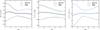Fig. 3 Mean differences (solid) and standard deviation (dashed) as a function of the optical depth τc between the original (MHD simulations) and inferred (M-E inversion) physical parameters: magnetic field strength B (left), inclination of the magnetic field with respect to the line-of-sight γ (middle), and line-of-sight component of the velocity vlos (left). Red, blue, and green colors correspond to the VFISV (Sect. 4.1), ASP/HAO (Sect. 4.2), and HeLIx+ (Sect. 4.3) inversion codes, respectively.

In this work we are interested in investigating to which accuracy M-E inversion codes can infer the magnetic and kinematic properties of the solar atmosphere, and therefore we will follow the first approach described above, that is, we determine a standard deviation between the M-E results and the MHD simulations at each optical depth (τ_c) and for each physical parameter we are interested in: B, γ, and v_los. The result of this process is presented in Fig. 3. In this figure, the solid-color lines represent the mean of the differences between the M-E inversions and the MHD simulations: ΔB (left column), Δγ (middle column), and Δv (right row). These curves allow us to see systematic differences between the inferred (through M-E inversions) and original (from MHD simulations) parameters. The dashed-color lines indicate the standard deviation between the two aforementioned values. From these plots we have determined that the optical depth, ${\mathit{\tau }}_{\mathrm{c}}^{\mathrm{\ast }}$, where the differences between the inferred vales and the original ones are smallest, are: $\log {\mathit{\tau }}_{\mathrm{c}}^{\mathrm{\ast }}\mathrm{\approx }\mathrm{-}\mathrm{1.4}$ for B, $\log {\mathit{\tau }}_{\mathrm{c}}^{\mathrm{\ast }}\mathrm{\approx }\mathrm{-}\mathrm{1.7}$ for γ, and $\log {\mathit{\tau }}_{\mathrm{c}}^{\mathrm{\ast }}\mathrm{\approx }\mathrm{-}\mathrm{1.0}$ for v_los. The fact that ${\mathit{\tau }}_{\mathrm{c}}^{\mathrm{\ast }}$ is different for each physical parameter strongly supports the idea that a spectral line provides information about different photospheric layers depending on the physical parameter measured (Ruiz Cobo & del Toro Iniesta 1994).

Figure 4 presents similar scatter-density plots to those in Fig. 2 but comparing the results obtained through the M-E inversions with those from the 3D MHD numerical simulations at the heights of maximum information, ${\mathit{\tau }}_{\mathrm{c}}^{\mathrm{\ast }}$, that have just been determined. From this figure we obtained the following errors: σ_B< 130 G (magnetic field strength), σ_γ< 5° (inclination of the magnetic field vector with respect to the observer’s line of sight), σ_v< 320 m s^-1 (line-of-sight component of the velocity). As previously observed and explained (Sect. 5; Fig. 2) the errors increase in the penumbra, but decrease in the umbra.

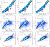Fig. 4 Scatter-density plots of the physical parameters inferred through M-E inversion codes (vertical axis) and the original values from the 3D MHD numerical simulations (horizontal axis). The values from the simulations are taken at $\log {\mathit{\tau }}_{\mathrm{c}}^{\mathrm{\ast }}\mathrm{=}\mathrm{-}\mathrm{1.4}\mathit{,}\mathrm{-}\mathrm{1.7}\mathit{,}\mathrm{-}\mathrm{1.0}$ for B (top rows), γ (middle rows), and vlos (bottom rows), respectively. Left column corresponds to VFISV, middle one to ASP/HAO, and right one to HeLIx+. Standard deviations σ are also indicated for each physical parameter and for each inversion code.

6.2. Using response functions

As mentioned in Sect. 6.1, it is not possible to assign a single optical depth to the measurement of a particular physical parameter, even if the measurement is done at a single wavelength. The proper way to compare the τ_c-independent results from M-E inversions with the τ_c-dependent values from MHD simulations, is to compare (at every point in the XY-plane in Fig. 1) the former with an average of the latter. We define this average as $\begin{array}{c}\mathrm{􏽥}\\ {\mathit{X}}^{\mathrm{mhd}}\end{array}\mathrm{=}\underset{\mathrm{0}}{\overset{\mathrm{\infty }}{\mathrm{\int }}}{\mathit{w}}_{\mathit{x}}\mathrm{\left(}{\mathit{\tau }}_{\mathrm{c}}\mathrm{\right)}{\mathit{X}}^{\mathrm{mhd}}\mathrm{\left(}{\mathit{\tau }}_{\mathrm{c}}\mathrm{\right)}\mathrm{d}{\mathit{\tau }}_{\mathrm{c}}\mathit{,}$(6)where w_x(τ_c) is a weighting function that conveys the information as to which atmospheric layers the spectral line(s) is sensitive to. We emphasize that w_x(τ_c) is different for each physical parameter X (e.g., X = B, X = γ, and X = v_los), and for each (x,y) point on the simulation. In this sense, w_x(τ_c) can be understood as a sensitivity kernel, akin to those employed in Helioseismology (see Birch & Kosovichev 2000, and references therein). In this work, we consider the following weighting function, 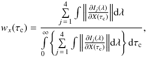${\mathit{w}}_{\mathit{x}}\mathrm{\left(}{\mathit{\tau }}_{\mathrm{c}}\mathrm{\right)}\mathrm{=}\frac{\sum _{\mathit{j}\hspace{0.17em}\mathrm{=}\hspace{0.17em}\mathrm{1}}^{\mathrm{4}}\begin{array}{c}\mathrm{\int }\end{array}\begin{array}{c}\mathrm{\parallel }\\ \mathrm{\parallel }\\ \mathrm{\parallel }\\ \mathrm{\parallel }\end{array}{}^{}\frac{\mathit{\partial }{\mathit{I}}_{\mathit{j}}\mathrm{\left(}\mathit{\lambda }\mathrm{\right)}}{\mathit{\partial X}\mathrm{\left(}{\mathit{\tau }}_{\mathrm{c}}\mathrm{\right)}}\begin{array}{c}\mathrm{\parallel }\\ \mathrm{\parallel }\\ \mathrm{\parallel }\\ \mathrm{\parallel }\end{array}{}^{}\mathrm{d}\mathit{\lambda }}{\underset{\mathrm{0}}{\overset{\mathrm{\infty }}{\mathrm{\int }}}\left\{\sum _{\mathit{j}\hspace{0.17em}\mathrm{=}\hspace{0.17em}\mathrm{1}}^{\mathrm{4}}\begin{array}{c}\mathrm{\int }\end{array}\begin{array}{c}\mathrm{\parallel }\\ \mathrm{\parallel }\\ \mathrm{\parallel }\\ \mathrm{\parallel }\end{array}{}^{}\frac{\mathit{\partial }{\mathit{I}}_{\mathit{j}}\mathrm{\left(}\mathit{\lambda }\mathrm{\right)}}{\mathit{\partial X}\mathrm{\left(}{\mathit{\tau }}_{\mathrm{c}}\mathrm{\right)}}\begin{array}{c}\mathrm{\parallel }\\ \mathrm{\parallel }\\ \mathrm{\parallel }\\ \mathrm{\parallel }\end{array}{}^{}\mathrm{d}\mathit{\lambda }\right\}\mathrm{d}{\mathit{\tau }}_{\mathrm{c}}}\mathit{,}$(7)where index j runs for all four components of the Stokes vector (see Sect. 3). The partial derivatives of I_j (Stokes profiles) with respect to X are the so-called Response Functions (Beckers & Milkey 1975; Caccin et al. 1977; Landi Degl’Innocenti & Landi Degl’Innocenti 1977), and can be interpreted as the changes in the j-component of the Stokes vector I(λ) when a small perturbation is added at some optical depth τ_c. The weighting functions for HeLIx⁺and ASP/HAO codes are obtained through a wavelength integral that includes both spectral lines in Table 1. However, for VFISV, the wavelength integral includes only the second spectral line in this table (see Sect. 4.1). We note that the denominator in Eq. (7) ensures that w_x(τ_c) is normalized to unity.

The absolute value is taken inside the integral in Eq. (7) because the response function can be positive at some wavelengths but negative at others. If we perform a straight integral summation, the contribution at different wavelengths might cancel out. This situation is not desirable because a negative response is a response after all, and still indicates that the spectral line is sensitive at that wavelength for a particular X(τ_c) perturbation.

To perform the comparison between M-E inversion codes and MHD simulations according to Eqs. (6) and (7), we need to calculate the response functions of the Stokes vector with respect to B, γ, and v_los as a function of wavelength, λ, and optical depth, τ_c, for the spectral lines in Table 1. This was done, for every point on the XY-plane in Fig. 1, employing the SIR inversion code (Ruiz Cobo & del Toro Iniesta 1992).

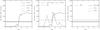Fig. 5 Left panel: original stratification of the magnetic field strength as a function of optical depth from the 3D MHD simulation Bmhd(τc) (solid-black line) for a particular point of the simulation domain (x = 500,y = 250; see Fig. 1). The color lines represent the results from the Milne-Eddington inversion of the Stokes profiles synthesized from the MHD simulation. Middle panel: here the solid-black is the same as on the left panel, Bmhd(τc); the dashed-black line represents the weighting function wB(τc) employed to calculated the weighted average $\begin{array}{c}{\mathrm{􏽥}}_{}\\ {\mathit{B}}^{\mathrm{mhd}}\end{array}$ (dashed-dotted black line) according to Eq. (6). Right panel: comparison between the weighted average value of the magnetic field $\begin{array}{c}{\mathrm{􏽥}}_{}\\ {\mathit{B}}^{\mathrm{mhd}}\end{array}$ (dashed-dotted black line) from the numerical simulations with the magnetic field obtained from the M-E inversions (solid-color lines).

Figure 5 illustrates an example of the process we have just described. On the leftmost panel we plot (solid-black line) the dependence of the magnetic field strength on the optical depth given by the MHD simulations, B^mhd(τ_c), for point (x = 500,y = 250) in Fig. 1. We also plot (solid-color lines) the results from the inversion with the three different M-E inversion codes described in Sect. 4. Due to the assumptions of the Milne-Eddington model, the color lines are constant with τ_c. The question we posed earlier in this section was about comparing the results from the M-E inversions with B^mhd(τ_c). In Sect. 6.1 we compared with ${\mathit{B}}^{\mathrm{mhd}}\mathrm{(}\log {\mathit{\tau }}_{\mathrm{c}}^{\mathrm{\ast }}\mathrm{=}\mathrm{-}\mathrm{1.4}\mathrm{)}$. However, in this section we employ the weighting function, w_B(τ_c), showcased in the middle panel of Fig. 5 (dashed-black line). For simplicity, in this example we consider that w_B(τ_c) is the same for the three M-E inversion codes tested, even though we know they are not because VFISV includes only one spectral line in the wavelength integral in Eq. (7). With it, a weighted average of B^mhd(τ_c) is then calculated according to Eq. (6), resulting in $\begin{array}{c}{\mathrm{􏽥}}_{}\\ {\mathit{B}}^{\mathrm{mhd}}\end{array}$ (dashed-dotted line in middle panel). This is the actual value that is then compared to the results from the Milne-Eddington inversions (right panel in Fig. 5). The process must then be repeated for γ, and v_los and for all 2¹⁶ points in the simulation. For each case, a new weighting function must be calculated because the sensitivity of the spectral line depends on both the physical parameter measured and the properties of the atmosphere where it is measured.

The results of the comparison employing response functions are presented in Fig. 6. This figure is analogous to Figs. 2 and 4. When compared to Fig. 4, we observe that employing proper kernels to determine the heights at which the spectral lines are sensitive, significantly increases the agreement between MHD simulations and the M-E inversions: σ_B< 90 G, σ_γ< 3°, the line-of-sight component of the velocity σ_v< 90 m s^-1. These results strongly support the idea that M-E inversions provide an average of the physical parameters across the region in which the spectral lines are formed. Although not the first time this fact is pointed out (see e.g., Westendorp Plaza et al. 1998, Sect. 3.1), our work here certainly provides the most exhaustive demonstration to date, insofar as we have employed realistic numerical simulations of sunspots (Sect. 2) to produce a large number of synthetic profiles (Sect. 3) that were subsequently analyzed using three different M-E inversion codes (Sect. 4). Moreover, the results presented in this section also ward off criticism about the lack of uniqueness in the inversion results, as we have now demonstrated, these are very similar to the original values from the MHD simulations.

Last but not least, we have also followed the more rigorous approach, described in Sanchez Almeida et al. (1996), to determine the weighting function w_x through the use of generalized Response Functions. The advantage of these functions is that they are positively defined, and therefore, there is no need to introduce the (somewhat artificial) absolute value in Eq. (7). In particular, the term ∂g/∂I_i in Eq. (14) in Sanchez Almeida et al. (1996) should become negative whenever the response function is also negative, so that their product (see Eq. (8) in the cited paper) remains positive (Sánchez Almeida, priv. comm.). Interestingly, after we tested this method using the stratification from the MHD simulations we observed that this is often not the case. This forced us to, again, introduce an absolute value in this more rigorous formulation of the problem⁷. We suspect that the inconsistency arises from the large variations with optical depth present in the MHD simulations (see e.g., solid-black line in Fig. 5), that can break down the assumption of linear perturbations implicit in our Eq. (6) (see also Eq. (10) in Sanchez Almeida et al. 1996). We tried to confirm this point by evaluating the physical parameters in the simulations in a grid with Δlog τ_c = 10^-3 instead of Δlog τ_c = 10^-2 (see Sect. 3) but to no avail. For these reasons we decided not to pursue this strategy further.

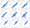Fig. 6 Same as Fig. 4 but comparing the results from the M-E inversions with the weighted averages of the MHD simulations $\begin{array}{c}{\mathrm{􏽥}}_{}\\ {\mathit{B}}^{\mathrm{mhd}}\end{array}$, $\stackrel{}{{{\mathit{\gamma }}^{\mathrm{mhd}}}^{\mathrm{􏽥}}}$, $\stackrel{}{{{\mathit{v}}_{\mathrm{los}}^{\mathrm{mhd}}}^{\mathrm{􏽥}}}$ instead of the values at some fixed optical depth value ${\mathit{\tau }}_{\mathrm{c}}^{\mathrm{\ast }}$.

7. Optical depths for the formation of the Fe I line pair at 630 nm

In Sect. 6.2 we demonstrated that, after taking into account the atmospheric layers sampled by the spectral lines in Table 1 when measuring B, γ, and v_los, the agreement between the M-E inversions and MHD simulations improved greatly. For instance, the standard deviations in Fig. 6 are up to a factor of 2−3 smaller than those in Fig. 4. This illustrates the need for a proper account of the layers sensed by spectral lines when measuring different physical parameters. In an attempt to provide such account we present, in Fig. 7, the average of the weighting functions $\begin{array}{c}{}_{\mathrm{􏽥}}\\ {\mathit{w}}_{\mathit{x}}\end{array}\mathrm{\left(}{\mathit{\tau }}_{\mathrm{c}}\mathrm{\right)}$ employed in the previous section for B (left column), γ (middle column), and v_los (right column) in several solar structures: granules (first row), intergranules (second row), penumbra (third row) and umbra (fourth row). These averages were determined by selecting points in the simulations (Fig. 1) that identify these structures, and then averaging the individual weighting functions from each of those pixels.

The dashed-vertical lines in Fig. 7 represent the median of the distribution. This line indicates, by definition, that the spectral lines employed in this work are equally responsive to the layers above it than to the layers beneath it. The shaded areas in each panel include the layers where the sum of the sorted (from highest to lowest) values of $\begin{array}{c}{\mathrm{􏽥}}_{}\\ {\mathit{w}}_{\mathit{x}}\end{array}$ adds up to 90% of the total area under $\begin{array}{c}{}_{\mathrm{􏽥}}\\ {\mathit{w}}_{\mathit{x}}\end{array}\mathrm{\left(}{\mathit{\tau }}_{\mathrm{c}}\mathrm{\right)}$. These regions can be then considered as the regions where most of the sensitivity of the spectral lines comes from.

From this figure we infer that, on average, the response of the spectral lines to variations in B, γ, and v_los is restricted to a narrower region (log τ_c ∈ [0, −2.5]) in the penumbra than in granules and intergranules (log τ_c ∈ [0, −3.5]). The response in the umbra is spread mostly over a region between log τ_c ∈ [0, −3.0]. In some cases, in particular in the umbra and penumbra, $\begin{array}{c}{}_{\mathrm{􏽥}}\\ {\mathit{w}}_{\mathit{x}}\end{array}\mathrm{\left(}{\mathit{\tau }}_{\mathrm{c}}\mathrm{\right)}$ presents a strong narrow peak that could be used to argue in favor of the idea that the spectral lines are formed at some particular height. As discussed in Sect. 6.2 and demonstrated here (see also Sanchez Almeida et al. 1996; Del Toro Iniesta & Ruiz Cobo 1996) this interpretation is, however, misleading. Particularly interesting is the case of granules and intergranules (top two rows in Fig. 7), where layers spread over wide optical depth regions are equally sensitive to variations in the physical parameters. An extreme example of this is the case of the granular response to variations in v_los (top-middle panel in Fig. 7), where $\begin{array}{c}{}_{\mathrm{􏽥}}\\ {\mathit{w}}_{\mathit{v}}\end{array}\mathrm{\left(}{\mathit{\tau }}_{\mathrm{c}}\mathrm{\right)}$ presents a bimodal distribution. Here, we distinguish two regions of large sensitivity, log τ_c ∈ [0, −1] and log τ_c ∈ [−2, −4], but very little response to variations in v_los in the layers located between these two regions: log τ_c ∈ [−1, −2].

The averaged weighting functions $\begin{array}{c}{}_{\mathrm{􏽥}}\\ {\mathit{w}}_{\mathit{x}}\end{array}\mathrm{\left(}{\mathit{\tau }}_{\mathrm{c}}\mathrm{\right)}$ from Fig. 7 can be useful to interpret the inferences from M-E inversion codes, as they can help assign (to first-order) where in the photosphere the measurement is done. Here we note that the response functions depend on the physical parameters of the atmosphere (see Sect. 6.2). For this reason we have tried to average $\begin{array}{c}{}_{\mathrm{􏽥}}\\ {\mathit{w}}_{\mathit{x}}\end{array}\mathrm{\left(}{\mathit{\tau }}_{\mathrm{c}}\mathrm{\right)}$ from individual pixels that correspond to similar solar structures so that the physical parameters, and thus also the response functions, are similar. However, this is never strictly the case (e.g., the physical conditions are not the same at the center of a granule as at the edge) and consequently the interpretation of $\begin{array}{c}{}_{\mathrm{􏽥}}\\ {\mathit{w}}_{\mathit{x}}\end{array}\mathrm{\left(}{\mathit{\tau }}_{\mathrm{c}}\mathrm{\right)}$ should be done with care. We emphasize, however, that employing the functions $\begin{array}{c}{}_{\mathrm{􏽥}}\\ {\mathit{w}}_{\mathit{x}}\end{array}\mathrm{\left(}{\mathit{\tau }}_{\mathrm{c}}\mathrm{\right)}$ from Fig. 7 is clearly preferable to assigning a single optical depth to the measurement (see Sect. 6.1 and references therein).

Fig. 7 Averaged weighting functions $\begin{array}{c}{\mathrm{􏽥}}_{}\\ {\mathit{w}}_{\mathit{x}}\end{array}$ for different physical parameters and different solar structures. From left to right: B, γ, and vlos. From top to bottom: granules, intergranules, penumbra, and umbra. Each panel indicates the number of points from Fig. 1 employed in the average. The vertical dashed lines correspond to the median of each distribution. Shaded areas encompass the regions of highest sensitivity (see text for details).

8. Summary and conclusions

Milne-Eddington (M-E) inversion codes for the radiative transfer equation are the most widely used tools to infer the magnetic field vector from observations of the polarization signals in photospheric and chromospheric spectral lines. A comprehensive comparison between the different M-E codes available to the solar physics community is still missing, and so is a physical interpretation of their inferences. To address these questions we have carried out a comparison between three of those codes: VFISV, ASP/HAO, and HeLIx⁺. The three M-E codes have been used to invert synthetic Stokes profiles that were previously obtained from realistic non-grey 3D MHD simulations.

Our results indicate that the three tested M-E codes agree within approximately 30 Gauss in the determination of the magnetic field strength B, within 1° in the determination of the inclination of the magnetic field γ, and finally, within 100 m s^-1in the determination of the line-of-sight component of the velocity v_los. Compared with the 3D MHD numerical simulations at a fixed optical depth, M-E codes retrieve the correct values within 130 Gauss, 5°, and 320 m s^-1 in B, γ, and v_los respectively. We have argued, however, that comparisons at a fixed optical depth or geometrical height are misleading because they do not consider that the Stokes parameters convey information about a wide range of optical depths, and these ranges vary with the physical parameter being inferred. Moreover, the atmosphere itself plays a role, and therefore the same physical parameter is measured in different atmospheric layers if we look, for instance, at granules and intergranules.

To properly account for all the aforementioned effects we have employed the response functions of the Stokes vector to the different physical parameters to determine the exact range of optical depths that should be employed in the comparison between 3D MHD numerical simulations and the inferences made by M-E inversion codes. Once this is accounted for, the agreement between the numerical simulations and M-E codes improves: 90 Gauss in B, 3° in γ, and 90 m s^-1 in v_los. Finally, we have provided the approximate optical depth regions that convey information, in the Fe I line pair at 630 nm, about the magnetic field strength, inclination and line-of-sight velocity in granules, intergranules, penumbral and umbral regions.

Acknowledgments

This research has been carried out in the frame of the two meetings held in February 2010 and December 2012 at the International Space Science Institute (ISSI) in Bern (Switzerland) as part of the International Working group Extracting Information from spectropolarimetric observations: comparison of inversion codes. We are particularly grateful to Dr. Maurizio Falanga, Andrea Fischer and Jennifer Zaugg for their hospitality and help organizing the meetings. Discussions with Drs. Michiel van Noort, Arturo López, Andrés Asensio Ramos, Héctor Socas-Navarro, and Nikola Vitas are also greatfully acknowledged. R.R. acknowledges financial support by DFG grant RE 3282/1-1. This work has made use of the NASA Astrophysical Data System. The National Center for Atmospheric Research is sponsored by the National Science Foundation. This investigation is based on work supported by the National Science Foundation under Grant numbers 0711134, 0933959, 1041709, and 1041710 and the University of Tennessee through the use of the Kraken computing resource at the National Institute for Computational Sciences (http://www.nics.tennessee.edu).

References

All Tables

All Figures

Fig. 1 Overview of the magnetohydrodynamic simulations employed in this work. The upper panel shows a map of continuum intensity at λc = 630 nm, Ic(x,y), normalized to the average continuum intensity on the quiet Sun (Iqs). The middle and bottom panels show maps of magnetic field strength B(x,y) and inclination γ(x,y), respectively, at an optical depth τc = 10-2. The conversion between z and τc is described in Sect. 3. The maps in this figure have a horizontal extension of 4096 × 512 grid points or 49.152 × 6.144 Mm. The figure has been compressed along the X-axis so as to fit the entire box on the same panel.

In the text

Fig. 2 Comparison between the physical parameters obtained through M-E inversion codes: magnetic field strength B (top row), inclination of the magnetic field vector with respect to the observer’s line-of-sight γ (middle row), and line-of-sight velocity vlos (bottom row). The comparison between the ASP/HAO code and VFISV is displayed in the left column, while VFISV-HeLIx+and HeLIx+-ASP/HAO are compared on the middle and right columns, respectively. The color scale indicates a logarithmic density plot, where red regions contain about 3000 points from Fig. 1.

In the text

Fig. 3 Mean differences (solid) and standard deviation (dashed) as a function of the optical depth τc between the original (MHD simulations) and inferred (M-E inversion) physical parameters: magnetic field strength B (left), inclination of the magnetic field with respect to the line-of-sight γ (middle), and line-of-sight component of the velocity vlos (left). Red, blue, and green colors correspond to the VFISV (Sect. 4.1), ASP/HAO (Sect. 4.2), and HeLIx+ (Sect. 4.3) inversion codes, respectively.

In the text

Fig. 4 Scatter-density plots of the physical parameters inferred through M-E inversion codes (vertical axis) and the original values from the 3D MHD numerical simulations (horizontal axis). The values from the simulations are taken at $\log {\mathit{\tau }}_{\mathrm{c}}^{\mathrm{\ast }}\mathrm{=}\mathrm{-}\mathrm{1.4}\mathit{,}\mathrm{-}\mathrm{1.7}\mathit{,}\mathrm{-}\mathrm{1.0}$ for B (top rows), γ (middle rows), and vlos (bottom rows), respectively. Left column corresponds to VFISV, middle one to ASP/HAO, and right one to HeLIx+. Standard deviations σ are also indicated for each physical parameter and for each inversion code.

In the text

Fig. 5 Left panel: original stratification of the magnetic field strength as a function of optical depth from the 3D MHD simulation Bmhd(τc) (solid-black line) for a particular point of the simulation domain (x = 500,y = 250; see Fig. 1). The color lines represent the results from the Milne-Eddington inversion of the Stokes profiles synthesized from the MHD simulation. Middle panel: here the solid-black is the same as on the left panel, Bmhd(τc); the dashed-black line represents the weighting function wB(τc) employed to calculated the weighted average $\begin{array}{c}{\mathrm{􏽥}}_{}\\ {\mathit{B}}^{\mathrm{mhd}}\end{array}$ (dashed-dotted black line) according to Eq. (6). Right panel: comparison between the weighted average value of the magnetic field $\begin{array}{c}{\mathrm{􏽥}}_{}\\ {\mathit{B}}^{\mathrm{mhd}}\end{array}$ (dashed-dotted black line) from the numerical simulations with the magnetic field obtained from the M-E inversions (solid-color lines).

In the text

Fig. 6 Same as Fig. 4 but comparing the results from the M-E inversions with the weighted averages of the MHD simulations $\begin{array}{c}{\mathrm{􏽥}}_{}\\ {\mathit{B}}^{\mathrm{mhd}}\end{array}$, $\stackrel{}{{{\mathit{\gamma }}^{\mathrm{mhd}}}^{\mathrm{􏽥}}}$, $\stackrel{}{{{\mathit{v}}_{\mathrm{los}}^{\mathrm{mhd}}}^{\mathrm{􏽥}}}$ instead of the values at some fixed optical depth value ${\mathit{\tau }}_{\mathrm{c}}^{\mathrm{\ast }}$.

In the text

Fig. 7 Averaged weighting functions $\begin{array}{c}{\mathrm{􏽥}}_{}\\ {\mathit{w}}_{\mathit{x}}\end{array}$ for different physical parameters and different solar structures. From left to right: B, γ, and vlos. From top to bottom: granules, intergranules, penumbra, and umbra. Each panel indicates the number of points from Fig. 1 employed in the average. The vertical dashed lines correspond to the median of each distribution. Shaded areas encompass the regions of highest sensitivity (see text for details).

In the text

References

- Anstee, S. D., & O’Mara, B. J. 1995, MNRAS, 276, 859 [NASA ADS] [CrossRef] [Google Scholar]
- Asensio Ramos, A., Trujillo Bueno, J., & Landi Degl’Innocenti, E. 2008, ApJ, 683, 542 [NASA ADS] [CrossRef] [Google Scholar]
- Auer, L. H., House, L. L., & Heasley, J. N. 1977, Sol. Phys., 55, 47 [NASA ADS] [CrossRef] [Google Scholar]
- Balthasar, H., & Schmidt, W. 1993, A&A, 279, 243 [NASA ADS] [Google Scholar]
- Bard, A., Kock, A., & Kock, M. 1991, A&A, 248, 315 [NASA ADS] [Google Scholar]
- Baur, T. G., Elmore, D. E., Lee, R. H., Querfeld, C. W., & Rogers, S. R. 1981, Sol. Phys., 70, 395 [Google Scholar]
- Beck, C., Schmidt, W., Kentischer, T., & Elmore, D. 2005, A&A, 437, 1159 [NASA ADS] [CrossRef] [EDP Sciences] [Google Scholar]
- Beckers, J. M., & Milkey, R. W. 1975, Sol. Phys., 43, 289 [NASA ADS] [CrossRef] [Google Scholar]
- Bello González, N., Okunev, O. V., Domínguez Cerdeña, I., Kneer, F., & Puschmann, K. G. 2005, A&A, 434, 317 [NASA ADS] [CrossRef] [EDP Sciences] [Google Scholar]
- Bellot Rubio, L. R. 2006, in ASP Conf. Ser. 358, eds. R. Casini, & B. W. Lites, 107 [Google Scholar]
- Bellot Rubio, L. R., Ruiz Cobo, B., & Collados, M. 1998, ApJ, 506, 805 [NASA ADS] [CrossRef] [Google Scholar]
- Birch, A. C., & Kosovichev, A. G. 2000, Sol. Phys., 192, 193 [NASA ADS] [CrossRef] [Google Scholar]
- Bishop, C. M. 1995, Neural Networks for Pattern Recognition (Oxford University Press) [Google Scholar]
- Borrero, J. M., Tomczyk, S., Norton, A., et al. 2007, Sol. Phys., 240, 177 [NASA ADS] [CrossRef] [Google Scholar]
- Borrero, J. M., Rempel, M., & Solanki, S. K. 2010, Astron. Nachr., 331, 567 [NASA ADS] [CrossRef] [Google Scholar]
- Borrero, J. M., Tomczyk, S., Kubo, M., et al. 2011, Sol. Phys., 273, 267 [Google Scholar]
- Caccin, B., Gomez, M. T., Marmolino, C., & Severino, G. 1977, A&A, 54, 227 [NASA ADS] [Google Scholar]
- Castillo Lorenzo, J. L., Orozco Suárez, D., Bellot Rubio, L. R., Jiménez, L., & Del Toro Iniesta, J. C. 2006, in ASP Conf. Ser. 358, eds. R. Casini, & B. W. Lites, 177 [Google Scholar]
- Centeno, R., Schou, J., Hayashi, K., et al. 2014, Sol. Phys. 289, 3531 [Google Scholar]
- Charbonneau, P. 1995, ApJS, 101, 309 [NASA ADS] [CrossRef] [Google Scholar]
- Couvidat, S., Rajaguru, S. P., Wachter, R., et al. 2012, Sol. Phys., 278, 217 [NASA ADS] [CrossRef] [Google Scholar]
- de la Cruz Rodríguez, J., & Piskunov, N. 2013, ApJ, 764, 33 [NASA ADS] [CrossRef] [Google Scholar]
- del Toro Iniesta, J. C. 2003a, Astron. Nachr., 324, 383 [NASA ADS] [CrossRef] [Google Scholar]
- del Toro Iniesta, J. C. 2003b, Introduction to Spectropolarimetry (Cambridge University Press) [Google Scholar]
- Del Toro Iniesta, J. C., & Ruiz Cobo, B. 1996, Sol. Phys., 164, 169 [NASA ADS] [CrossRef] [Google Scholar]
- Elmore, D. F., Lites, B. W., Tomczyk, S., et al. 1992, in Polarization Analysis and Measurement, eds. D. H. Goldstein, & R. A. Chipman, SPIE Conf. Ser., 1746, 22 [Google Scholar]
- Fleck, B., Couvidat, S., & Straus, T. 2011, Sol. Phys., 271, 27 [NASA ADS] [CrossRef] [Google Scholar]
- Franz, M., & Schlichenmaier, R. 2013, A&A, 550, A97 [NASA ADS] [CrossRef] [EDP Sciences] [Google Scholar]
- Ichimoto, K., Lites, B., Elmore, D., et al. 2008, Sol. Phys., 249, 233 [NASA ADS] [CrossRef] [Google Scholar]
- Jefferies, J. T., & Mickey, D. L. 1991, ApJ, 372, 694 [NASA ADS] [CrossRef] [Google Scholar]
- Jennrich, R. 1977, Stepwise Regression [Google Scholar]
- Keller, C. U., Harvey, J. W., & Solis Team 2003, in Solar Polarization, eds. J. Trujillo-Bueno, & J. Sanchez Almeida, ASP Conf. Ser., 307, 13 [Google Scholar]
- Kucera, A., Balthasar, H., Rybak, J., & Woehl, H. 1998, A&A, 332, 1069 [NASA ADS] [Google Scholar]
- Lagg, A. 2007, Adv. Space Res., 39, 1734 [Google Scholar]
- Lagg, A., Woch, J., Krupp, N., & Solanki, S. K. 2004, A&A, 414, 1109 [NASA ADS] [CrossRef] [EDP Sciences] [Google Scholar]
- Lagg, A., Ishikawa, R., Merenda, L., et al. 2009, in The Second Hinode Science Meeting: Beyond Discovery-Toward Understanding, eds. B. Lites, M. Cheung, T. Magara, J. Mariska, & K. Reeves, ASP Conf. Ser., 415, 327 [Google Scholar]
- Landi Degl’Innocenti, E., & Landi Degl’Innocenti, M. 1977, A&A, 56, 111 [NASA ADS] [Google Scholar]
- Landolfi, M., & Landi Degl’Innocenti, E. 1982, Sol. Phys., 78, 355 [NASA ADS] [CrossRef] [Google Scholar]
- Landolfi, M., & Landi Degl’Innocenti, E. 1996, Sol. Phys., 164, 191 [NASA ADS] [CrossRef] [Google Scholar]
- Lites, B. W., & Skumanich, A. 1990, ApJ, 348, 747 [NASA ADS] [CrossRef] [Google Scholar]
- Lites, B. W., Elmore, D. F., Seagraves, P., & Skumanich, A. P. 1993, ApJ, 418, 928 [NASA ADS] [CrossRef] [Google Scholar]
- Lites, B. W., Socas-Navarro, H., Skumanich, A., & Shimizu, T. 2002, ApJ, 575, 1131 [NASA ADS] [CrossRef] [Google Scholar]
- Lites, B., Casini, R., Garcia, J., & Socas-Navarro, H. 2007, Mem. Soc. Astron. It., 78, 148 [NASA ADS] [Google Scholar]
- Liu, Y., Hoeksema, J. T., Scherrer, P. H., et al. 2012, Sol. Phys., 279, 295 [Google Scholar]
- Martínez González, M. J., Collados, M., & Ruiz Cobo, B. 2006, A&A, 456, 1159 [NASA ADS] [CrossRef] [EDP Sciences] [Google Scholar]
- Mihalas, D. 1970, Stellar atmospheres (San Francisco: Freeman) [Google Scholar]
- Nave, G., Johansson, S., Learner, R. C. M., Thorne, A. P., & Brault, J. W. 1994, ApJS, 94, 221 [NASA ADS] [CrossRef] [Google Scholar]
- Orozco Suárez, D., Bellot Rubio, L. R., Vargas, S., et al. 2007, in ESA SP, 641 [Google Scholar]
- Orozco Suárez, D., Bellot Rubio, L. R., & Del Toro Iniesta, J. C. 2010a, A&A, 518, A3 [NASA ADS] [CrossRef] [EDP Sciences] [Google Scholar]
- Orozco Suárez, D., Bellot Rubio, L. R., Martínez Pillet, V., et al. 2010b, A&A, 522, A101 [NASA ADS] [CrossRef] [EDP Sciences] [Google Scholar]
- Orozco Suárez, D., Bellot Rubio, L. R., Vögler, A., & Del Toro Iniesta, J. C. 2010c, A&A, 518, A2 [Google Scholar]
- Penn, M. J., & Livingston, W. 2006, ApJ, 649, L45 [Google Scholar]
- Press, W. H., Flannery, B. P., & Teukolsky, S. A. 1986, Numerical recipes. The art of scientific computing (Cambridge: University Press) [Google Scholar]
- Rachkovsky, D. N. 1962, Izvestiya Ordena Trudovogo Krasnogo Znameni Krymskoj Astrofizicheskoj Observatorii, 28, 259 [Google Scholar]
- Rempel, M. 2012, ApJ, 750, 62 [NASA ADS] [CrossRef] [Google Scholar]
- Ruiz Cobo, B. 2007, in Modern solar facilities − advanced solar science, Proc. of a Workshop held at Göttingen, eds. F. Kneer, K. G. Puschmann, & A. D. Wittmann, 287 [Google Scholar]
- Ruiz Cobo, B., & del Toro Iniesta, J. C. 1992, ApJ, 398, 375 [NASA ADS] [CrossRef] [Google Scholar]
- Ruiz Cobo, B., & del Toro Iniesta, J. C. 1994, A&A, 283, 129 [NASA ADS] [Google Scholar]
- Sanchez Almeida, J., & Lites, B. W. 1992, ApJ, 398, 359 [NASA ADS] [CrossRef] [Google Scholar]
- Sanchez Almeida, J., Ruiz Cobo, B., & del Toro Iniesta, J. C. 1996, A&A, 314, 295 [NASA ADS] [Google Scholar]
- Sasso, C., Lagg, A., & Solanki, S. K. 2006, A&A, 456, 367 [NASA ADS] [CrossRef] [EDP Sciences] [Google Scholar]
- Sasso, C., Lagg, A., & Solanki, S. K. 2011, A&A, 526, A42 [NASA ADS] [CrossRef] [EDP Sciences] [Google Scholar]
- Scherrer, P. H., Schou, J., Bush, R. I., et al. 2012, Sol. Phys., 275, 207 [Google Scholar]
- Schlichenmaier, R., Bellot Rubio, L. R., & Tritschler, A. 2004, A&A, 415, 731 [NASA ADS] [CrossRef] [EDP Sciences] [Google Scholar]
- Schmidt, W., Beck, C., Kentischer, T., Elmore, D., & Lites, B. 2003, Astron. Nachr., 324, 300 [NASA ADS] [CrossRef] [Google Scholar]
- Skumanich, A., & Lites, B. W. 1987, ApJ, 322, 473 [Google Scholar]
- Socas-Navarro, H. 2001, in Advanced Solar Polarimetry – Theory, Observation, and Instrumentation, ed. M. Sigwarth, ASP Conf. Ser., 236, 487 [Google Scholar]
- Socas-Navarro, H., Borrero, J. M., Asensio Ramos, A., et al. 2008, ApJ, 674, 596 [NASA ADS] [CrossRef] [Google Scholar]
- Solanki, S. K., Lagg, A., Woch, J., Krupp, N., & Collados, M. 2003, Nature, 425, 692 [NASA ADS] [CrossRef] [PubMed] [Google Scholar]
- Stenflo, J. O. 1973, Sol. Phys., 32, 41 [NASA ADS] [CrossRef] [Google Scholar]
- Tritschler, A., Sankarasubramanian, K., Rimmele, T., Gullixson, C., & Fletcher, S. 2007, in Amer. Astron. Soc. Meet. Abstr. #210, BAAS 39, 323 [Google Scholar]
- Unno, W. 1956, PASJ, 8, 108 [NASA ADS] [Google Scholar]
- Westendorp Plaza, C., del Toro Iniesta, J. C., Ruiz Cobo, B., et al. 1998, ApJ, 494, 453 [NASA ADS] [CrossRef] [Google Scholar]
- Wittmann, A. 1974, Sol. Phys., 35, 11 [NASA ADS] [CrossRef] [EDP Sciences] [Google Scholar]
- Xu, Z., Lagg, A., Solanki, S., & Liu, Y. 2012, ApJ, 749, 138 [NASA ADS] [CrossRef] [Google Scholar]