© ESO, 2014

1. Formulation of the problem

The influences of the Sun on the Earth’s climate and environment are the source of new developments in astrophysics regrouped under the name of space weather. To better understand these influences one should understand the physics of the Sun and thus should determine with good accuracy the solar magnetic field. Thanks to a vigorous technological effort, spectro-polarimetric observations with unprecedented precision and sensitivity are now available to the solar physics community (e.g., Stenflo & Keller 1997; Bianda & Stenflo 2001; Trujillo Bueno et al. 2001; Gandofer 2000, 2002, 2005; Malherbe et al. 2007; López-Ariste et al. 2009; Bianda et al. 2011; Milić & Faurobert 2012).

Diagnostics of molecular and atomic lines formed in the solar atmosphere based on the physics of scattering polarization are powerful tools to learn about unresolved magnetic fields, which are very present in the solar plasma (see for instance Trujillo Bueno et al. 2004; Stenflo 2004 and the book by Landi Degl’Innocenti & Landolfi 2004). Reliable interpretation of the scattering polarization often requires numerically solving the coupled set of equations of the radiative transfer and the statistical equilibrium of a multilevel atomic model.

In the solar community, selected lines from different wavelength regimes are currently interpreted in terms of magnetic field and the scientific value of their use is quantitatively estimated. However, one still must confront many serious problems facing rigorous interpretation of the observed polarization of the solar radiation. For instance, the Hanle effect of the magnetic field and isotropic collisions are mixed in the same observable (the polarization state), which makes the interpretation of the observed polarization in terms of magnetic fields difficult or imprecise or controversial.

In the case of two-levels atom where the polarization of the lower level and collisions are neglected, one shows that the efficiency of the Hanle effect is controlled by the dimensionless parameter 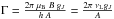$\mathrm{\Gamma }\mathrm{=}\frac{\mathrm{2}\mathit{\pi }{\mathit{\mu }}_{\mathrm{B}}\mathit{B}{\mathit{g}}_{\mathit{J}}}{\mathit{hA}}\mathrm{=}\frac{\mathrm{2}\mathit{\pi }{\mathit{\nu }}_{\mathrm{L}}{\mathit{g}}_{\mathit{J}}}{\mathit{A}}$. Note that ν_L is the Larmor frequency, h is the Planck constant, B is the magnetic field strength, μ_B is the Bohr magneton, g_J is the Landé factor of the J-level under consideration and A is the Einstein coefficient for the spontaneous emission of the spectral line having J as upper level. In particular, Γ = 1 corresponds to B = B_c, which is the critical magnetic field strength where the Hanle effect is maximal. For 0.1B_c<B< 10B_c, one may expect a sizable change of the scattering polarization signal with respect to the unmagnetized reference case. Numerically, one has 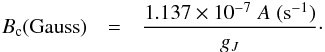$\begin{array}{ccc}{\mathit{B}}_{\mathrm{c}}\mathrm{\left(}\mathrm{Gauss}\mathrm{\right)}& \mathrm{=}& \frac{\mathrm{1.137}\mathrm{\times }{\mathrm{10}}^{-7}\mathit{A}\mathrm{\left(}{\mathrm{s}}^{-1}\mathrm{\right)}}{{\mathit{g}}_{\mathit{J}}}\mathrm{·}\end{array}$(1)According to L-S coupling, one finds that ${\mathit{g}}_{\mathit{J}}\mathrm{=}\frac{\mathrm{4}}{\mathrm{3}}$ for the level ${}^{\mathrm{2}}\mathrm{P}_{\mathrm{3}\mathit{/}\mathrm{2}}$ of the Sr ii ion. The Einstein coefficient is A = 1.26 × 10⁸ s^-1 (NIST database¹). Thus, for the linear scattering polarization of the Sr ii λ4078 line, B_c = 10.75 Gauss. Therefore, the scattering polarization of the Sr ii λ4078 line is of great practical interest here because the magnetic field in the chromospheric level is around tens of Gauss. Measurement and interpretation of the polarization of the Sr ii λ4078 line provides an interesting tool to determine magnetic field in the chromosphere of the Sun where the solar magnetism is not very well known.

In fact, the Hanle effect in the solar Sr ii λ4078 line has been studied by Bianda et al. (1998; see also Bianda 2003). They obtained a magnetic field strength in the range of 5 to 10 Gauss. They concluded that the Sr ii line yields on average values 30% lower than those obtained via diagnostics based on the Ca iλ4227 line and they remarked that this discrepancy cannot be regarded as very significant because of the uncertainties on the collisional rate determination. They argued that in the higher layers of the solar atmosphere, where Sr ii is formed near the solar limb, the collision rate is low. Equations (11)−(13) of Bianda et al. (1998) provide the magnetic field strength B and the Hanle rotation angle, according to the theory adopted by these authors. It seems that the obained magnetic field is underestimated because the effect of elastic collisions (represented by γ_c in the theory adopted by Bianda et al. 1998) is underestimated². It is possible that, if the collisions are fully taken into account in the framework of a realistic atomic model, the Sr ii line should give magnetic field values similar to these obtained via diagnostics based on the Ca iλ4227 line.

2. Summary of the theory of depolarizing collisions

Isotropic collisional interactions of the emitting Sr ii atoms with nearby hydrogen atoms tend to reestablish thermodynamical equilibrium inside Sr ii levels, i.e., to equalize populations of the Zeeman sublevels and to destroy their coherences, and thus partially destroy the atomic polarization. Consequently, a depolarization of the Sr ii line arises from these isotropic collisions.

Collisions of neutral hydrogen with heavy atoms like Sr ii and Sr i are not currently accessible to fully quantum chemistry treatments. To argue this statement, we cite an example concerning quantum calculations associated with the P-level of the Sr i atom. In fact, the depolarizing rate of P-level of the Sr i was calculated with quantum methods by Faurobert-Scholl et al. (1995) and later by Kerkeni (2002). Interestingly, Kerkeni (2002) obtained a value about a factor 2 smaller than Faurobert-Scholl et al. (1995). This disagreement was not expected since in both cases a quantum approach was used. We believe that one possible reason for this discrepancy is the significant complication of ab initio quantum calculations of the interaction potential between H i and heavy atoms like Sr i leading to large error bars in the quantum calculations. Thus, for heavy atoms or ions like Sr ii and Sr i, one needs semiclassical methods to determine the depolarizing collisional rates. However, quantum chemistry rates associated with ions having small size (e.g., Na i, Mg i, Ca ii, etc.) are accurate and important in validating approached semiclassical methods. We used the available quantum chemistry rates associated with Ca ii ions to validate the semiclassical method of Derouich et al. (2004). In fact, Ca ii is smaller in size as compared to Sr ii ions, and its quantum-chemistry study is accurate and unproblematic; for Ca ii and neutral hydrogen collisions, the quantum interaction potentials are extensively reviewed in the literature.

Collisional depolarization and polarization transfer rates associatedwith levels of Sr ii are obtained from the carefully tested semiclassical method of Derouich et al. (2004), which was developed for isotropic collisions between neutral hydrogen atoms and simple ions. In fact, the ionized alkaline earth metals Be ii, Mg ii, Ca ii, Sr ii, and Ba ii are simple ions because they have only one valence electron above a filled subshell³. Therefore, the determination of collisional rates using the approached method developed by Derouich et al. (2004) is possible with a percentage of error lower than 10% (see Sect. 6 of Derouich et al. 2004).

Derouich et al. (2004) applied their semi-classical method to obtain depolarization and polarization transfer rates for the upper level 5p²P of the Sr ii λ4078 line. The present work provides new depolarization and polarization transfer rates associated with the 4d ²D, which are indispensable for a rigorous analysis of the polarization of the Sr ii λ4078 line.

We describe the Sr ii atomic states by the density matrix elements ${\mathit{\rho }}_{\mathit{q}}^{\mathit{k}}\mathrm{\left(}\mathit{J}\mathrm{\right)}$ where 0 ≤ k ≤ 2J and −k ≤ q ≤ k. More details about the physical meaning of the tensorial order k and the coherence q could be found, for instance, in Omont (1977), Sahal-Bréchot (1977), and Landi Degl’Innocenti & Landolfi (2004).

According to Eq. (1) of Derouich et al. (2004), the variation of ${\mathit{\rho }}_{\mathit{q}}^{\mathit{k}}\mathrm{\left(}\mathit{J}\mathrm{\right)}$ due to isotropic collisions is: $\begin{array}{ccc}{\left[\frac{\mathrm{d}{\mathit{\rho }}_{\mathit{q}}^{\mathit{k}}\mathrm{(}\mathit{J}\mathrm{)}}{\mathrm{d}\mathit{t}}\right]}_{\mathrm{coll}}& \mathrm{=}& \mathrm{-}\left[\sum _{{\mathit{J}}^{\mathrm{\prime }}\ne \mathit{J}}\mathit{\zeta }\mathrm{(}\mathit{J}\mathrm{\to }{\mathit{J}}^{\mathrm{\prime }}\mathrm{)}\mathrm{+}{\mathit{D}}^{\mathit{k}}\mathrm{\left(}\mathit{J}\mathrm{\right)}\right]\mathrm{\times }{\mathit{\rho }}_{\mathit{q}}^{\mathit{k}}\mathrm{\left(}\mathit{J}\mathrm{\right)}\\ & & \mathrm{+}\sum _{{\mathit{J}}^{\mathrm{\prime }}\ne \mathit{J}}{\mathit{C}}^{\mathit{k}}\mathrm{(}{\mathit{J}}^{\mathrm{\prime }}\mathrm{\to }\mathit{J}\mathrm{)}\mathrm{\times }{\mathit{\rho }}_{\mathit{q}}^{\mathit{k}}\mathrm{\left(}{\mathit{J}}^{\mathrm{\prime }}\mathrm{\right)}\end{array}$(2)where C^k(J′ → J) are the polarization transfer rates, D^k(J) are the depolarization rates, and ζ(J → J′) are the fine structure transfer rates given by (Eq. (4) of Derouich et al. 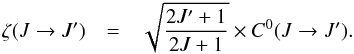2003b): $\begin{array}{ccc}\mathit{\zeta }\mathrm{(}\mathit{J}\mathrm{\to }{\mathit{J}}^{\mathrm{\prime }}\mathrm{)}& \mathrm{=}& \sqrt{\frac{\mathrm{2}{\mathit{J}}^{\mathrm{\prime }}\mathrm{+}\mathrm{1}}{\mathrm{2}\mathit{J}\mathrm{+}\mathrm{1}}}\mathrm{\times }{\mathit{C}}^{\mathrm{0}}\mathrm{(}\mathit{J}\mathrm{\to }{\mathit{J}}^{\mathrm{\prime }}\mathrm{)}\mathit{.}\end{array}$(3)Thus⁴, $\begin{array}{ccc}{\left[\frac{\mathrm{d}{\mathit{\rho }}_{\mathit{q}}^{\mathit{k}}\mathrm{(}\mathit{J}\mathrm{)}}{\mathrm{d}\mathit{t}}\right]}_{\mathrm{coll}}& \mathrm{=}& \mathrm{-}\left[\sum _{{\mathit{J}}^{\mathrm{\prime }}\ne \mathit{J}}\sqrt{\frac{\mathrm{2}{\mathit{J}}^{\mathrm{\prime }}\mathrm{+}\mathrm{1}}{\mathrm{2}\mathit{J}\mathrm{+}\mathrm{1}}}{\mathit{C}}^{\mathrm{0}}\mathrm{(}\mathit{J}\mathrm{\to }{\mathit{J}}^{\mathrm{\prime }}\mathrm{)}\mathrm{+}{\mathit{D}}^{\mathit{k}}\mathrm{\left(}\mathit{J}\mathrm{\right)}\right]\mathrm{\times }{\mathit{\rho }}_{\mathit{q}}^{\mathit{k}}\mathrm{\left(}\mathit{J}\mathrm{\right)}\\ & & \mathrm{+}\hspace{0.17em}\sum _{{\mathit{J}}^{\mathrm{\prime }}\ne \mathit{J}}{\mathit{C}}^{\mathit{k}}\mathrm{(}{\mathit{J}}^{\mathrm{\prime }}\mathrm{\to }\mathit{J}\mathrm{)}\mathrm{\times }{\mathit{\rho }}_{\mathit{q}}^{\mathit{k}}\mathrm{\left(}{\mathit{J}}^{\mathrm{\prime }}\mathrm{\right)}\mathit{.}\end{array}$(4)Now we denote the collisional transfer rates C^k(J′ → J) by ${\mathit{C}}_{\mathrm{I}}^{\mathrm{\left(}\mathit{k}\mathrm{\right)}}\mathrm{(}{\mathit{J}}^{\mathrm{\prime }}\mathrm{\to }\mathit{J}\mathrm{)}$ if J′ = J_l<J (inelastic collisions) and we notice C^k(J′ → J) by ${\mathit{C}}_{\mathrm{S}}^{\mathrm{\left(}\mathit{k}\mathrm{\right)}}\mathrm{(}{\mathit{J}}^{\mathrm{\prime }}\mathrm{\to }\mathit{J}\mathrm{)}$ if J′ = J_u>J (super-elastic collisions). We find: $\begin{array}{ccc}{\left[\frac{\mathrm{d}{\mathit{\rho }}_{\mathit{q}}^{\mathit{k}}\mathrm{(}\mathit{J}\mathrm{)}}{\mathrm{d}\mathit{t}}\right]}_{\mathrm{coll}}& \mathrm{=}& \mathrm{-}[\sum _{{\mathit{J}}_{\mathit{l}}\ne \mathit{J}}\sqrt{\frac{\mathrm{2}{\mathit{J}}_{\mathit{l}}\mathrm{+}\mathrm{1}}{\mathrm{2}\mathit{J}\mathrm{+}\mathrm{1}}}{\mathit{C}}_{\mathrm{S}}^{\mathrm{0}}\mathrm{(}\mathit{J}\mathrm{\to }{\mathit{J}}_{\mathit{l}}\mathrm{)}\\ & & \mathrm{+}\sum _{{\mathit{J}}_{\mathit{u}}\ne \mathit{J}}\sqrt{\frac{\mathrm{2}{\mathit{J}}_{\mathit{u}}\mathrm{+}\mathrm{1}}{\mathrm{2}\mathit{J}\mathrm{+}\mathrm{1}}}{\mathit{C}}_{\mathrm{I}}^{\mathrm{0}}\mathrm{(}\mathit{J}\mathrm{\to }{\mathit{J}}_{\mathit{u}}\mathrm{)}\mathrm{+}{\mathit{D}}^{\mathit{k}}\mathrm{\left(}\mathit{J}\mathrm{\right)}]\mathrm{\times }{\mathit{\rho }}_{\mathit{q}}^{\mathit{k}}\mathrm{\left(}\mathit{J}\mathrm{\right)}\\ & & \mathrm{+}\sum _{{\mathit{J}}_{\mathit{l}}\ne \mathit{J}}{\mathit{C}}_{\mathrm{I}}^{\mathit{k}}\mathrm{(}{\mathit{J}}_{\mathit{l}}\mathrm{\to }\mathit{J}\mathrm{)}\mathrm{\times }{\mathit{\rho }}_{\mathit{q}}^{\mathit{k}}\mathrm{\left(}{\mathit{J}}_{\mathit{l}}\mathrm{\right)}\mathrm{+}\sum _{{\mathit{J}}_{\mathit{u}}\ne \mathit{J}}{\mathit{C}}_{\mathrm{S}}^{\mathit{k}}\mathrm{(}{\mathit{J}}_{\mathit{u}}\mathrm{\to }\mathit{J}\mathrm{)}\mathrm{\times }{\mathit{\rho }}_{\mathit{q}}^{\mathit{k}}\mathrm{\left(}{\mathit{J}}_{\mathit{u}}\mathrm{\right)}\mathit{.}\end{array}$(5)We denote by R^k(J) the relaxation rates of rank k given by (Eq. (2) of Derouich 2008): $\begin{array}{ccc}{\mathit{R}}^{\mathit{k}}\mathrm{\left(}\mathit{J}\mathrm{\right)}& \mathrm{=}& \sum _{{\mathit{J}}_{\mathit{l}}\ne \mathit{J}}\sqrt{\frac{\mathrm{2}{\mathit{J}}_{\mathit{l}}\mathrm{+}\mathrm{1}}{\mathrm{2}\mathit{J}\mathrm{+}\mathrm{1}}}{\mathit{C}}_{\mathrm{S}}^{\mathrm{0}}\mathrm{(}\mathit{J}\mathrm{\to }{\mathit{J}}_{\mathit{l}}\mathrm{)}\\ & & \mathrm{+}\sum _{{\mathit{J}}_{\mathit{u}}\ne \mathit{J}}\sqrt{\frac{\mathrm{2}{\mathit{J}}_{\mathit{u}}\mathrm{+}\mathrm{1}}{\mathrm{2}\mathit{J}\mathrm{+}\mathrm{1}}}{\mathit{C}}_{\mathrm{I}}^{\mathrm{0}}\mathrm{(}\mathit{J}\mathrm{\to }{\mathit{J}}_{\mathit{u}}\mathrm{)}\mathrm{+}{\mathit{D}}^{\mathit{k}}\mathrm{\left(}\mathit{J}\mathrm{\right)}\mathit{.}\end{array}$(6)Then, $\begin{array}{ccc}{\left[\frac{\mathrm{d}{\mathit{\rho }}_{\mathit{q}}^{\mathit{k}}\mathrm{(}\mathit{J}\mathrm{)}}{\mathrm{d}\mathit{t}}\right]}_{\mathrm{coll}}& \mathrm{=}& \mathrm{-}{\mathit{R}}^{\mathit{k}}\mathrm{\left(}\mathit{J}\mathrm{\right)}\mathrm{\times }{\mathit{\rho }}_{\mathit{q}}^{\mathit{k}}\mathrm{\left(}\mathit{J}\mathrm{\right)}\mathrm{+}\sum _{{\mathit{J}}_{\mathit{l}}\ne \mathit{J}}{\mathit{C}}_{\mathrm{I}}^{\mathit{k}}\mathrm{(}{\mathit{J}}_{\mathit{l}}\mathrm{\to }\mathit{J}\mathrm{)}\mathrm{\times }{\mathit{\rho }}_{\mathit{q}}^{\mathit{k}}\mathrm{\left(}{\mathit{J}}_{\mathit{l}}\mathrm{\right)}\\ & & \mathrm{+}\sum _{{\mathit{J}}_{\mathit{u}}\ne \mathit{J}}{\mathit{C}}_{\mathrm{S}}^{\mathit{k}}\mathrm{(}{\mathit{J}}_{\mathit{u}}\mathrm{\to }\mathit{J}\mathrm{)}\mathrm{\times }{\mathit{\rho }}_{\mathit{q}}^{\mathit{k}}\mathrm{\left(}{\mathit{J}}_{\mathit{u}}\mathrm{\right)}\mathit{,}\end{array}$(7)which is the same as the Eq. (3) given in Derouich (2008). Physically, the collisional relaxation rates R^k(J) correspond to the loss of atomic polarization and, in contrast, the transfer rates ${\mathit{C}}_{\mathrm{I}}^{\mathit{k}}\mathrm{(}{\mathit{J}}_{\mathit{l}}\mathrm{\to }\mathit{J}\mathrm{)}$ and ${\mathit{C}}_{\mathrm{S}}^{\mathit{k}}\mathrm{(}{\mathit{J}}_{\mathit{u}}\mathrm{\to }\mathit{J}\mathrm{)}$ correspond to the gain of atomic polarization coming from other levels.

In the literature, there are different definitions of the collisional rates, and these definitions must be taken into account when writing the Eq. (9) to calculate polarization signals correctly. For this reason, Eqs. (4)−(9) are necessary for a reader who wants to exploit our paper. For example, the depolarization rates as defined in our work, as compared to those defined by Kerkeni et al. (2003), are not equivalent. Derouich et al. (2004, Sect. 7) confronted this problem when they wanted to compare their rates with the collisional rates obtained by Kerkeni et al. (2003). In adiition, there is a small difference between the definition of our collisional rates and the definition of the collisional rates obtained in Landi Degl’Innocenti & Landolfi (2004).

Note that the observed linear polarization of the Sr iiλ4078 line is the footprint of only the even orders k inside the Sr ii atom, and thus only depolarization and polarization transfer rates with even k are needed to study this line. In addition, since the collisions are isotropic, all collisional rates are q-independent.

3. Calculation of the collisional rates for the modeling of the Sr II λ4078 Å line

Generally speaking, studying the polarization of the Sr iiλ4078 line implies that we are solving the radiative transfer equations for polarized radiation in a magnetized atmosphere. To be able to solve these equations numerically, one should adopt a simplified atomic model, such as the one presented in Fig. 1. Particularly, in the framework of the simplified model, one disregards the effects of the metastable D-states in the Sr iiλ4078 line modeling (see Bianda et al. 1998).

Our intention is to complete these models by taking the effect of collisions on the D-states into account. To this aim, we consider a realistic multilevels and multilines atomic model of Fig. 2 (hereafter the full model). It contains the five levels: S_1/2, P_1/2, P_3/2, D_3/2 and D_5/2 and five lines: λ = 10 915Å, λ = 10 327Å, λ = 10 036Å, λ = 4216Å, and λ = 4078Å.

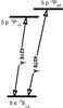Fig. 1 Partial Grotrian diagram of Sr ii showing the levels and the spectral wavelengths taken into account in the case of the simplified model. Note that the level spacings are not to scale.

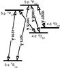Fig. 2 Partial Grotrian diagram of Sr ii showing the levels and the allowed radiative transitions used in the full model, which takes into account the metastable D-states. Note that the level spacings are not to scale.

We apply our collisional numerical code to calculate the collisional scattering matrix after integration of the semiclassical differential coupled equations, which are derived from the time dependent Schrödinger equation. Once the scattering matrix is obtained for the P- and D-states of Sr ii, we determine the transition probabilities in the tensorial irreducible basis. Afterward, these propabilities are integrated over impact parameters and Maxwellian distribution of relative velocities to obtain depolarization and transfer rates. We perform calculations by varying the temperature to obtain the best analytical fit to the collisional rates. The precision on the Sr ii rates should be similar to the precision obtained on the Ca ii rates (Derouich et al. 2004), i.e., better than 10%.

Derouich et al. 2004 derived the following expressions of needed depolarization and polarization transfer rates by isotropic collisions of P-levels of Sr ii ions with neutral hydrogen⁵: 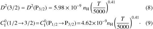$\begin{array}{ccc}& & {\mathit{D}}^{\mathrm{2}}\mathrm{(}\mathrm{3}\mathit{/}\mathrm{2}\mathrm{)}\mathrm{=}{\mathit{D}}^{\mathrm{2}}\mathrm{\left(}{\mathrm{P}}_{\mathrm{3}\mathit{/}\mathrm{2}}\mathrm{\right)}\mathrm{=}\mathrm{5.98}\mathrm{\times }{\mathrm{10}}^{-9}{\mathit{n}}_{\mathrm{H}}{\left(\frac{\mathit{T}}{\mathrm{5000}}\right)}^{\mathrm{0.41}} \\ & & {\mathit{C}}_{\mathrm{I}}^{\mathrm{0}}\mathrm{(}\mathrm{1}\mathit{/}\mathrm{2}\mathrm{\to }\mathrm{3}\mathit{/}\mathrm{2}\mathrm{)}\mathrm{=}{\mathit{C}}_{\mathrm{I}}^{\mathrm{0}}\mathrm{(}{\mathrm{P}}_{\mathrm{1}\mathit{/}\mathrm{2}}\mathrm{\to }{\mathrm{P}}_{\mathrm{3}\mathit{/}\mathrm{2}}\mathrm{)}\mathrm{=}\mathrm{4.62}\mathrm{\times }{\mathrm{10}}^{-9}{\mathit{n}}_{\mathrm{H}}{\left(\frac{\mathit{T}}{\mathrm{5000}}\right)}^{\mathrm{0.41}}\mathrm{·} \end{array}$In addition, in the present work, we provide the following new expressions of collisional rates associated with the D-levels: 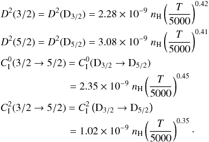$\begin{array}{ccc}& & {\mathit{D}}^{\mathrm{2}}\mathrm{(}\mathrm{3}\mathit{/}\mathrm{2}\mathrm{)}\mathrm{=}{\mathit{D}}^{\mathrm{2}}\mathrm{\left(}{\mathrm{D}}_{\mathrm{3}\mathit{/}\mathrm{2}}\mathrm{\right)}\mathrm{=}\mathrm{2.28}\mathrm{\times }{\mathrm{10}}^{-9}{\mathit{n}}_{\mathrm{H}}{\left(\frac{\mathit{T}}{\mathrm{5000}}\right)}^{\mathrm{0.42}}\\ & & {\mathit{D}}^{\mathrm{2}}\mathrm{(}\mathrm{5}\mathit{/}\mathrm{2}\mathrm{)}\mathrm{=}{\mathit{D}}^{\mathrm{2}}\mathrm{\left(}{\mathrm{D}}_{\mathrm{5}\mathit{/}\mathrm{2}}\mathrm{\right)}\mathrm{=}\mathrm{3.08}\mathrm{\times }{\mathrm{10}}^{-9}{\mathit{n}}_{\mathrm{H}}{\left(\frac{\mathit{T}}{\mathrm{5000}}\right)}^{\mathrm{0.41}}\\ & & {\mathit{C}}_{\mathrm{I}}^{\mathrm{0}}\mathrm{(}\mathrm{3}\mathit{/}\mathrm{2}\mathrm{\to }\mathrm{5}\mathit{/}\mathrm{2}\mathrm{)}\mathrm{=}{\mathit{C}}_{\mathrm{I}}^{\mathrm{0}}\mathrm{(}{\mathrm{D}}_{\mathrm{3}\mathit{/}\mathrm{2}}\mathrm{\to }{\mathrm{D}}_{\mathrm{5}\mathit{/}\mathrm{2}}\mathrm{)}\\ & & \mathrm{=}\mathrm{2.35}\mathrm{\times }{\mathrm{10}}^{-9}{\mathit{n}}_{\mathrm{H}}{\left(\frac{\mathit{T}}{\mathrm{5000}}\right)}^{\mathrm{0.45}}\\ & & {\mathit{C}}_{\mathrm{I}}^{\mathrm{2}}\mathrm{(}\mathrm{3}\mathit{/}\mathrm{2}\mathrm{\to }\mathrm{5}\mathit{/}\mathrm{2}\mathrm{)}\mathrm{=}{\mathit{C}}_{\mathrm{I}}^{\mathrm{2}}\left({\mathrm{D}}_{\mathrm{3}\mathit{/}\mathrm{2}}\mathrm{\to }{\mathrm{D}}_{\mathrm{5}\mathit{/}\mathrm{2}}\right)\\ & & \mathrm{=}\mathrm{1.02}\mathrm{\times }{\mathrm{10}}^{-9}{\mathit{n}}_{\mathrm{H}}{\left(\frac{\mathit{T}}{\mathrm{5000}}\right)}^{\mathrm{0.35}}\mathrm{·}\end{array}$(10)All rates are given in s^-1. Only the depolarization rates D^{k = 2}(J) and inelastic collisional rates ${\mathit{C}}_{\mathrm{I}}^{\mathit{k}}\mathrm{(}{\mathit{J}}_{\mathit{l}}\mathrm{\to }\mathit{J}\mathrm{)}$ with k = 0 and 2 are given as a function of neutral hydrogen number density n_H (in cm^-3) and kinetic temperature T (in K). Note that, given the low degree of radiation anisotropy in the solar atmosphere, one can safely neglect the effect of D⁴(5/2) on the linear polarization of the Sr ii λ4078 line. However, one can retrieve the values of the superelastic collisional rates ${\mathit{C}}_{\mathrm{S}}^{\mathit{k}}\mathrm{(}{\mathit{J}}_{\mathit{u}}\mathrm{\to }\mathit{J}\mathrm{)}$ by applying the detailed balance relationship: 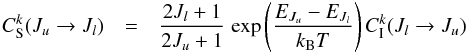$\begin{array}{ccc}{\mathit{C}}_{\mathrm{S}}^{\mathit{k}}\mathrm{(}{\mathit{J}}_{\mathit{u}}\mathrm{\to }{\mathit{J}}_{\mathit{l}}\mathrm{)}& \mathrm{=}& \frac{\mathrm{2}{\mathit{J}}_{\mathit{l}}\mathrm{+}\mathrm{1}}{\mathrm{2}{\mathit{J}}_{\mathit{u}}\mathrm{+}\mathrm{1}}\exp \left(\frac{{\mathit{E}}_{{\mathit{J}}_{\mathit{u}}}\mathrm{-}{\mathit{E}}_{{\mathit{J}}_{\mathit{l}}}}{{\mathit{k}}_{\mathrm{B}}\mathit{T}}\right){\mathit{C}}_{\mathrm{I}}^{\mathit{k}}\mathrm{(}{\mathit{J}}_{\mathit{l}}\mathrm{\to }{\mathit{J}}_{\mathit{u}}\mathrm{)}\end{array}$(11)with E_Ju and E_Jl being the energy of the upper level J_u and the lower level J_l, respectively. Note that k_B is the Boltzmann constant.

It is important to notice that the Eq. (11) is valid only in the case of the Maxwell distribution of the velocities of the hydrogen atoms, but the dimensionless collision strength (generally denoted by Ω) must be symmetrical also, i.e., Ω(J_u → J_l) = Ω(J_l → J_u). The term “collision strength” was originally suggested by Seaton (1953, 1955) and is now universally used. The collision strength Ω contains the information about the collisional transition probability between two given levels and it is ultimately related to the scattering matrix. In our collisional method, the interaction potential matrix is hermitian, which implies that the scattering S-matrix is unitary and symmetric (Derouich et al. 2003a). Consequently, Ω is symmetrical and the Eq. (11) is well satisfied.

By taking E_Ju and E_Jl from NIST database, one finds at T = 6000 K: 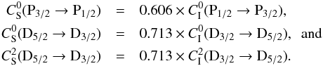$\begin{array}{ccc}{\mathit{C}}_{\mathrm{S}}^{\mathrm{0}}\mathrm{(}{\mathrm{P}}_{\mathrm{3}\mathit{/}\mathrm{2}}\mathrm{\to }{\mathrm{P}}_{\mathrm{1}\mathit{/}\mathrm{2}}\mathrm{)}& \mathrm{=}& \mathrm{0.606}\mathrm{\times }{\mathit{C}}_{\mathrm{I}}^{\mathrm{0}}\mathrm{(}{\mathrm{P}}_{\mathrm{1}\mathit{/}\mathrm{2}}\mathrm{\to }{\mathrm{P}}_{\mathrm{3}\mathit{/}\mathrm{2}}\mathrm{)}\mathit{,}\\ {\mathit{C}}_{\mathrm{S}}^{\mathrm{0}}\mathrm{(}{\mathrm{D}}_{\mathrm{5}\mathit{/}\mathrm{2}}\mathrm{\to }{\mathrm{D}}_{\mathrm{3}\mathit{/}\mathrm{2}}\mathrm{)}& \mathrm{=}& \mathrm{0.713}\mathrm{\times }{\mathit{C}}_{\mathrm{I}}^{\mathrm{0}}\mathrm{(}{\mathrm{D}}_{\mathrm{3}\mathit{/}\mathrm{2}}\mathrm{\to }{\mathrm{D}}_{\mathrm{5}\mathit{/}\mathrm{2}}\mathrm{)}\mathit{,}\mathrm{and}\\ {\mathit{C}}_{\mathrm{S}}^{\mathrm{2}}\mathrm{(}{\mathrm{D}}_{\mathrm{5}\mathit{/}\mathrm{2}}\mathrm{\to }{\mathrm{D}}_{\mathrm{3}\mathit{/}\mathrm{2}}\mathrm{)}& \mathrm{=}& \mathrm{0.713}\mathrm{\times }{\mathit{C}}_{\mathrm{I}}^{\mathrm{2}}\mathrm{(}{\mathrm{D}}_{\mathrm{3}\mathit{/}\mathrm{2}}\mathrm{\to }{\mathrm{D}}_{\mathrm{5}\mathit{/}\mathrm{2}}\mathrm{)}\mathit{.}\end{array}$(12)

4. Scattering polarization of the Sr II λ4078 line

In theory, the core of the Sr ii λ4078 line is formed at the chromosphere but the wings are formed in deeper layers of the photosphere. Since the density of hydrogen atoms n_H in the photosphere is larger than n_H in the chromosphere, if the effect of collisions cannot be neglected for the core of the Sr ii λ4078, then collisions cannot be neglected in the wings of that line.

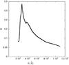Fig. 3 Anisotropy factor $\mathit{w}\mathrm{\left(}\mathit{\lambda }\mathrm{\right)}\mathrm{=}\sqrt{\mathrm{2}}\mathrm{(}{\mathit{J}}_{\mathrm{0}}^{\mathrm{2}}\mathit{/}{\mathit{J}}_{\mathrm{0}}^{\mathrm{0}}\mathrm{)}$ given as a function of the wavelengths.

We consider that the solar chromosphere is a plane-parallel layer formed by Sr ii ions, which are excited anisotropically from below by the photospheric radiation. The components of the incident radiation field at the wavelength λ = 4078 Å are usually denoted by ${\mathit{J}}_{\mathit{q}}^{\mathit{k}}$ where k is the tensorial order and q represents the coherences in the tensorial basis (−k ≤ q ≤ k); the order k can be equal to 0 (with q = 0) or 2 (with q = 0, ±1, ±2). This radiation field with six components constitutes a generalization of the unpolarized light field where only the quantity ${\mathit{J}}_{\mathrm{0}}^{\mathrm{0}}$ is considered. In fact, ${\mathit{J}}_{\mathrm{0}}^{\mathrm{0}}$ is proportional to the intensity of the radiation. If the chromosphere is assumed to be uniform, the radiation has a cylindrical symmetry around its preferred direction implying that the coherence components with q ≠ 0 are zero. In fact, ${\mathit{J}}_{\mathit{q}\mathrm{=}\mathrm{\pm }\mathrm{1}}^{\mathit{k}\mathrm{=}\mathrm{2}}$ and ${\mathit{J}}_{\mathit{q}\mathrm{=}\mathrm{\pm }\mathrm{2}}^{\mathit{k}\mathrm{=}\mathrm{2}}$ components quantify the breaking of the cylindrical symmetry around the axis of quantification.

If the incident radiation is no longer anisotropic, the components ${\mathit{J}}_{\mathit{q}}^{\mathit{k}\mathrm{=}\mathrm{2}}$ become zero, which means that no linear polarization can be created as a result of scattering processes. Regardless of the anisotropy of the incident radiation, the radiation component associated with the circular polarization usually denoted by ${\mathit{J}}_{\mathit{q}}^{\mathit{k}\mathrm{=}\mathrm{1}}$ is negligible. This means that no odd order k can be created inside the scattering strontium ion. As a result, the Stokes V of the scattered radiation at λ = 4078 Å is zero.

We concentrate our study on the core of the Sr iiλ4078 line. Neglecting the possible presence of inhomogeneities of the chromospheric regions, the radiation field is cylindrically symmetrical around the vertical direction, and its properties are fully described by the two components ${\mathit{J}}_{\mathrm{0}}^{\mathrm{0}}\mathrm{(}\mathit{\lambda }\mathrm{=}\mathrm{4078}\AA \mathrm{)}$ and ${\mathit{J}}_{\mathrm{0}}^{\mathrm{2}}\mathrm{(}\mathit{\lambda }\mathrm{=}\mathrm{4078}\AA \mathrm{)}$ of the radiation field tensor or, alternatively, by the value of the anisotropy factor 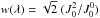$\mathit{w}\mathrm{\left(}\mathit{\lambda }\mathrm{\right)}\mathrm{=}\sqrt{\mathrm{2}}\mathrm{(}{\mathit{J}}_{\mathrm{0}}^{\mathrm{2}}\mathit{/}{\mathit{J}}_{\mathrm{0}}^{\mathrm{0}}\mathrm{)}$ and of the number of photons per mode 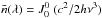$\mathit{n̅}\mathrm{\left(}\mathit{\lambda }\mathrm{\right)}\mathrm{=}{\mathit{J}}_{\mathrm{0}}^{\mathrm{0}}\mathrm{(}{\mathit{c}}^{\mathrm{2}}\mathit{/}\mathrm{2}\mathit{h}{\mathit{\nu }}^{\mathrm{3}}\mathrm{)}$ (see, e.g., Trujillo Bueno 2001; Manso Sainz & Landi Degl’Innocenti 2002). We notice that w(λ = 4078) and are obtained from Figs. 3 and 4; these figures were derived by Manso Sainz & Landi Degl’Innocenti (2002) from the center-to-limb variations of the continuum intensities in the quiet Sun provided by Cox (2000).

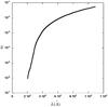Fig. 4 Number of photons per mode $\mathit{n̅}\mathrm{\left(}\mathit{\lambda }\mathrm{\right)}\mathrm{=}{\mathit{J}}_{\mathrm{0}}^{\mathrm{0}}\mathrm{(}{\mathit{c}}^{\mathrm{2}}\mathit{/}\mathrm{2}\mathit{h}{\mathit{\nu }}^{\mathrm{3}}\mathrm{)}$ given as a function of the wavelengths.

5. The correction factor f_c

Since we do not solve the radiative transfer equations for the Stokes parameters, our work should be considered as complementary to other investigations that focus on radiative transfer effects but neglect multilevel and collisional effects. Our aim is to provide a correction factor on the theoretical value of the line linear polarization obtained by solving the non-LTE radiative transfer problem in the framework of two-level modeling. In this sense, we recall that Faurobert et al. (2009) used a correction factor determined by Derouich (2008) for the Ba iiλ4554 line; they found that, using a correction factor, the accuracy on the magnetic field has been improved by ~50%.

The crorrection factor f_c must contain information on the difference between the value of [p] _simplified and [p] _full. Thus, it could be written as: $\begin{array}{ccc}{\mathit{f}}_{\mathrm{c}}& \mathrm{=}& \mathrm{(}\mathrm{[}\mathit{p}{\mathrm{]}}_{\mathrm{simplified}}\mathrm{-}\mathrm{[}\mathit{p}{\mathrm{]}}_{\mathrm{full}}\mathrm{)}\mathrm{\times }\mathrm{100.}\end{array}$(13)Note that [p] _simplified is the linear polarization inferred from considering the simplified model and [p] _full is the linear polarization inferred from considering the full model. Obviously, [p] _simplified and [p] _full are calculated in the presence of collisions which means that f_c is a function of n_H.

We consider that the evolution of the density-matrix elements is due to the collisional and radiative effects. To calculate the linear polarization degree p = Q/I, we use the formulae of Trujillo Bueno (1999): $\begin{array}{ccc}\mathit{Q}\mathit{/}\mathit{I}& & \mathrm{=}\frac{\mathrm{3}}{\mathrm{2}\sqrt{\mathrm{2}}}\mathrm{[}{\mathit{\omega }}_{{\mathit{J}}_{\mathit{u}}{\mathit{J}}_{\mathit{l}}}^{\mathrm{\left(}\mathrm{2}\mathrm{\right)}}{\mathit{\sigma }}_{\mathrm{0}}^{\mathrm{2}}\mathrm{\left(}\mathit{u}\mathrm{\right)}\mathrm{-}{\mathit{\omega }}_{{\mathit{J}}_{\mathit{l}}{\mathit{J}}_{\mathit{u}}}^{\mathrm{\left(}\mathrm{2}\mathrm{\right)}}{\mathit{\sigma }}_{\mathrm{0}}^{\mathrm{2}}\mathrm{(}\mathit{l}{\mathrm{)}}^{\mathrm{]}}\mathit{,}\end{array}$(14)which gives the linear polarization degree at the limit of tangential observation, i.e., at zero altitude above the solar limb. The indices l (for lower) and u (for upper) denote lower level J_l and upper J_u of the transition. ${\mathit{\omega }}_{\mathit{J}{\mathit{J}}^{\mathrm{\prime }}}^{\mathrm{\left(}\mathit{k}\mathrm{\right)}}$ is a numerical coefficient introduced and tabulated for various values of k, J, and J′ in Landi Degl’Innocenti (1984). ${\mathit{\sigma }}_{\mathrm{0}}^{\mathit{k}}\mathrm{=}{\mathit{\rho }}_{\mathrm{0}}^{\mathit{k}}\mathit{/}{\mathit{\rho }}_{\mathrm{0}}^{\mathrm{0}}$, where ${\mathit{\rho }}_{\mathrm{0}}^{\mathit{k}}$ are the solutions of the statistical equilibrium equations (SEE) including collisional and radiative rates: $\begin{array}{ccc}\left[\frac{\mathrm{d}{\mathit{\rho }}_{\mathrm{0}}^{\mathit{k}}\mathrm{\left(}\mathit{J}\mathrm{\right)}}{\mathrm{d}\mathit{t}}\right]& \mathrm{=}& {\left[\frac{\mathrm{d}{\mathit{\rho }}_{\mathrm{0}}^{\mathit{k}}\mathrm{\left(}\mathit{J}\mathrm{\right)}}{\mathrm{d}\mathit{t}}\right]}_{\mathrm{coll}}\mathrm{+}{\left[\frac{\mathrm{d}{\mathit{\rho }}_{\mathrm{0}}^{\mathit{k}}\mathrm{\left(}\mathit{J}\mathrm{\right)}}{\mathrm{d}\mathit{t}}\right]}_{\mathrm{rad}}\mathrm{=}\mathrm{0.}\end{array}$(15)For atmospheric levels where the hydrogen density n_H ~ 10¹⁵ cm^-3 and T ~ 6000 K, D²(P_3/2) ~ 6.4 × 10⁶ s^-1 ≪ A = 1.26 × 10⁸s^-1. Because the inverse lifetime of the upper level of the Sr ii λ4078 line is greater than the value of the elastic depolarizing rate D²(P_3/2), one might think that the effect of the collisions is negligible. We will demonstrate that at n_H ~ 10¹⁵ the effect of collisions cannot be neglected.

We solve the SEE to calculate the ${\mathit{\rho }}_{\mathrm{0}}^{\mathit{k}}$ elements and thus we determine the linear polarization p = Q/I of the Sr ii λ4078 line once by using the simplified atomic model (see Fig. 1) and once by using the full model (see Fig. 2) that accounts for the metastable D-levels. We then investigate the sensitivity of the emergent linear polarization to the above-mentioned collisions to point out the range of n_H where the effect of collisions is important. Since the collisional rates are proportional to the hydrogen density (the impact approximation), determining the dependence of the polarization to collisional rates amounts to the study of its dependence on n_H.

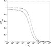Fig. 5 Linear polarization ratio [p] simplified/ [p] max as a function of nH plotted as ..°..-symbols. [p] full/ [p] max as a function of nH plotted as −⋄−-symbols.

Figure 5 represents the linear polarization inferred from the simplified model in the presence of collisions, [p] _simplified, divided by [p] _max, which is the zero-collisions polarization inferred from the simplified model. In addition, Fig. 5 shows the ratio [p] _full/ [p] _max giving the linear polarization inferred from the full model in the presence of collisions divided by the same [p] _max.

Looking to Fig. 5, the upper horizontal line with ..°..-symbols represents the polarization scattered without any sensitive collision effects. In fact, according to Fig. 5, for n_H< 7 × 10¹⁴ cm^-3 the variation of [p] _simplified is smaller that 2%, i.e., the ratio [p] _simplified/ [p] _max ≃ 1 > 0.98. For n_H> 7 × 10¹⁴ cm^-3, the ratio [p] _simplified/ [p] _max starts to decrease progressively which reflects the collisional destruction of the alignment of the ²P_3/2 level. At n_H> 3 × 10¹⁷ cm^-3, [p] _simplified/ [p] _max< 0.1, thus the linear atomic polarization in the level ${}^{\mathrm{2}}\mathit{P}_{\mathrm{3}\mathit{/}\mathrm{2}}$ is almost completely destroyed and [p] _simplified ≃ 0.

Referring again to Fig. 5, the upper horizontal line with −⋄−-symbols corresponds to the scattering polarization obtained using the full model in a range of n_H where collisions are negligible, i.e., for n_H< 1 × 10¹⁴ cm^-3 where [p] _full/ [p] _max ≃ constant > 0.93. It is important to notice that [p] _full/ [p] _max ≠ 1 even in the range where collisions are negligible, which is beacause the simplified model overestimates the polarization degree usually leading to the fact that [p] _full/ [p] _max< 1. For n_H> 3 × 10¹⁴ cm^-3, the ratio [p] _full/ [p] _max starts to decrease progressively which reflects the collisional destruction of the alignment of the ²D_3/2 and ²D_5/2 levels. At n_H ≃ 3 × 10¹⁴ cm^-3, the alignment of the level ²P_3/2 is not affected yet by collisions but the polarization of Sr ii λ4078 line decreases via the destruction of the alignment of the D-levels. For n_H = 4 × 10¹⁵ cm^-3, the [p] _full/ [p] _max = 0.74, meaning that collisions and multilevels effects result in a decrease of the polarization degree by more than 25%; note that at the same n_H = 4 × 10¹⁵ cm^-3 one has [p] _simplified/ [p] _max = 0.9.

In order to take into account the effect of elastic collisions and of alignment transfer due to multilevel coupling with the metastable D-levels, one must determine the correction factor f_c = ( [p] _simplified − [p] _full) × 100 for each n_H. For instance at n_H = 4 × 10¹⁵ cm^-3, f_c = (0.9−0.74) × 100 = 16%. Figure 6 shows the variation of f_c as a function of n_H. For ≃4 × 10¹⁴<n_H< 5 × 10¹⁷, the determination of f_c is crucial for a correct determination of linear polarization.

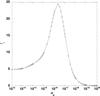Fig. 6 Correction factor fc as a function of nH. fc must be applied to the value of the linear polarization derived from the simplified model.

6. Conclusion

We use our collisional approach and our numerical code to calculate new collisional rates associated with the D-states of Sr ii, and using another numerical code, we calculate the polarization of the Sr ii line by including our collisional rates in the statistical equilibrium of a Sr ii model atom. Our aim was to pay particular attention to a subtle collisional depolarizing effect of the Sr ii λ4078 line due to the metastable D-levels. This should help to provide key elements to analyze quantitatively the scattering polarization of the Sr ii λ4078 line. In fact, we find that the Sr iiλ4078 line could be collisionally depolarized even when its upper level ²P_3/2 is not affected by collisions. A given model can correctly reproduce the observed scattering polarization only if one takes properly into account the collisional perturbation of the atmoic levels by the interaction with nearby hydrogen atoms. It is important to notice that our results have to be considered as information complementary to the models taking radiative transfer into account but without taking properly into account the effect of collisions in realistic multilevel schemes.

As the scattering polarization degree is usually rather small (e.g., polarization of the order of 1% in Fraunhofer lines in the photosphere and chromosphere of the Sun), careful and rigorous modeling of that polarization is of fundamental importance for learning especially about a weak and even unresolved magnetic field by its Hanle effect.

References

All Tables

All Figures

	Fig. 1 Partial Grotrian diagram of Sr ii showing the levels and the spectral wavelengths taken into account in the case of the simplified model. Note that the level spacings are not to scale.
In the text

	Fig. 2 Partial Grotrian diagram of Sr ii showing the levels and the allowed radiative transitions used in the full model, which takes into account the metastable D-states. Note that the level spacings are not to scale.
In the text

	Fig. 3 Anisotropy factor $\mathit{w}\mathrm{\left(}\mathit{\lambda }\mathrm{\right)}\mathrm{=}\sqrt{\mathrm{2}}\mathrm{(}{\mathit{J}}_{\mathrm{0}}^{\mathrm{2}}\mathit{/}{\mathit{J}}_{\mathrm{0}}^{\mathrm{0}}\mathrm{)}$ given as a function of the wavelengths.
In the text

	Fig. 4 Number of photons per mode $\mathit{n̅}\mathrm{\left(}\mathit{\lambda }\mathrm{\right)}\mathrm{=}{\mathit{J}}_{\mathrm{0}}^{\mathrm{0}}\mathrm{(}{\mathit{c}}^{\mathrm{2}}\mathit{/}\mathrm{2}\mathit{h}{\mathit{\nu }}^{\mathrm{3}}\mathrm{)}$ given as a function of the wavelengths.
In the text

	Fig. 5 Linear polarization ratio [p] simplified/ [p] max as a function of nH plotted as ..°..-symbols. [p] full/ [p] max as a function of nH plotted as −⋄−-symbols.
In the text

	Fig. 6 Correction factor fc as a function of nH. fc must be applied to the value of the linear polarization derived from the simplified model.
In the text

References

- Berdyugina, S. V., & Fluri, D. M. 2004, 417, 775 [Google Scholar]
- Bianda, M. 2003, Ph.D. Thesis, ETH Zr¨ich (Göttingen: Cuvillier) [Google Scholar]
- Bianda, M., & Stenflo, J. O. 2001, in Advanced Solar Polarimetry – Theory, Observation, and Instrumentation, ed. M. Sigwarth (San Francisco: ASP), ASP Conf. Ser., 236, 117 [Google Scholar]
- Bianda, M., Stenflo, J. O., & Solanki, S. K. 1998, A&A, 337, 565 [NASA ADS] [Google Scholar]
- Bianda, M., Ramelli, R., Anusha, L. S., et al. 2011, A&A, 530, L13 [NASA ADS] [CrossRef] [EDP Sciences] [Google Scholar]
- Bommier, V., Landi Degl’Innocenti, E., Feautrier, N., & Molodij, G. 2006, A&A, 458, 625 [NASA ADS] [CrossRef] [EDP Sciences] [Google Scholar]
- Cox, A. N. 2000, Allen’s Astrophysical Quantities, 4th ed. (New York: Springer Verlag and AIP Press) [Google Scholar]
- Derouich, M. 2008, A&A, 481, 845 [NASA ADS] [CrossRef] [EDP Sciences] [Google Scholar]
- Derouich, M., Sahal-Bréchot, S., Barklem, P. S., & O’Mara, B. J. 2003a, A&A, 404, 763 [NASA ADS] [CrossRef] [EDP Sciences] [Google Scholar]
- Derouich, M., Sahal-Bréchot, S., & Barklem, P. S. 2003b, A&A, 409, 369 [NASA ADS] [CrossRef] [EDP Sciences] [Google Scholar]
- Derouich, M., Sahal-Bréchot, S., & Barklem, P. S. 2004, A&A, 426, 707 [NASA ADS] [CrossRef] [EDP Sciences] [Google Scholar]
- Derouich, M., Sahal-Bréchot, S., & Barklem, P. S. 2005, A&A, 434, 779 [NASA ADS] [CrossRef] [EDP Sciences] [Google Scholar]
- Faurobert, M., Derouich, M., Bommier, V., & Arnaud, J. 2009, A&A, 493, 201 [NASA ADS] [CrossRef] [EDP Sciences] [Google Scholar]
- Faurobert-Scholl, M., Feautrier, N., Machefert, F., Petrovay, K., & Spielfiedel, A. 1995, A&A, 298, 289 [NASA ADS] [Google Scholar]
- Gandorfer, A. 2000, The Second Solar Spectrum: A high spectral resolution polarimetric survey of scattering polarization at the solar limb in graphical representation, Vol. 1, 4625 Å to 6995 Å (Hochschulverlag AG an der ETH Zurich) [Google Scholar]
- Gandorfer, A. 2002, The Second Solar Spectrum: A high spectral resolution polarimetric survey of scattering polarization at the solar limb in graphical representation, Vol. 2, 3910 Å to 4630 Å (Hochschulverlag AG an der ETH Zurich) [Google Scholar]
- Gandorfer, A. 2005, The Second Solar Spectrum: A high spectral resolution polarimetric survey of scattering polarization at the solar limb in graphical representation, Vol. 3, 3160 Å to 3915 Å (Hochschulverlag AG an der ETH Zurich) [Google Scholar]
- Kerkeni, B. 2002, A&A, 390, 783 [Google Scholar]
- Landi Degl’Innocenti, E. 1984, Sol. Phys., 91, 1 [NASA ADS] [CrossRef] [Google Scholar]
- Landi Degl’Innocenti E., & Landolfi, M. 2004, Polarization in Spectral Lines (Dordrecht: Kluwer) [Google Scholar]
- López-Ariste, A., Asensio Ramos, A., Manso Sainz, R., Derouich, M., & Gelly, B. 2009, A&A, 501, 729 [NASA ADS] [CrossRef] [EDP Sciences] [Google Scholar]
- Malherbe, J.-M., Moity, J., Arnaud, J., & Roudier, Th. 2007, A&A, 462, 753 [NASA ADS] [CrossRef] [EDP Sciences] [Google Scholar]
- Manso Sainz, R., & Landi Degl’Innocenti, E. 2002, A&A, 394, 1093 [NASA ADS] [CrossRef] [EDP Sciences] [Google Scholar]
- Milić, I. & Faurobert, M. 2012, A&A, 547, 7 [CrossRef] [EDP Sciences] [Google Scholar]
- Omont, A. 1977, Prog. Quant. Electron., 5, 69 [Google Scholar]
- Sahal-Bréchot, S. 1977, ApJ, 213, 887 [NASA ADS] [CrossRef] [Google Scholar]
- Seaton, M. J. 1953, Proc. Roy. Soc. A, 218, 400 [Google Scholar]
- Seaton, M. J. 1955, Proc. Roy. Soc. A, 231, 37 [NASA ADS] [CrossRef] [Google Scholar]
- Stenflo, J. O. 2004, Nature, 430, 304 [NASA ADS] [CrossRef] [PubMed] [Google Scholar]
- Stenflo, J. O., & Keller, C. U. 1997, A&A, 321, 927 [NASA ADS] [Google Scholar]
- Trujillo Bueno, J. 1999, in Solar Polarization, eds. K. N. Nagendra, & J. O. Stenflo, Kluwer Academic Publishers, 73 [Google Scholar]
- Trujillo Bueno, J. 2001, in Advanced Solar Polarimetry – Theory, Observation, and Instrumentation, ed. M. Sigwarth (San Francisco: ASP), ASP Conf. Ser., 236, 161 [Google Scholar]
- Trujillo Bueno, J., Collados, M., Paletou, F., & Molodij, G. 2001, in Advanced Solar Polarimetry – Theory, Observation, and Instrumentation, ed. M. Sigwarth (San Francisco: ASP), ASP Conf. Ser., 236, 141 [Google Scholar]
- Trujillo Bueno, J., Shchukina, N., & AsensioRamos, A. 2004, Nature, 430, 326 [Google Scholar]