| Issue |
A&A
Volume 572, December 2014
|
|
|---|---|---|
| Article Number | A72 | |
| Number of page(s) | 31 | |
| Section | Planets and planetary systems | |
| DOI | https://doi.org/10.1051/0004-6361/201323021 | |
| Published online | 01 December 2014 | |
On the filtering and processing of dust by planetesimals⋆
I. Derivation of collision probabilities for non-drifting planetesimals
1 Laboratoire Lagrange, UMR 7293, Université de Nice-Sophia Antipolis, CNRS, Observatoire de la Côte d’Azur, 06304 Nice Cedex 4, France
e-mail: This email address is being protected from spambots. You need JavaScript enabled to view it.
2 Department of Earth and Planetary Sciences, Tokyo Institute of Technology, 152-8551 Tokyo, Japan
3 Earth-Life Science Institute, Tokyo Institute of Technology, 152-8550 Tokyo, Japan
4 Astronomy Department, University of California, Berkeley, CA 94720, USA
Received: 10 November 2013
Accepted: 14 September 2014
Abstract
Context. Circumstellar disks are known to contain a significant mass in dust ranging from micron to centimeter size. Meteorites are evidence that individual grains of those sizes were collected and assembled into planetesimals in the young solar system.
Aims. We assess the efficiency of dust collection of a swarm of non-drifting planetesimals with radii ranging from 1 to 103 km and beyond.
Methods. We calculate the collision probability of dust drifting in the disk due to gas drag by planetesimal accounting for several regimes depending on the size of the planetesimal, dust, and orbital distance: the geometric, Safronov, settling, and three-body regimes. We also include a hydrodynamical regime to account for the fact that small grains tend to be carried by the gas flow around planetesimals.
Results. We provide expressions for the collision probability of dust by planetesimals and for the filtering efficiency by a swarm of planetesimals. For standard turbulence conditions (i.e., a turbulence parameter α = 10-2), filtering is found to be inefficient, meaning that when crossing a minimum-mass solar nebula (MMSN) belt of planetesimals extending between 0.1 AU and 35 AU most dust particles are eventually accreted by the central star rather than colliding with planetesimals. However, if the disk is weakly turbulent (α = 10-4) filtering becomes efficient in two regimes: (i) when planetesimals are all smaller than about 10 km in size, in which case collisions mostly take place in the geometric regime; and (ii) when planetary embryos larger than about 1000 km in size dominate the distribution, have a scale height smaller than one tenth of the gas scale height, and dust is of millimeter size or larger in which case most collisions take place in the settling regime. These two regimes have very different properties: we find that the local filtering efficiency xfilter,MMSN scales with r− 7/4 (where r is the orbital distance) in the geometric regime, but with r− 1/4 to r1/4 in the settling regime. This implies that the filtering of dust by small planetesimals should occur close to the central star and with a short spread in orbital distances. On the other hand, the filtering by embryos in the settling regime is expected to be more gradual and determined by the extent of the disk of embryos. Dust particles much smaller than millimeter size tend only to be captured by the smallest planetesimals because they otherwise move on gas streamlines and their collisions take place in the hydrodynamical regime.
Conclusions. Our results hint at an inside-out formation of planetesimals in the infant solar system because small planetesimals in the geometrical limit can filter dust much more efficiently close to the central star. However, even a fully-formed belt of planetesimals such as the MMSN only marginally captures inward-drifting dust and this seems to imply that dust in the protosolar disk has been filtered by planetesimals even smaller than 1 km (not included in this study) or that it has been assembled into planetesimals by other mechanisms (e.g., orderly growth, capture into vortexes). Further refinement of our work concerns, among other things: a quantitative description of the transition region between the hydro and settling regimes; an assessment of the role of disk turbulence for collisions, in particular in the hydro regime; and the coupling of our model to a planetesimal formation model.
Key words: planets and satellites: formation / protoplanetary disks / stars: abundances
© ESO, 2014
1. Introduction
Observations, laboratory experiments, and theoretical studies have shown that dust grows rapidly in protoplanetary disks from submicron to centimeter sizes. Observations show that classical T-Tauri disks present masses in dust that range from about 10-5 to 10-2M⊙ and in which the detectable dust grains are between micron and centimeter size (e.g., Beckwith et al. 1990; Andrews & Williams 2007). Surprisingly, however, there appears to be no obvious correlation between inferred dust mass, maximum particle sizes, accretion rate onto the star, and stellar age (Ricci et al. 2010b,a). To add to the puzzle, theory predicts that grains of millimeter to centimeter sizes should be lost by gas drag and rapid migration onto the central star on timescales of approximately 104 yrs (Adachi et al. 1976; Weidenschilling 1977; Nakagawa et al. 1986). The formation of non-drifting, km-sized planetesimals appears necessary to keep the dust from being drained away onto the central star but simulations including gas evolution and planetesimal growth have thus far failed to produce disks of dust and planetesimals that are both massive and frequent (Stepinski & Valageas 1996, 1997; Garaud 2007).
Planet formation, however, appears to be widespread and efficient. Planets are known to be present around approximately 50% of stars at least (Mayor et al. 2011; Howard et al. 2012). Some of the giant planets that are observed in transit are very dense and must have collected large amounts of heavy elements, in some case larger than a hundred times the mass of the Earth (Guillot et al. 2006; Moutou et al. 2013). The solar system itself bears evidence of this efficiency of planet formation: the Sun contains about 5000 M⊕ in heavy elements that were for the most part present as solids in the protosolar cloud core (e.g., Lodders et al. 2009). The present solar system, not including the Sun itself, contains about 100 M⊕ in heavy elements (Guillot & Gautier 2014), to which we can roughly add between 50M⊕ and 100M⊕ which were ejected mostly by Jupiter (e.g., Tsiganis et al. 2005). This implies an efficiency of planet and planetesimal formation of at least 150/5000 = 3%. However, although a very large fraction of the material that formed the Sun went through a disk phase, the very violent events of the first phases, including gravitational instabilities, FU Orionis events, and a high accretion rate onto the central star (e.g., Hartmann & Kenyon 1996; Vorobyov & Basu 2010) make it difficult to imagine that a large fraction of solids could be retained before it had acquired about 90% of its mass. This implies that of the ≈500 M⊕ masses of heavy elements present in the young, 0.1 M⊙ disk, about 30% to 40% had to be captured into planetesimals and planets in order to account for the solids in the solar system and those lost by dynamical interactions during its formation.
In parallel, meteorites are evidence that in the inner solar system, individual particles of micron to centimeter size have been collected into much larger, planetesimal-sized objects in a relatively orderly way. Chondrites, the oldest known rocks that are the closest match to the composition of the Sun contain four main kinds of identifiable material: calcium-aluminum inclusions known as CAIs, chondrules, metal grains, and the matrix. The respective proportions of these components, their mean sizes, and their isotopic characteristics vary from one meteorite group to the next, but remain relatively well defined within one group (Scott & Krot 2005), while the bulk composition remains close to solar (Hezel & Palme 2010). The number of presolar grains (in sizes ranging from mere nanometers to ~20 μm) identified from their anomalous isotopic signatures is tiny (Ott 1993; Hoppe & Zinner 2000), indicating that individual grains were efficiently processed in the young solar system and that any later inflow was either not abundant or not captured by planetesimals. Aqueous alterations remain limited indicating that meteorites were not in direct contact with abundant ice grains present in the outer solar system. Altogether, the homogeneity in their characteristics indicates that the individual components of each different chondrite group were assembled together locally rather than from different regions of the solar system.
Theoretical studies have mostly focused either on grain growth and the formation of planetesimals (e.g., Weidenschilling 1984; Wurm et al. 2004; Dullemond & Dominik 2005; Cuzzi et al. 2008; Birnstiel et al. 2011; Okuzumi et al. 2012) or on the growth of a swarm of mutually interacting planetesimals (e.g., Safronov 1972; Wetherill & Stewart 1989; Kokubo & Ida 1998; Chambers 2006; Levison et al. 2010; Johansen et al. 2014). The interactions of planetesimals and dust in a gas-rich disk have been the focus of less attention, apart from some works to which this study will frequently refer (Rafikov 2004; Ormel & Klahr 2010; Ormel & Kobayashi 2012; Lambrechts & Johansen 2012). The need for an early formation of planetesimals and the prevalence of dust in disks leads us to consider a situation in which planetesimals are formed in a given region of the disk while dust drifts from the outer region. Calculating the filtering efficiency of this belt of planetesimals, i.e., the fraction of the dust grains which collide with them is required to answer many crucial questions, such as: could dust particles from the outer solar system reach the inner regions? What was the composition of the material that the Sun accreted? How did planetesimals in the 2−3 AU region collect their chondrules and other components? What prevented ices from reaching the inner solar system? This work is a first step towards addressing these questions.
The purpose of the present study is to derive laws of interaction between planetesimals and shear-dominated dust particles in the presence of gas drag in a protoplanetary disk. In the next section, we examine the geometry of the problem and quantify the rate at which dust is lost from the disks. In Sect. 3, we examine how planetesimals and drifting dust interact in the geometrical circular limit and derive analytical expressions for the collision probability and filtering efficiency. We show that this view is complementary to the usual approach of calculating collision and growth rates. In Sect. 4 we then consider additional effects, namely the possibility of eccentric and/or inclined orbits, gravitational focusing, hydrodynamical effects and the consequence of turbulence in the disk.The resulting collision probabilities are presented in Sect. 5. In Sect. 6, we then apply our results to the study of filtering by a swarm of planetesimals in the young solar system. Appendices A to E provide scaling relations for the minimum-mass solar nebula (MMSN), further analytical derivations for collisions in the geometric and settling regimes, figures for the weak-turbulence case, and an analysis of how the filtering efficiency depends on the planetesimal scale height.
Because the material used is diverse and the problem is intrinsically complex, we have chosen to propose a rather long (but homogeneous and hopefully as complete as possible) re-derivation of the equations of the problem. We generally adopt the notations and approach of Ormel & Klahr (2010), on which the main part of the work is based. The reader not interested in the technical details of the derivation of the collision probabilities may skip Sects. 2.4, 2.5, 4, and 5 and continue on to Sect. 6 where the problem is directly applied to the solar system in the MMSN formalism.
2. Context
2.1. Geometry of the problem
We assume that planetesimals have formed in the inner system by an undefined mechanism, but that a vast reservoir of dust is still present in the outer disk. As described in the previous section, this dust will grow rapidly to a size which is to be defined and drift inward, both as a result of gas drag and the slow inward flow of gas being accreted onto the star. Figure 1 shows the geometry of the problem, with the three main constituents of the disk: the (predominantly) hydrogen and helium gas, the dust, and the planetesimals. The gas forms the thickest disk. Dust tends to settle to the mid-plane as a function of its size but limited by turbulence in the gas. We envision that planetesimals have formed preferentially near the star and will tend to have a smaller vertical extent.
Circumstellar disks have a structure that is complex and shaped both by the irradiation that they receive from the parent star, viscous heating due to (turbulent) angular momentum transfer, presence or absence of a mechanism to provide this angular momentum transfer, possible accretion from the molecular cloud core, varying composition in dust, etc. A common simplification is to assume that the disk is vertically isothermal and to neglect the disk’s gravity over that of the star, in which case the vertical density structure writes (e.g., Hueso & Guillot 2005): 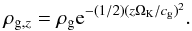 (1)It is natural to define the gas scale height hg as the one at which the gas density has decreased by a factor e compared to ρg, that of the mid-plane:
 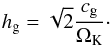 (2)We note that other choices are sometimes made in the literature. With this choice, the relation between the midplane density and the surface density is obtained by a simple vertical integration:
 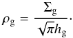 (3)A further simplification is to assume that the radial structure of the disk is described by power laws. Following Hayashi (1981) and Nakagawa et al. (1986), we adopt the following scaling laws for the so-called MMSN,
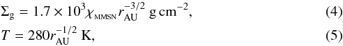 where rAU ≡ r/ 1 AU, and
  is a scaling factor on the density. The MMSN is a convenient representation of the planetesimal disk. It is based on the present-day observed planets and can therefore be considered representative of the last stages of the formation of the solar system at the time of the dispersal of the gas disk. It does not account for planetesimal-driven migration after the disk disperses. It is also less clear that is it a good representation of the gas disk (simulations of disk evolution generally yield different power laws both for Σg and T). However, the results of this work are easily scalable for any profile other than the MMSN.
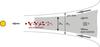 |
Fig. 1 Geometry of the problem considered in this study. The gas disk has a characteristic height hg and is accreting onto the star thus yielding a small but non-negligible inflow velocity. Dust particles grow by mechanisms not modeled in this study. They settle to the mid-plane and drift inward as a result of gas drag, at a pace set both by their size and the thermodynamical conditions in the gas disk. Their vertical extent is hd. Planetesimals are supposed to have formed preferentially near the star. They have sizes in the kilometer range or much larger and negligible inward drift. Their vertical extent hp is mainly governed by self-scattering. |
The values of a number of quantities of relevance to this work based on the MMSN scalings are presented in Appendix A. For the gas disk scale height, the following relation applies: 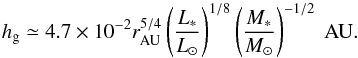 (6)The dust grains settle onto the midplane because of friction with the gas and the vertical component of the star’s gravitational force, yielding a sedimentation terminal velocity vz = −τsΩKz (Nakagawa et al. 1981). The sedimentation timescale is thus
 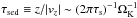 , i.e., it is proportional to the local Keplerian orbital timescale divided by the dimensionless stopping time τs (see Sect. 2.4 hereafter for the definition of τs). Except for the smallest particles, we can consider that dust has fully sedimented and has a scale height that is determined by its stopping time and turbulent stirring. Dubrulle et al. (1995) show that
 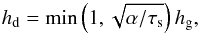 (7)where α is the traditional turbulence parameter(Shakura & Sunyaev 1973). (We note that Youdin & Lithwick (2007) extend this relation to any eddy mixing timescale with a slightly more complex dependence on τs which is minor and not taken into account here.) We will use a fiducial value α = 10-2 broadly compatible with measured T-Tauri accretion rates and disk observations (e.g., Hartmann et al. 1998; Hueso & Guillot 2005) and simulations of magneto-rotational instability in disks (e.g., Heinemann & Papaloizou 2009; Flock et al. 2013). We will also use a lower value α = 10-4 more relevant to the turbulence inside dead zones (e.g., Okuzumi & Hirose 2011). For the (compact) grains with sizes ranging from microns to tens of meters considered in this study, values of τs range between about 10-8 and 102 (see Fig. 3 hereafter for the correspondence between grain size and τs in the MMSN). With this value of the turbulence parameter, hd = hg for all grains smaller than about 1 cm at 1 AU and 0.1mm at 100 AU. For larger grains in the Stokes drag regime the scale height decreases inversely with the square root of the grain size.
The scale height of planetesimals is determined directly from their inclinations i:  (8)Inclinations are determined by the balance between excitation (scattering by planetesimals or density fluctuations in the gas disk) and damping (gas drag, tidal interactions with the disk and collisions). As discussed in the next section, damping is generally strong and eccentricities small (e~<0.05 for r< 10 AU; see Fig. 2). Eccentricities and inclinations are directly linked. For example, in the case of mutual scattering by planetesimals, i ~ e/ 2 (Ida & Makino 1992). On the basis of this approximation, at 1 AU and for 1000 km, we can expect hp ~ 5 × 10⁻³r, about an order of magnitude smaller than hg.
We can therefore expect that the geometry indicated by Fig. 1, i.e., hp ≤ hd ≤ hg, holds for all grains smaller than about 1 m at 1 AU and 0.1 mm at 100 AU. For larger grains the possibility that hp>hd is to be considered.
2.2. Sizes and eccentricities of planetesimals
Planetesimals will have a size distribution that will be affected both by accretion and destruction processes, by mechanisms leading to their formation and by gain and losses due to migration in the protoplanetary disk. In the present work, we will simply assume that their sizes are distributed between Rp,min and Rp,max. For simplicity, we use Rp,min = 1 km which roughly corresponds to the size below which the drift of the planetesimals must be taken into account. The maximum radius will depend upon accretion processes. Early in the evolution of the disk, streaming instabilities might provide an efficient way of making the first Ceres-sized (~500 km) planetesimals (Johansen et al. 2007). Subsequent growth must lead to Moon-sized objects and later to planetary mass objects.
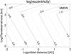 |
Fig. 2 Contour plot showing the decimal logarithm of the eccentricity as a function of planetesimal size and orbital distance for a standard MMSN disk model as obtained from an equilibrium between gas drag, tidal interactions, and excitation by a turbulent disk with a turbulence parameter γ = 5 × 10⁻⁴ corresponding to α = 10-2 (see Ida et al. 2008; Okuzumi & Ormel 2013). |
The eccentricities of planetesimals are excited by gravitational scattering by other planetesimals. As Ida et al. (2008) and Okuzumi & Ormel (2013) suggested, however, eccentricity excitation by density fluctuations of turbulence of the disk is comparable to or larger than that by planetesimal scattering, for usual values of α = 10-3 − 10-2 for magneto-rotational instabilities (MRI). We here consider the excitation by the MRI turbulence. While the excitation by scattering depends on the size distribution of planetesimals, the excitation by turbulence is independent of the size distribution of other planetesimals and also the size of perturbed planetesimals. The equilibrium eccentricities are given by a balance between the excitation and damping due to gas drag and tidal interactions. Ida et al. (2008) showed that the equilibrium eccentricities for small bodies, for which gas drag is dominant, are given by 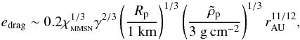 (9)where Rp and
  are the physical size and density of the perturbed bodies, respectively, and γ( <1) is a dimensionless parameter representing the strength of the turbulent stirring and is a function of the turbulence parameter α. We adopt the relation γ ≈ 5 × 10⁻⁴(α/ 10-2)1/2provided by Okuzumi & Ormel (2013) for ideal MHD. The equilibrium eccentricities for large bodies, for which tidal interactions is dominated, are then given by
 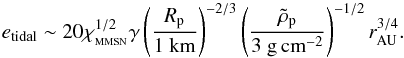 (10)The minimum of edrag and etidal is a value that is actually realized. (Given our fiducial value of α = 10-2, we use γ = 5 × 10⁻⁴.) In Fig. 2, we plot the equilibrium eccentricity as a function of Rp and r. The result shown in Fig. 2 predicts eccentricities that are very small at short orbital distances due to gas drag and higher at large orbital distances. Both small planetesimals and large ones have small eccentricities. This is due to gas drag for small objects and to dynamical friction for the large ones. We note that Fig. 2 is appropriate for MRI-active zones, but we expect much weaker turbulent stirring (∝α1/2) and therefore smaller eccentricities in dead zones.
As shown by Ormel & Kobayashi (2012), the gravitational stirring of planetary embryos starts to dominate over turbulent stirring when their mass becomes larger than ~0.3(α/ 10-2) M⊕. However, tidal damping is expected to dominate over self-stirring for the large embryos. The maximum eccentricity of large embryos is therefore expected to occur for the same masses/radii as in Fig. 2. We estimate a maximum scale height for these of hp/r ~ e/ 2, i.e., hp/r ~ 0.005(α/ 10-2)1/2 at 1 AU or hp ~ 0.1(α/ 10-2)1/2hg. For small values of α, viscous stirring sets a floor to the value of hp (Kokubo & Ida 2000). In any case, the largest objects in the size distribution are expected to have a scale height that is small compared to the gas scale height. In addition, hp decreases with decreasing Rp. Therefore, we simply adopt hp = 0.01hg as our standard choice for the scale height of the planetesimals. We experiment with other, more extreme ratios in Appendix E.
We note that when we consider small planetesimals in the presence large embryos, the former can be excited to greater heights (Kokubo & Ida 2002). Our calculations can easily be extended to the case of a size-dependent planetesimal scale height, but this would require a proper treatment of the evolution of the size distribution of planetesimals, which is beyond the scope of the present work.
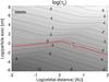 |
Fig. 3 Contour plot showing the decimal log of the dimensionless stopping time τs (see Eq. (21)) as a function of particle size and orbital distance for a standard MMSN disk model, α = 10-2, and assuming a physical density of particles |

2.3. Rate and geometry of gas accretion
The flow of gas in a disk is determined by the rate of angular momentum transport and the mass balance between inner and outer regions. In one dimension, the following equation for the mean velocity of the gas can be derived from the equations governing the spreading of a viscous disk (Lynden-Bell & Pringle 1974),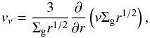 (11)where ν is the turbulent diffusion coefficient in the disk. For a MMSN-type disk with a uniform α, vν = 0 everywhere which is unrealistic (the disk spreads inward and outward at the same rate). When assuming Σg ∝ r-1, which is more commonly found in realistic disk evolutions (e.g., Hueso & Guillot 2005), vν = −(3/2)ν/r. The negative sign indicates an inward flow.
When considering the 2D structure of disks within the α-turbulence framework, it can be shown (e.g., Takeuchi & Lin 2002) that for most commonly used power-law relations for the density and temperature radial profiles, a meridional circulation sets in that maintains a strong, inward flow in the upper layers of the disk and a weaker outward flow in the mid-plane. The density-averaged flow still obeys Eq. (11)and is therefore generally inward. This has been advocated as the reason for the presence of chondrules and generally of grains having been formed near the protosun in the outer regions of the solar system (Ciesla 2009).
The presence of such a meridional circulation can lead to the retention in the disk of grains large enough to have settled to the mid-plane so that their outward motion compensates for the inward motion in the upper layers of the disk. Direct numerical simulations of magneto-rotational instability in protoplanetary disks by Fromang et al. (2011) failed to find such a circulation setting in, but the resulting flow was outward and not inward as was expected for an accretion disk, and the velocity fluctuations were found to be much larger than the mean flow, making the result more tentative. The problem hence still exists.
For simplicity, and without any pretention of capturing the detailed evolution of real disks we will assume hereafter vν ~ − ν/r.
2.4. Particle drift with accreting gas
We now rederive drift velocities for dust and planetesimals using the formalism of Adachi et al. (1976). These are widely available in the literature, but the expressions for the radial and azimuthal velocities are derived by assuming that the gas in the disk is at rest. The equation of motion of such a particle in a gas disk under the action of gas drag is 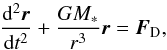 (12)where FD is the drag force vector per unit mass which is directed opposite to the velocity vector. Two regimes correspond to the case when the particles are smaller than the mean free path of the gas and the drag can be modeled by accounting for collisions of individual gas molecules (Epstein regime), and when the particles are larger and the gas must be modeled as a fluid. An expression for the amplitude of the drag vector that combines the two regimes (based on Adachi et al. 1976; Perets & Murray-Clay 2011) is
![Mathematical equation: \begin{equation} \FD= {\rho_\rmg\over \rhos s} \vth \vrel \min\left[1,{3\over 8}{\vrel\over \vth}\CD(Re)\right],\label{eq:FD} \end{equation}](/articles/aa/full_html/2014/12/aa23021-13/aa23021-13-eq88.png) (13)where
(13)where  is the mean thermal velocity and Re is the Reynolds number measuring the turbulence of the flow with a velocity vrel around a particle of diameter 2s and for a gas dynamic viscosity μg
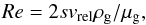 (14)
(14)
and CD is a dimensionless drag coefficient that is fitted semi-empirically as a function of Re (see Perets & Murray-Clay 2011):  (15)When Re ≪ 1 and using μg = ρgvthλg/ 2, it can be shown that Eq. (13) simplifies to the usual Epstein vs. Stokes relations:
  (16)Equation (12) can then be written in (r,θ) coordinates, assuming planar motions only and accounting for a radial velocity of the gas,
 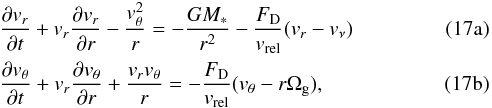 where rΩg = (1 − η)vK is the gas azimuthal velocity and
 ![Mathematical equation: \begin{equation} \vrel=\left[(v_r-v_\nu)^2+(v_\theta-r\Omega_\rmg)^2\right]^{1/2}. \end{equation}](/articles/aa/full_html/2014/12/aa23021-13/aa23021-13-eq103.png) (18)The η parameter is thus a relative measure of the departure of the gas azimuthal velocity from Keplerian. It can be shown to be directly related to the gas pressure gradient (Adachi et al. 1976):
(18)The η parameter is thus a relative measure of the departure of the gas azimuthal velocity from Keplerian. It can be shown to be directly related to the gas pressure gradient (Adachi et al. 1976):  (19)Following Adachi et al. (1976), we will assume that the azimuthal velocity difference between the gas and the particle is much smaller than the Keplerian azimuthal velocity, i.e., that δvθ ≡ vθ − vK ≪ vK. Furthermore we assume that the viscous drift velocity is also negligible, i.e., vν ≪ vK. Dropping all the second-order terms, Eqs. (17b) and (17a) then become
 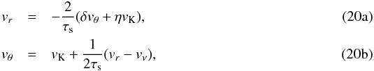 where we have introduced the stopping time,
  (21)It is then easy to derive the radial velocity and difference between azimuthal and Keplerian velocities of a particle of size s as
 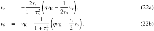 A simplification can be made by noticing that the gas velocity in the second equation will always be negligible. For small values of τs, the term is negligible over ηvK. For large values of τs, the azimuthal velocity becomes Keplerian so that δvθ → 0 anyway. We therefore simplify the above system of equations to
 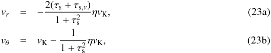 where we have introduced the critical stopping time below which the radial drift of a particle is mostly influenced by gas accretion in the disk:
  (24)Assuming an α prescription for the turbulent viscosity, we can approximate the inward radial velocity of the gas as:
  (25)so that the critical stopping time becomes
  (26)For the MMSN, τs,ν = 0.3α, independently of the orbital distance considered. At 1 AU, this implies that dust particles as large as 0.6 cm are dominated by the gas inflow for α = 10-3. Figure 3 shows the behavior of both τs and τs,ν as a function of orbital distance in the MMSN.
The relative velocity between the particle and the gas is, within the approximations made, independent of the viscous drift:  (27)Equations (13)–(15), (21), and (27)form a set of non-linear equations that, except in the Epstein and Re< 1 regime, must be solved iteratively.
2.5. The filtering length
In the simplest case, only the dust particles orbiting in the same plane as the planetesimal have a chance to hit it. We define 2b as the linear cross section of planetesimals. (For small planetesimals b ~ Rp.) If dust particles stayed at the same altitude in the disk, only a maximum fraction b/hd of the dust would possibly collide with planetesimals, the remaining  eventually being accreted by the star. However, particles are moved up and down by turbulence (for small particles) or by their own epicyclic motions (for large particles with τs~>1). Ciesla (2010) shows that the vertical location of small particles in a disk are governed by an advective-diffusive equation which can be modeled through a Monte Carlo approach,
 ![Mathematical equation: \begin{equation} z_i=z_{i-1}-(\alpha+\taus)\Omega_\rmK z \delta t + {{\rm Rnd}}\left[{2\over {\rm var}}\alpha h_{\rm g}^2\Omega_\rmK \delta t \right]^{1/2}, \end{equation}](/articles/aa/full_html/2014/12/aa23021-13/aa23021-13-eq129.png) (28)where zi and zi − 1 are the vertical location of a particle of dimensionless stopping time τs~<1 at two instants separated by δt and Rnd is a random number drawn from a distribution of variance var. The advection term (proportional to (α + τs)z) appears as a result of imposing hydrostatic equilibrium in the disk in the vertical direction. It prevents particles from drifting outside the disk. On the basis of simulations of magneto-rotational turbulence in disks, one expects that the particles receive kicks in velocity every
(28)where zi and zi − 1 are the vertical location of a particle of dimensionless stopping time τs~<1 at two instants separated by δt and Rnd is a random number drawn from a distribution of variance var. The advection term (proportional to (α + τs)z) appears as a result of imposing hydrostatic equilibrium in the disk in the vertical direction. It prevents particles from drifting outside the disk. On the basis of simulations of magneto-rotational turbulence in disks, one expects that the particles receive kicks in velocity every  . Using a Gaussian distribution for Rnd with var = 1, one can then show numerically that the characteristic time to cross the mid-plane for small particles is within 10%:
  . On the other hand, large particles cross the mid-plane at each orbit (e.g., Youdin & Lithwick 2007). Combining the two results yields a mid-plane crossing time
  (29)The timescale depends on the value of the turbulence parameter only for very small grains that have a scale height equal to the gas scale height. Otherwise, the smaller particle scale height compensates for the added turbulent mixing. Large particles undergo epicyclic motions and their settling is independent of turbulence.
We can then use Eqs. (23a)and (29)to calculate a filtering length, which is the length after which most grains, regardless of their initial positions, have crossed the mid-plane:  (30)We thus obtain
  when τs~<α,
  when 1~>τs~>α, and λf/r ~ (2 /τs)η when τs~>1. For the smallest particles, we can expect that λf/r< 10-4, a very small filtering length. Even for the fastest drifting particles, for which we expect hp ~ hd anyway, λf/r~<4η ~ 8 × 10⁻³.
This implies that even in the case of rapidly drifting particles, turbulence in the disk should ensure that particles always have the opportunity of encountering planetesimals in the mid-plane. In other words, if enough planetesimals are present, perfect filtering can occur, i.e., there may be cases for which the star can accrete dust-free gas.
3. Filtering in the geometrical limit
3.1. 2D collision probabilities
We will now derive the rate of impact of drifting dust onto a non-drifting planetesimal on a circular orbit in the geometrical limit (i.e., neglecting gravitational focusing). In two dimensions, this impact rate is the product of the planetesimal linear cross section b and the encounter velocity Δvcol:  (31)The mass accretion of dust by planetesimals is then Ṁp = ℛΣd.
The velocity difference between the planetesimal and the particle calculated assuming that they do not interact is  (32)where vr and vθ are the particle radial and azimuthal velocities defined by Eqs. (23a)and (23b)and Vr and Vθ are those for the planetesimal. We assume that τs,ν ≪ 1. For non-drifting planetesimals on circular orbits, Vr = 0 and Vθ = vK thus yielding
  (33)In the geometrical circular limit, b = Rp and Δvcol = Δvcirc, i.e., we neglect any interaction resulting from e.g., gravitational focusing (see below). The impact rate in this limit is then
  (34)When
  , this expression is equivalent to Eq. (22) of Ormel & Klahr (2010) who derive this impact rate by an analysis of the trajectory of dust particles.
The 2D probability that a planetesimal will accrete a given dust grain is then given by the ratio between the mass accreted Ṁp and the global mass flow of dust grains past the planetesimal 2πrvrΣd,  (35)In the geometrical limit, this can be shown to yield1
 (36)The probability thus decreases from a maximum value ~Rp/ (2πrτs,ν) for low values of τs when the drift is controlled by the gas flow to a minimum value of Rp/ (πr) for large dust particles. For small particles, the high probability is due to the dust and the planetesimal having very different azimuthal speeds. For large particles, the azimuthal and radial velocity difference between dust and planetesimal is small so that only the dust located at the right azimuth will collide with the planetesimal. We note that the probability remains finite for τs → ∞, i.e., for non-drifting dust. Indeed, Eq. (36)is time-independent: it yields the probability of collision in the limit of infinite time. This view is thus complementary to that obtained by using collision rates to estimate planetesimal growth timescales.
3.2. 3D collision probability
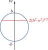 |
Fig. 4 Sketch showing how the linear cross section of an assumed spherical planetesimal varies as a function of the impact distance w, given a maximum (equatorial) cross section 2b. |
We have so far considered cases when dust and planetesimals orbit in the same plane. In reality, the 3D nature of the disks discussed in Sect. 2.1 must be considered. As in the 2D case, the collision rate is a product of a linear cross section to a collision velocity, but this time, as shown in Fig. 4, the linear cross section depends on w, the impact parameter of the dust. The mass accretion rate can thus be calculated by integrating over all impact parameters and all positions of the planetesimal on its trajectory, accounting for variations of the dust density and of the collision velocity,  (37)where both Δvcol, r and z are functions of the mean anomaly ℳ. We simplify the integration by assuming that we can neglect the variations of ρd along the trajectory of the planetesimal (i.e., the values of ℳ) and that we can calculate a mean collision velocity:
  (38)The accretion rate can then be written as an integral over the cross section of the planetesimal:
 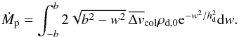 (39)It may seem strange to neglect the variations of ρd along the trajectory of the planetesimal and not over its cross section. However, it will enable us to link the 2D solutions obtained in the previous section to the 3D ones.
It turns out that the above integral may be expressed in terms of a sum of modified Bessel functions of the first kind I0 and I1: ![Mathematical equation: \begin{equation} \dot{M}_\rmp=\pi \bcol^2 \vmeancol\rho_{\rm d,0} {\rm e}^{-\bcol^2/2\hdust^2}\left[I_0\left(\bcol^2\over 2\hdust^2\right) +I_1\left(\bcol^2\over 2\hdust^2\right)\right]\cdot \end{equation}](/articles/aa/full_html/2014/12/aa23021-13/aa23021-13-eq182.png) (40)We recover the 2D case when b ≫ hd, in which case
(40)We recover the 2D case when b ≫ hd, in which case 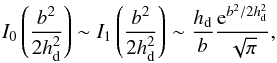 which implies that
 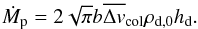 Given that
  , we indeed obtain
  (41)In the more natural case when b ≪ hd, then
  and
and  so that
  (42)We will hereafter assume that this hypothesis is true most of the time. When the dust disk is thinner than the planetesimal disk, we will also assume that the relation remains valid but with hd replaced by the corresponding scale height for planetesimals, hp.
A simplified relation between the 3D and 2D collisions probabilities is hence: ![Mathematical equation: \begin{equation} {\cal P}={\rm min}\left[1,{\sqrt{\pi}\over 2}{\bcol\over {\rm max}\left(\hdust,h_\rmp\right)}\right] {\cal P}_{\rm 2D} . \label{eq:P3D} \end{equation}](/articles/aa/full_html/2014/12/aa23021-13/aa23021-13-eq192.png) (43)Given our choice for the expression of hg and hence hd, there is a factor
(43)Given our choice for the expression of hg and hence hd, there is a factor  mismatch with the expressions assumed by Ormel & Klahr (2010) and Ormel & Kobayashi (2012). We note that hg and hd may be defined arbitrarily, so that it is natural that a factor on the order of unity appears next to the b/hd ratio.
In the analytical derivations hereafter, we will assume for simplicity that  . However in the numerical calculations and plots we will assume hp = 0.01 hg, which will limit the accretion probability of boulders larger than several meters. (We note that in the limit that hp<hd, Eq. (43)is independent of hp.)
In the geometrical, circular limit (i.e., b = Rp) and for small-enough dust such that hd> (2/ , we obtain
 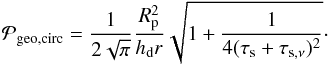 (44)This probability thus depends on size of the planetesimals and properties of the dust (thickness of the dust disk and stopping time). Both the thickness of the dust disk (Eq. (7)) and the quantity τs,ν (Eq. 26) are directly dependent on the value of the turbulence parameter. We can thus write the probability in terms of the gas (instead of the dust) scale height and further condense the notation,
 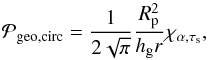 (45)where
  (46)It is useful to approximate this last quantity depending on the stopping time of dust particles and turbulent viscosity parameter, using the fact that for the MMSN scaling, τs,ν ≈ 0.3α:
 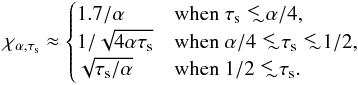 (47)When leaving aside very large particles (governed by different relations), the value of χα,τs ranges from 1.7 /α to its lowest value 1/
 for τs = 1/2 particles. The 1.7 /α value for small particles is determined entirely by the (mean) gas advection rate. The 1/
 dependence, however, relates to the ability of particles to be lofted by turbulence.
3.3. Planetesimal size distribution and filtering mass
We now look for the mass in planetesimals that is required for an efficient filtering of dust grains at any location. If we assume a single size Rp for all planetesimals (monodisperse size distribution), then we only have to obtain NRp the number of planetesimals of that size such that  and obtain the total mass from
 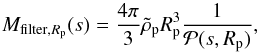 (48)where Mfilter,Rp(s) is thus the mass in planetesimals of size Rp that is required to efficiently filter dust of size s. In the geometrical circular regime, this may be approximated as
 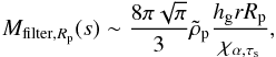 (49)where χα,τs takes the values defined in Eq. (47)depending on α and τs. In this limit, the filtering mass is therefore linearly proportional to the size of the planetesimals considered. Larger planetesimals have a larger cross section individually, but a smaller collision probability collectively yielding a larger filtering mass.
Of course, planetesimals in the protoplanetary disk will not all be the same size. Instead, we envision that their size distribution is defined by a power law,  (50)where N is the number density of planetesimals of size Rp and A is a constant defined by the total number of planetesimals, N0 = ∫AR− qdR. We therefore calculate the mass in planetesimals of all sizes required to capture all incoming dust grains of size s as
  (51)where
  is given by Eq. (43).
A collisional cascade yields a size distribution characterized by q ~ 7/2 (Tanaka et al. 1996). (This corresponds to a mass distribution  .) For comparison, the size distribution in the asteroid belt is characterized by q ≈ 4 for asteroids with radii above 70 km, and q ≈ 2.5 for smaller asteroids (e.g., Morbidelli et al. 2009). For simplicity, we adopt q = 7/2 by default. In the geometrical circular limit, we then obtain
  (52)where
  (53)It is easy to show that Rp,mean = Rp,min if q ≫ 4, Rp,mean = Rp,max if q ≪ 3 and for q = 7/2,
  .
.
For the MMSN, this translates into 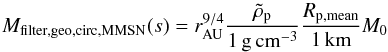 (54)with
 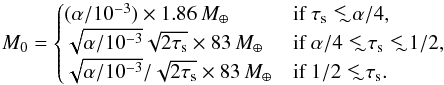 (55)These estimates show that even with very small planetesimals, efficient filtering requires very large masses in the geometrical limit. Small grains appear to be easier to filter, but this does not include the hydrodynamical effects which tend to drastically suppress accretion. Conversely, the estimates do not include possible focusing for large mass planetesimals and/or dust.
3.4. Filtering efficiency
We now want to estimate the fraction of dust that is effectively filtered by the planetesimals and its complement, the fraction of dust that passes through the planetesimal belt and is accreted by the star. For simplicity we will assume that collisions effectively lead to accretion, although the reality may be different. We consider Np(Rp,r)dRpdr, the number of planetesimals with sizes between Rp and Rp + dRp, and at orbital distances between r and r + dr. We define the disk-integrated filtering efficiency for dust of size s as 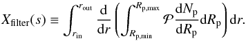 (56)Using the distribution of planetesimal sizes defined by Eq. (50)and the surface density of planetesimals Σp(r), the disk-integrated filtering efficiency can be written in the form
  (57)where xfilter(s,r) is the characteristic filtering efficiency for dust of size s at orbital distance r,
  (58)where Mfilter is defined by Eq. (51). The quantity xfilter thus measures the filtering efficiency at each orbital distance, allowing us to estimate where the dust is mostly absorbed.
In the geometrical, circular limit, Eq. (52)leads us to  (59)Replacing Σp and hg by their MMSN scaling relations yields the filtering efficiency of a swarm of planetesimals with the same total mass as the present solar system:
  (60)Integrating over orbital distances, and assuming that rin ≪ rout yields
  (61)These equations show that, in the geometrical circular limit, perfect filtering (i.e., Xfilter,geo,circ,MMSN ~ 1) by a MMSN disk of solids is only possible close to the star, for small particles, and/or weak turbulence (keeping in mind that χτs,α is between 1 /α for small particles and 1/ for larger ones), and by a swarm of very small planetesimals dominated by km-sized planetesimals. This is shown in Fig. 5 for two values of α: the filtering efficiency in the geometrical circular limit is minimum for τs ~ 1, and increases both for larger and smaller particle sizes. As shown by the dashed curves in Fig. 5, if gas advection by the accreting disk could be neglected (χτs,α ~ 0), the filtering efficiency would increase steadily for smaller dust particles because of their very slow migration which increases the probability of hitting a planetesimal. However, gas advection forces small particles to move at a rate which prevents this increase: the filtering efficiency then becomes independent of the size for particles such that τs~<α.
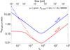 |
Fig. 5 Filtering factor by an MMSN disk of planetesimals of size Rp,mean = 1 km and density |
This demonstrates that an efficient filtering of dust particles is difficult to achieve at least in the geometrical, circular limit, even with a mass of planetesimals equivalent to the MMSN, which likely represents the maximum available limit, at least for the solar system. Importantly, the filtering efficiency is inversely proportional to planetesimal density and size, implying that it is most effectively done by small and/or porous planetesimals. It is also proportional to the surface density of planetesimals which is generally thought to be a strong function of orbital distance, implying that filtering is most effective close to the star.
However, we must consider additional processes arising in real disks.
4. Filtering: additional effects
4.1. Accounting for eccentric orbits
Following Ormel & Klahr (2010), we have so far only considered planetesimals with circular orbits. In this case, the relative motion between the planetesimal and the dust results from the combination of the difference in azimuthal velocity of the planetesimal (Keplerian) and of the dust (sub-Keplerian) and the small radial drift velocity of the dust. For the more general case of planetesimals on eccentric orbits, the encounter velocities are generally much larger because of the non-zero radial velocity of the planetesimals themselves. A detailed solution of the problem is complex (see Kary & Lissauer 1995). We provide instead a simplified treatment.
We now consider the encounter of a dust grain at orbital distance r with a planetesimal with eccentricity e and true anomaly νp. Its semi-major axis a is thus such that a(1 − e2) = r(1 + ecosνp), and its radial and azimuthal velocities are, respectively, 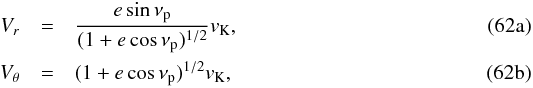 where vK is the Keplerian velocity at r.
The encounter velocity between the dust grain and the eccentric planetesimal is now obtained by calculating Δvr = vr − Vr and Δvθ = vθ − Vθ, ![Mathematical equation: % subequation 2842 0 \begin{eqnarray} {\Delta v_r\over v_\rmK} &=&-{2(\taus+\tausnu)\over 1+\taus^2}\eta - {e\sin\nu_\rmp\over (1+e\cos\nu_\rmp)^{1/2}} ,\label{eq:Deltavr}\\ {\Delta v_\theta\over v_\rmK} & =& -{1\over 1+\tau_\rms^2} \eta -\left[(1+e\cos\nu_\rmp)^{1/2}-1\right] , \label{eq:Deltavtheta} \end{eqnarray}](/articles/aa/full_html/2014/12/aa23021-13/aa23021-13-eq272.png) where we have neglected variations of τs and η with r. The instantaneous accretion rate is still calculated as Eq. (34), but because it is now time dependent, we integrate over the planetesimal’s orbit,
where we have neglected variations of τs and η with r. The instantaneous accretion rate is still calculated as Eq. (34), but because it is now time dependent, we integrate over the planetesimal’s orbit, 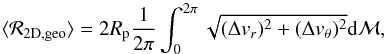 (64)where the variations of Σd over the planetesimal’s orbit have been neglected and the integral is performed over all mean anomalies ℳ (νp is calculated as a function of ℳ using Kepler’s equation).
When performing the integral, Δvr and Δvθ both contain a constant part and a variable part proportional to the planetesimal’s eccentricity. Because this variable part is proportional to esinνp and ecosνp, respectively, its contribution is either positive or negative. If its amplitude is smaller than that of the constant part, we can expect it to average out to a negligible amount. If, however, its amplitude is larger than the constant term, because of the square function, it will eventually become dominant. This will occur when 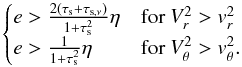 (65)Both conditions must be met, and since the first one is more important for τs> 1 and the second one for τs< 1, we can equivalently distinguish the circular and eccentric regimes by comparison of e to the critical eccentricity
 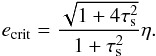 (66)When e<ecrit, the eccentricity term has both positive and negative contributions (sinνp and cosνp change sign) and can be considered as averaging out to negligibly small values. When e ≫ ecrit, the eccentricity term dominates so that both positive and negative values of sinνp and cosνp lead to an increase in the accretion probability. For this case, the mean accretion rate can be written
 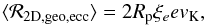 (67)where we have defined
 ![Mathematical equation: \begin{eqnarray} \xi_e=\int_0^{2\pi} {1\over e}\left\{ {\left( e\sin \nu_\rmp \right)^2\over 1+e\cos\nu_\rmp} +\left[\sqrt{1+e\cos\nu_\rmp}-1\right]^2 \right\}^{1/2} {\rm d}{\cal M}. \label{eq:xie} \end{eqnarray}](/articles/aa/full_html/2014/12/aa23021-13/aa23021-13-eq289.png) (68)The value of ξe can be calculated by solving Kepler’s equation and is only a function of the eccentricity of the object considered. It is shown in Fig. 6. For small eccentricities e~<0.2 we obtain ξe ≈ ξe(e = 0) = 0.743, a value that we adopt from now on.
(68)The value of ξe can be calculated by solving Kepler’s equation and is only a function of the eccentricity of the object considered. It is shown in Fig. 6. For small eccentricities e~<0.2 we obtain ξe ≈ ξe(e = 0) = 0.743, a value that we adopt from now on.
Combining the low-eccentricity and high-eccentricity limits, the average encounter velocity can be calculated from the quadratic mean of Eqs. (63a) and (63b) (and assuming τs,ν ≪ 1) 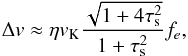 (69)where the eccentricity factor fe is calculated as:
 ![Mathematical equation: \begin{equation} f_e= \sqrt{1+\left[\xi_e \frac{1+\taus^2}{\sqrt{1+4\taus^2}} {e\over \eta}\right]^2}\cdot\label{eq:fe} \end{equation}](/articles/aa/full_html/2014/12/aa23021-13/aa23021-13-eq295.png) (70)Dropping the mean terms, we thus write the mean accretion rate
(70)Dropping the mean terms, we thus write the mean accretion rate  (71)and the average collision probability as
  (72)The behavior of fe as a function of dust size is shown in Fig. 7. The diagram of course resembles the contour plot obtained for eccentricities (see Fig. 2). The eccentricity factor will become important for large planetesimals and at large orbital distances, i.e., when the gas drag is reduced. Quantitatively, when a planetesimal eccentricity e = 0.01 we obtain fe ≈ 4.25 for small dust particles. When plotted as a function of τs (not shown here), the eccentricity factor is found to be small and flat for small values of τs. A small drop occurs for τs = 1/
 , but the eccentricity factor then rapidly increases and becomes proportional to τs because for large pebbles and boulders, the relative motions between particles and planetesimals due to gas drag become small. Eccentricity effects then play a dominant role in these encounters.
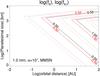 |
Fig. 7 Contour plot of the decimal logarithm of the eccentricity focusing factors fe (see Eq. (70)) (in black) and fe,i (see Eq. (78)) (in red) as a function of orbital distance in a MMSN disk for dust of 1 mm in size. The eccentricity is the same as in Fig. 2. |
The difference between these the two low- and high-eccentricity regimes can be understood by calculating the ratio Γ of the time for the dust to drift from the apocenter to the pericenter divided by half of the orbital period of the planetesimal:  (73)It is easy to show using Eq. (23a) that
  (74)Thus for τs ≫ 1, e = ecrit correspond to Γ = 2 /π. When Γ < 1, dust grains generally have only one possible encounter with the planetesimal on its orbit and thus the collision probability defined by Eq. (72) is very close to that obtained for a planetesimal on a circular orbit. Conversely, when Γ ≫ 1, the drifting dust has many possibilities of colliding with the eccentric planetesimal, thus increasing the collision probability proportionally to the number of encounters. For τs ≪ 1 however, the multiple encounters are balanced by a collision geometry which is less favorable for collisions so that a higher eccentricity is required for the collision probability to become proportional to eccentricity.
4.2. Including inclinations
We have seen in the 2D case that eccentricity may help collisions. However, as discussed in section 2.1, both eccentricities and inclinations are expected to be excited, with i ~ e/ 2. It is thus important to also consider inclined orbits in the calculation of collision probabilities.
Adapting Eqs. (63a)and (63b)to the 3D case, and neglecting variations of the gas and dust velocity with height in the disk (see Takeuchi & Lin 2002), we can express the approach velocities between an inclined planetesimal and dust as ![Mathematical equation: % subequation 3203 0 \begin{eqnarray} {\Delta v_r\over v_\rmK} &=&-{2(\taus+\tausnu)\over 1+\taus^2}\eta - {e\sin\nu_\rmp\over (1+e\cos\nu_\rmp)^{1/2}} ,\label{eq:3Deltavr}\\ {\Delta v_\theta\over v_\rmK} & =& -{1\over 1+\tau_\rms^2} \eta -\left[(1+e\cos\nu_\rmp)^{1/2}\cos i-1\right] , \label{eq:3Deltavtheta}\\ {\Delta v_z\over v_\rmK} & =& -(1+e\cos\nu_\rmp)^{1/2}\sin i. \label{eq:3Deltavphi} \end{eqnarray}](/articles/aa/full_html/2014/12/aa23021-13/aa23021-13-eq312.png) The approach velocity
The approach velocity  can be approximated by retaining only the leading squared terms:
 ![Mathematical equation: \begin{eqnarray} \left({\Delta v\over v_\rmK}\right)^2&\approx &{4\taus^2+1\over (1+\taus^2)^2}\eta^2\nonumber \\ &&+e^2\left[{\sin^2\nup\over (1+e\cos\nup)^2}+{1\over 4}\cos^2\nup\right]+2(1-\cos i). \end{eqnarray}](/articles/aa/full_html/2014/12/aa23021-13/aa23021-13-eq314.png) (76)By averaging approximately over the mean anomalies we then obtain
(76)By averaging approximately over the mean anomalies we then obtain  (77)where the eccentricity-inclination factor fe,i is calculated as
  (78)These relations thus replace Eqs. (69)and (70). Given that i ~ e/ 2, and ξe ≈ 0.743, the inclusion of inclination effects thus leads to approach velocities which are about 50% higher than when considering eccentricities alone (see Fig. 7).
4.3. Gravitational focusing
For large-enough planetesimals, gravitational focusing must be taken into account. Given the complex behavior of the three-body problem and the added complexity of gas drag, this can become a challenging problem requiring detailed numerical integrations. Here, we follow Ormel & Klahr (2010) in deriving simplified expressions for the focusing factor ffocus in three regimes: (1) in the settling regime, gas drag is the dominant mechanism controlling the trajectories of small particles around sufficiently large planetesimals; (2) in the Safronov regime, gravitational effects dominate over gas drag and lead to the classical gravitational focusing; (3) in the three-body regime, the interaction of (large) particles and (large) planetesimals must include the global geometry of the problem and the presence of the central star and leads to much more complex effects.
For simplicity, we will not account for eccentric and/or inclined orbits when calculating the enhancement of the collision probability due to gravitational focusing. First, this is a complex problem, beyond the scope of the present paper. Second, the increased cross section of eccentric planetesimals is generally matched with a larger encounter velocity so that the collision probability is often close to that of a planetesimal on a circular orbit. Last, in any case, planetesimal orbits are expected to have a range of eccentricities from circular to the maximum eccentricity so that the effect of eccentricity and gravitational focusing may be decoupled.
Because we will consider gravitational effects, it is useful to define the ratio of the planetesimal to the stellar mass  (79)and the Hill radius
  (80)The Bondi radius will become important in the settling regime. Following Lambrechts & Johansen (2012), we define it as a function of the dust-planetesimal encounter speed Δv,
  (81)For small enough dust particles with τs~<1, Eq. (69)Δv becomes independent of the dust size and RB depends only on the planetesimal properties2.
Using Δv ≈ ηvK, one can show that the minimum size for a planetesimal to have a Bondi radius larger than the planetesimal size is  (82)where
  and R∗ are the central star’s mean density and radius, respectively. For
  and our prescriptions for an MMSN-like disk,
  km independently of the orbital distance.
For larger planetesimals, an important limit is the size at which the Bondi radius equals the Hill radius. This occurs for 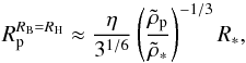 (83)implying
 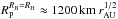 with the same fiducial planetesimal density.
4.3.1. The settling regime
 |
Fig. 8 Illustration of dust capture in the settling regime. Planetesimals with a radius Rp between about 100 km and 1000 km have a Bondi radius larger than Rp but smaller than the Hill radius (see text). For the critical stopping time |

For small particles (with τs~<1) the effect of gas drag can combine with the gravitational pull of the planetesimal to increase the collision cross section, as illustrated in Fig. 8. We consider the case where planetesimal and dust approach each other with an initial velocity Δv0. Because we only consider small particles with τs~<1, we approximate the dust to planetesimal velocity difference as ηvK. However, because of the increase in the capture cross section we also have to account for the Keplerian shear. The planetesimal being at an orbital distance r and the dust particle being initially at r + b0, by assuming b0/r ≪ 1 we obtain 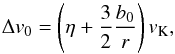 (84)where b0 is the initial impact parameter. The change in velocity δv of the dust particle in the reference frame of the planetesimal can be estimated by multiplying the gravitational acceleration from the planetesimal to the stopping time of the particle,
  (85)We expect the capture cross section in the settling regime to correspond to the impact parameter for which δv is on the order of the initial approach velocity Δv0. In the limit of τs ≪ 1 it can be shown that the condition for settling is δv ~ Δv0/ 4, which Ormel & Klahr (2010) then adopted for all τs.
By combining these equations, we derive a cubic equation that defines the impact parameter for collisions b0:  (86)This equation, which has one real positive root, is the same as that of Ormel & Klahr (2010).
For large values of τs we obtain b0 ~ (8τs)1/3RH. This equation hence implies that the impact parameter should increase indefinitely with τs, simply because Eq. (85)predicts a velocity change that also increases with τs. In reality, this remains true only up to the point when the stopping time and interaction time b0/ Δv0 become comparable. As noted by Lambrechts & Johansen (2012), this corresponds to the point when the impact parameter equals the Bondi radius. Particles with larger stopping times tend to be more easily gravitationally scattered and the effective planetesimal cross section to capture them decreases accordingly. This critical stopping time  and corresponding impact radius
  are linked by
  (87)Using Eq. (85)and δv ≈ ηvK/ 4 (neglecting shear this time), we obtain for the critical stopping time:
  (88)This may be also written in terms of the Hill and Bondi radius of the planetesimal:
  (89)Using Eqs. (87), (88), and (81), one can show that
  .
.
In order to link the weak and strong coupling regimes and reproduce numerical results, Ormel & Kobayashi (2012) propose the fit 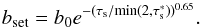 (90)Figure 9 shows how the effective cross section in the settling regime bset changes as a function of the stopping time and of the size of the planetesimal (measured in terms of the ratio
  ). The results for small planetesimals (RB/RH~<1) are very similar to Lambrechts & Johansen (2012, see their Fig. 4) and are almost independent of planetesimal size: The maximum settling cross section is obtained for
  and is equal to the Bondi radius of the planetesimal for the prescribed encounter velocity. For larger planetesimals with a Bondi radius larger than the Hill radius, the increase in cross section is suppressed because of the Keplerian shear. (We note that the minimum for
  in Eq. (90)corresponds to RB = 0.9RH.) A detailed study of the consequences of Eqs. (86)and (90)on the form of the solutions is presented in Appendix C.
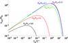 |
Fig. 9 Value of the effective capture radius bset in units of the Bondi radius rB as a function of the ratio of the stopping time of the dust particle to the critical stopping time |

The encounter velocity for the settling regime is obtained directly from Eqs. (90)and (84):  (91)The focusing factor for the settling regime is then obtained by dividing the new collision rate 2bsetΔvset by the geometrical rate 2RpΔv:
  (92)
(92)
4.3.2. The Safronov regime
When planetesimals are small enough so that their gravitational reach is not affected by stellar tides, and the settling effect from Sect. 4.3.1 is not important, the impact parameter is given by the well-known Safronov (1972) relation:  (93)where Δvcirc is defined by Eq. (33). This relation, however, fails in the limit when gas drag becomes important, both in the settling regime described previously and in the hydro regime to be explained next. This occurs when the stopping time τs becomes smaller than the time required to cross the planetesimal Hill sphere, τH = ΩKRH/ Δvcirc . Taking into account such an effect for small τs, we set the focusing factor in the Safronov regime as:
  (94)The corresponding impact parameter is
  . The added factor ensures that the focusing factor has the usual form when τs ≫ τH, while it becomes smaller than one when gas drag becomes significant (τs ≪ τH) outside of the validity range of Eq. (93). In this case the impact parameters are given by the expressions for the geometric, settling, or hydro regimes instead3.
4.3.3. The three-body regime
For large particles (τs> 1) around large planetesimals, both the gravity of the planetesimals and of the central star must be taken into account. This leads to a much more complex behavior including the presence of horseshoe orbits and the fact that only particles with specific impact parameters can enter the planetesimals’ Hill sphere.
The approach velocity derived from three-body numerical integrations without gas drag is (Ormel & Klahr 2010)  (95)whereas the impact rate is:
 ![Mathematical equation: \begin{equation} b_{\rm 3b}=\left(1.7\sqrt{R_\rmp R_\rmH}+R_\rmH/\taus\right){\rm e}^{-\left[0.7(\eta/\taus)(r/R_\rmH)\right]^5}. \end{equation}](/articles/aa/full_html/2014/12/aa23021-13/aa23021-13-eq376.png) (96)This second equation is based on Eq. (31) from Ormel & Klahr (2010), but multiplied by an exponential factor to account for gas drag and better reproduce the results of numerical models (Ormel & Kobayashi 2012). Using Eqs. (31), (33), (34), and (80), we write the focusing factor in the three-body regime as
(96)This second equation is based on Eq. (31) from Ormel & Klahr (2010), but multiplied by an exponential factor to account for gas drag and better reproduce the results of numerical models (Ormel & Kobayashi 2012). Using Eqs. (31), (33), (34), and (80), we write the focusing factor in the three-body regime as ![Mathematical equation: \begin{eqnarray} f_{\rm 3b}&= &{1\over \eta}{1+4\taus^2\over \sqrt{1+4\taus^2}}\nonumber \\ &&\times3.2\left[\left(\mup \Rp r\right)^{1/2}+{0.5\over \taus}\mup^{2/3} r\right]{\rm e}^{-(\eta \mup^{-1/3}\taus^{-1})^{5}}. \end{eqnarray}](/articles/aa/full_html/2014/12/aa23021-13/aa23021-13-eq377.png) (97)
(97)
4.3.4. The gravitational focusing factor
Following Ormel & Kobayashi (2012), we write  (98)The value of ffocus is thus calculated from the focusing factors in the different regimes, with 1 indicating a geometrical regime. Based on this determination, we assess the impact radius and the encounter velocity:
 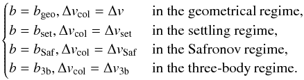 (99)Figure 10 shows how values of ffocus change as a function of dust and planetesimal sizes, assuming planetesimals on circular orbits. For small planetesimals (
 100 km) and dust sizes such that τs~<1 (corresponding to about 1 m at 1 AU), the focusing factor is very close to one, meaning that the accretion probability is defined by the geometric probability. For larger sizes, gravitational effects begin to dominate and lead to very high values of ffocus. In this diagram, most of the area is dominated by collisions in the geometric and Safronov regimes. For planetesimals above 100km, the encounters with dust mostly take place in the settling regime, in which the gravitational pull of the planetesimals, which tends to increase the collision probability, is strongly suppressed by the gas drag. By comparison, three-body collisions play a role only when considering large particles and they will thus only play a limited role here.
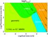 |
Fig. 10 Contours of the logarithm of the gravitational focusing factor log 10(ffocus) (see Eq. (98)) as a function of dust size (in cm) and planetesimal size (in km), at 1 AU in the MMSN. The physical density of dust and planetesimals is set to 1 and 3 g cm-3, respectively. The different physical regimes (geometric, Safronov, settling, three-body) are identified by different colors. This figure assumes that planetesimals are on circular orbits. |
4.4. Hydrodynamical effects
4.4.1. The hydrodynamical flow
 |
Fig. 11 Illustration showing how gas streamlines (in black) are deflected around the planetesimal (at the center). The red streamlines correspond to dust particles with a stopping time that is on the same order as the interaction timescale. The thick red lines correspond to the most extreme streamlines leading to a collision, which define bhydro(τs). |
It is important to notice at this point that the collision probability thus derived is valid in the limit that the hydrodynamic flow of gas around the planetesimal can be neglected. As shown by Sekiya & Takeda (2003) and illustrated in Fig. 11, this is not the case for small dust particles. More specifically, these authors show that a dust particle will be carried by the flow around the planetesimal if the dust particle stopping time is on the same order as or smaller than the planetesimal crossing time. This problem is well-known in the geophysical context where it affects, for example, the ability of rain drops and snow flakes to collect aerosols (e.g., Feng 2009).
We define a non-dimensional friction parameter τf which is the ratio of these two timescales,  (100)where Δv is the velocity of the flow during the encounter as determined by Eq. (69)(taking possible eccentric orbits into account).When τf ≪ 1, dust particles have a stopping time that is much shorter than the gas interaction time; they rapidly adjust their velocity vector to follow the gas and we thus expect accretion to be inefficient. Conversely, when τf ≫ 1, the particles’ stopping time is too long and we expect hydrodynamical effects to be negligible for the calculation of the collision probability. The numerical simulations by Sekiya & Takeda (2003) (see also Feng 2009; Sellentin et al. 2013) show that the collision probability drops when τf~<1, and it actually becomes consistent with zero in the simulations they present when τf~<0.3.
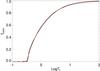 |
Fig. 12 Value of fhydro as a function of the dimensionless friction time τf as obtained by Sekiya & Takeda (2003, their Fig. 8) (black line) and our fit (red line and Eq. (105)). |
We write the reduction factor on the collision probability due to this factor fflow. From fitting the numerical simulations of Sekiya & Takeda (2003) as shown in Fig. 12, we obtain  (101)This factor tends asymptotically to 1 for large values of τf and it drops to zero when τf~<0.3. (The fact that it becomes negative is not important as it will be taken care of in the next section.)
4.4.2. The boundary layer
When the flow factor becomes too small, one must account for the boundary flow and for the fact that a small fraction of the particles with the right impact parameter will hit. The size of the boundary layer can be written (Wurm et al. 2004)  (102)where qboundary can be seen as either the flow velocity inside a porous planetesimal (Wurm et al. 2004) or as the flow velocity difference between the dust particles and the gas (Sekiya & Takeda 2005). We use the latter approach to calculate qboundary based on the kinematic theory of gases, which yields
  (103)where CD is the drag coefficient from Eq. (15)and φ is the porosity of the planetesimal. It can thus be seen that even non-porous bodies with φ = 0 will have non-zero qboundary flow. (We will assume φ = 0, but retain it in the equations for reference.)
Because this concerns small particles, it is useful to consider the behavior of this boundary layer in the Epstein regime, in which case Eq. (102) takes a simple form  (104)Given that CD is on the order of unity for the relevant Reynolds numbers and that
  is tiny, the boundary layer is generally very small. The reduction factor to be applied to particles with τf~<0.3 is thus on the order of 10-6 in most cases.
4.4.3. The hydrodynamical factor
This suppression of accretion is expected to occur in the hydrodynamical regime but not in the settling regime because of the slow encounters. In the settling regime, the particle is dragged towards the planetesimal. Once this process starts, it is irreversible because the gravitational pull of the gravitating body steeply increases. The outcome does not depend on the physical size (cross section) of the body as it does in the Safronov regime and it should not depend on the precise flow pattern in the vicinity of the body. As an illustration, the recent calculations by Ormel (2013) show that a protoplanet (or big planetesimal) strongly affects the gas flow around it, yet can still accrete particles at large cross sections when the interactions take place in the settling regime. This implies a steep jump in the accretion rate as the particle transitions from the Safronov/hydrodanamic regime to the settling regime. Further work is needed to understand the details of this transition, which we omit here for simplicity.
In summary, if the settling regime does not apply, the hydrodynamical correction factor is given by ![Mathematical equation: \begin{equation} f_{\rm hydro}=\max\left[\left({3\over 8}{C_{\rm D}\over 1-\phi}{s\over R_\rmp}{\vcol\over c_\rmg}\right)^{1/2},1-0.42\tauf^{-0.75}\right]. \label{eq:fhydro} \end{equation}](/articles/aa/full_html/2014/12/aa23021-13/aa23021-13-eq405.png) (105)Conversely, if the settling regime applies (i.e., when bset>Rp), we set fhydro = 1.
(105)Conversely, if the settling regime applies (i.e., when bset>Rp), we set fhydro = 1.
Figure 13 shows the variations of fhydro as a function of dust size and planetesimal size at 1 AU in the MMSN. The hydrodynamic flow prevents the accretion of very small dust particles (centimeter-sized or less) especially by large planetesimals (except when these are large enough to grab particles in the settling regime). The high sensitivity on τf (and the large range of possibilities for this factor) implies that this is an almost binary process: either τf for the collisions is smaller than one and the collision probabilities should be expected to be very small, or it is larger and the hydrodynamical flow may be neglected. The strong sensitivity of fhydro with planetesimal size is important when accounting for a size distribution of planetesimals.
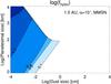 |
Fig. 13 Contours of the logarithm of the hydrodynamical factor log 10(fhydro) (see Eq. (105)) as a function of dust size (in cm) and planetesimal size (in km), at 1 AU in the MMSN. The physical density of dust and planetesimals is set to 1 and 3 g cm-3, respectively. The contours are for fhydro = 10-7, 10-6, 10-5, 10-0.5, 10-0.1. The transition from the hydrodynamic flow regime to the boundary regime (dark to light blue) takes place over a narrow range of dust sizes for planetesimals smaller than 100 km in radius. For larger planetesimal sizes, the transition between the hydrodynamic and settling regimes is discontinuous by construction. A proper modeling of this transition will require more work. |
4.5. Effect of turbulence
4.5.1. Amplitude of velocity fluctuations
Turbulence in the disk generates density and pressure fluctuations. For example, using direct numerical simulations in the shearing box approximation, Heinemann & Papaloizou (2009) find that spiral density waves excited by magneto-rotational instabilities (or another suitable mechanism) yield relative density fluctuations of about 15% of the mean values on length scale smaller than the pressure scale height. This would thus lead η, as calculated from Eq. (19)to vary significantly (even changing sign) over both space and time. However, this η is not a proper measure of the headwind that the particles feel because the gas associated with these density fluctuations is still moving azimuthally at a velocity close to the average gas velocity. Actually, the velocity dispersion of the particles is linked to that of the gas and may thus be written (Youdin & Lithwick 2007) 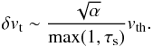 (106)In the simulations of Heinemann & Papaloizou (2009), δvt ~ 0.15vth (i.e., ~100 m s-1 at 1 AU) for α ~ 5 × 10⁻³ for the gas, which agrees well with Eq. (106). (We note that vth ~ 1 km s-1 at 1 AU in the MMSN.) Flock et al. (2013) also obtain similar values of α and slightly lower turbulent velocities in the range 10 − 100 m s-1 in the mid-plane, but an order of magnitude higher in the disk atmosphere heated both by stellar irradiation and MRI dissipation.
These velocity fluctuations obtained in MRI-active regions are of the same order of magnitude as the mean headwind felt by planetesimals ηvK ~ 50 m s-1. In these regions, turbulence can have an important role. In dead zones and generally in regions with much smaller values of α ~ 10-4 it can perhaps be neglected. We examine below two consequences of turbulence on the collision probability.
4.5.2. Consequence for the hydro mode
A first consequence of turbulence is that the flow around the planetesimal may not be adequately described as laminar as assumed in Sect. 4.4 and in simulations by Sekiya & Takeda (2003) and Sellentin et al. (2013). Recently, Mitra et al. (2013) simulated the accretion of dust by boulders (less than a km in size) in a turbulent flow and obtained results that strongly differ from the laminar case. In their simulations, dust (with sizes in the range 10 − 200 μm) is efficiently accreted by boulders of about 6 to 200 m. The speeds and accretion trajectories seem to differ from the laminar case. Unfortunately, in the absence of a description of the assumed turbulent flow and without a comparison to a purely laminar case, it is not possible to quantify the consequences of these results.
Qualitatively, we can tell that if the smallest scales of turbulence remain large compared to the size of the object considered, the laminar prescription defined by Eq. (105)should remain valid although modified to account for a mean flow velocity that differs from the laminar headwind velocity. This modification should lead to the accretion of grains of slightly smaller sizes without fundamentally affecting the picture. If, however, the turbulent cascade extends to scales as small as the size of the planetesimal and lower, it will modify the picture considerably and probably lead to a drastic reduction in the extent of the parameter regime affected by the hydro mode.
4.5.3. Turbulence factor and random walk
Beyond its effect on the hydrodynamical regime, turbulence also affects the collision probability. This can be estimated with the same approach as for the eccentric planetesimalin Sect. 4.1: the fluctuations of the velocity field along the planetesimal’s trajectory can be considered to average out to zero if they are smaller than the mean collision velocity, and to lead to an increased collision probability otherwise. We thus estimate the factor by which the final collision probability is increased over the geometrical limit due to turbulence by ![Mathematical equation: \begin{equation} f_{\rm t}=\sqrt{1+\left[{1+\taus^2\over \sqrt{1+4\taus^2}}{1\over \max (1,\taus)}{\sqrt{\alpha}\over \eta}{v_{\rm th}\over v_\rmK}\right]^2}\cdot \label{eq:ft} \end{equation}](/articles/aa/full_html/2014/12/aa23021-13/aa23021-13-eq424.png) (107)In the other regimes, we do not expect turbulence to lead to a significant increase of the collision probability and hence define the collision probability as
(107)In the other regimes, we do not expect turbulence to lead to a significant increase of the collision probability and hence define the collision probability as only if ft> max(fe,ffocus).
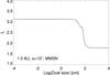 |
Fig. 14 Value of the turbulence factor ft (see Eq. (107)) as a function of dust size (in cm), at 1 AU in the MMSN for a turbulence viscosity parameter α = 10-2. We note that contrary to the other plots, the linear value of the factor is plotted instead of its log. |
As shown in Fig. 14, turbulence is expected to increase the mean collision probability in the geometrical limit only by a modest amount. When considering for example dust of 1 cm in size, the value of ft for α = 10-3 varies from a maximum of 1.9 at 0.1 AU to 1.03 at 100 AU. These values scale with  .
.
4.6. Additional effects relevant for massive embryos
The effects discussed previously apply to a wide range of planetesimal sizes. When considering planetary embryos with large masses, two effects should be included but are not taken into account in the present calculation.
4.6.1. Presence of an atmosphere
Big planetesimals (or protoplanets) with masses above 0.1 M⊕ (equivalently Rp~>5000 km for ) start to acquire an atmosphere. Inaba & Ikoma (2003) showed that the presence of a dense atmosphere increases the cross section of planetesimals and they derived expressions to quantify this effect. However, Ormel & Kobayashi (2012) showed that for small particles interacting in the settling regime the presence of an atmosphere does not yield an increase in the cross section. The presence of an atmosphere becomes important only when considering the three-body interactions between planetary embryos and very large dust particles, namely boulders or planetesimals.
4.6.2. Gap opening
Tidal interactions between massive protoplanets lead to the opening of gaps in circumstellar disks (e.g., Lin & Papaloizou 1985, 1993). These gaps suppress the flow of material between the outer disk and the inner disk and could be the reason behind the existence of the so-called transitional disks, i.e., disks with accretion onto the central star and a central cavity (e.g., Rice et al. 2006). Actually, gaps are opened more easily (i.e., by smaller-mass protoplanets) in the dust and/or planetesimal disk (e.g., Tanaka & Ida 1999; Paardekooper & Mellema 2004) than in the gas itself, implying a potentially high degree of filtering of material from the outer system. This effect cannot be accounted for in the expressions derived here. We merely note that the presence of massive protoplanets with masses larger than 10 M⊕ that can open up gaps in gas disks will certainly be accompanied by a drastic reduction of the metallicity of the gas flowing into the inner regions and accreted by the central star.
5. Collision probabilities
5.1. The 2D collision probability
We can thus calculate the final collision probability of a planetesimal of radius Rp, physical density , orbital semi-major distance r, eccentricity e, with a dust grain of size s and physical density  inside a disk as follows. We first need to define the characteristics of the gas disk at that orbital distance, in particular the disk temperature T, mid-plane density ρg, scale height hg, Keplerian velocity vK and η parameter (Sect. 2.1). We then need both the molecular and turbulent viscosities νg and ν, respectively, to calculate the drag forces, stopping time τs and τs,ν and thus the relative velocities Δvr and Δvθ between our planetesimal and dust particle (Sect. 2.4).
Armed with these quantities, we can easily calculate with Eq. (36)the 2D geometrical probability in the circular case  . For eccentric and/or inclined planetesimals, we estimate the probability increase by averaging the planetesimal’s cross section on its trajectory. The expression for the eccentricity-inclination factor fe,i is found in Eq. (78)(this factor is always larger than unity and is to be used instead of fe defined by Eq. (70)to account for a non-zero inclination). The inclusion of gravitational focusing is calculated analytically in three regimes, the Safronov, settling, and three-body regimes (see Sect. 4.3). The corresponding focusing factor ffocus is defined in Eq. (98). The planetesimal linear cross section b (equal to Rp in the geometrical limit) and encounter velocity Δvcol (equal to ηvKfe in the geometrical limit and assuming a small τs; see Eq. (69)) are defined in Eq. (99)(see Sect. 4.3). The value of ffocus is always larger than unity.
We account for a decrease in the collision probability due to the hydrodynamical flow around the planetesimal through the factor fhydro, defined in Eq. (105). This factor is always smaller than unity, and in fact becomes very small when the dust particle stopping time becomes smaller than the planetesimal crossing time, i.e., when the friction parameter τf defined by Eq. (100)becomes smaller than unity. We also account for the velocity dispersion of dust particles due to turbulent fluctuations in the gas disk through the factor ft defined by Eq. (107). This factor is larger than unity, i.e., turbulence always increases the probability of a collision.
The final 2D collision probability is written  (108)where fhydro ≤ 1, whereas other factors are always equal to or larger than unity. We note that values of
  above unity correspond to multiple collisions.
Figure 15 shows the 2D probabilities that result from including all these processes at 1AU in the MMSN case (see Appendix A) for a variety of combinations of dust and planetesimal sizes. At this location, particles with s ~ 1 m have τs ~ 1 and thus are the ones that have the largest relative velocities and smallest accretion probability. The probability decrease due to the hydrodynamic flow around planetesimals (for τf~<1) is evident in the upper left hand corner of the figure, but it is limited to relatively large planetesimals (above 1km for micron-sized dust): this is because the interaction time for the gas around small planetesimals is too short compared to the stopping time of even small dust particles.
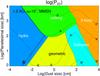 |
Fig. 15 2D collision probability |

5.2. The 3D collision probability
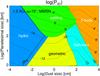 |
Fig. 16 Collision probability |

The final collision probability accounting for 3D effects,  , is obtained from and Eq. (108)and Eq. (43). Figure 16 shows the values of at 1 AU as a function of dust and planetesimal sizes. Except when it reaches very large sizes for the planetesimals (i.e., in the planet-regime), the probability is several orders of magnitude smaller than because the dust layer is much thicker than the planetesimal cross section. This reduction is more pronounced for small grains, because they are spread over a thicker disk and for small planetesimals because of their smaller cross section. Otherwise, we can see that planetesimals with sizes below ~100 km have collision probabilities that are close to the geometrical ones (see Eq. (44)) and scale with the square of their size, except for those with small dust grains which take place in the hydrodynamical regime and become much less likely. For larger planetesimals, collisions can take place in the settling regime or, for large grains, in the three-body regime. Because of a significant focusing factor, these collisions become more dependent on planetesimal size (and mass).
Importantly, Fig. 16 shows that for a wide variety of planetesimals dust sizes, the collision probability remains significantly smaller than unity. This means that embryos less massive than an Earth mass can capture only a small fraction of the grains flowing through the disk. As shown in Appendix C, the situation is more favorable for smaller values of α since  , but this is not sufficient for a large fraction of the dust sizes to be considered.
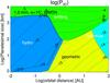 |
Fig. 17 Same as Fig. 16, but with the collision probability |
Figure 17 shows the same probability , but for 1 mm dust grains as a function of orbital distance. Most collisions in this figure fall into a hydro, geometric, or settling regime. The hydro regime is widespread and extends to up to ~1 AU for a variety of planetesimal sizes, indicating that grains smaller than millimeter size must be either captured at larger orbital distances by small planetesimals (3 km in radius), or through same size collisions. In the geometrical regime, depends strongly on planetesimal size and inversely on orbital distance. As demonstrated in Appendix C, in that regime  , because the geometrical probability scales as 1/(hgr) and hg ∝ r5/4 in the MMSN. On the other hand, in the settling regime, is even more strongly dependent on planetesimal size (it becomes dependent on its mass), but very weakly on orbital distance. Thus, as shown in Appendix C for the settling/Bondi regime,
  for small dust particles, and
  for medium-sized dust particles. The dependence of τs and particle size on orbital distance implies that the probability can increase with orbital distance, as is the case in some regions of Fig. 17.
6. Are planetesimals efficient dust filters?
6.1. Filtering efficiency at 1 AU
We now revisit the filtering efficiency as defined in Sect. 3.4 for the geometrical circular limit, but this time applying the full treatment including eccentricities, gravitational focusing, hydrodynamical effects and turbulence. We employ the parameter xfilter as defined by Eq. (58)and a value of the surface density of planetesimals Σp(r) equal to the MMSN disk of solids. A value of xfilter,MMSN(s) close to unity or larger thus implies an efficient filtering of dust grains of size s by a mature disk of planetesimals. A lower value implies an inefficient filtering of the dust particles by this disk.
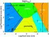 |
Fig. 18 Contours of the filtering efficiency by a MMSN planetesimal disk at 1 AU for α = 10-2, assuming monodisperse size distributions for planetesimals and dust grains. The contour indicating perfect filtering efficiency for log 10xfilter = 0 is shown in bold. |
Figure 18 shows the values of xfilter,MMSN(s) at 1 AU as a function of dust and planetesimal size (both are assumed to have a single size distribution). Dust of millimeter size or less is generally transported by the flow around the planetesimals and can only be accreted by small planetesimals in the geometrical regime or by large ones in the settling regime. Its filtering in the inner solar system appears to be inefficient. In the geometrical limit, filtering is relatively efficient for small planetesimals but decreases inversely with the planetesimal size until it reaches the settling regime. There, for planetesimals in the range 100 − 1000 km and beyond, a higher efficiency results from the Bondi-accretion regime. For large dust particles with a large stopping time, the slow radial drift has the consequence that dust and planetesimals have more time to interact gravitationally resulting in a more efficient filtering. However, only particles of 10 meters or more appear to be efficiently captured by planetesimals of any size. (This does not necessarily imply high accretion rates, however, because these relations implicitly assume an infinite time for the interaction.)
6.2. Filtering efficiency vs. orbital distance
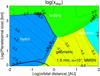 |
Fig. 19 Contours of the filtering efficiency by a MMSN planetesimal disk for 1 mm dust for α = 10-2, assuming a monodisperse size distribution for planetesimals. The contour indicating perfect filtering efficiency for log 10xfilter = 0 is shown in bold. |
Figure 19 shows the filtering efficiency for millimeter particles as a function of orbital distance. Strikingly, these particles are very inefficiently filtered inside of 1 AU, or only by either very small planetesimals or relatively large planetary embryos. The orbital dependence of filtering depends strongly on the collision regime: for small planetesimals, for which collisions with mm-sized grains take place in the geometrical regime, filtering is highly dependent on orbital distance. As shown in Appendix C, xfilter ∝ r− 7/4, which would favor the growth of the very first planetesimals very close to the central star. On the other hand, Fig. 19 shows that in the settling regime, filtering is more weakly dependent on orbital distance. Appendix C shows that xfilter ∝ r− 1/4 in the settling/Bondi regime and xfilter ∝ r1/4 in the settling/Hill regime. Farther from the central star, planetary embryos can perturb the motion of dust particles to much larger distances.
Thus, while small planetesimals can filter dust only if they are close to the central star, the filtering properties of planetary embryos are relatively independent of orbital distance. This could help to understand why the inner solar system appears to have a gradation of composition whereas the outer solar system seems more uniform.
6.3. Filtering as a function of the mass of gas in the disk
Figure 20 shows how the filtering efficiency varies with dust size and as a function of the factor, i.e., as the gas disk evolves and progressively becomes less dense, for a turbulent viscosity set by α = 10-2. We have assumed in all cases that a collision cascade maintains a population of planetesimals with radii between 1 km and 1000 km with a mass exponent q = 3.5 and a surface density equal to the MMSN in solids.
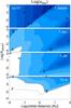 |
Fig. 20 Filtering efficiency of a swarm of planetesimals with radii between 1 km and 1000 km as a function of orbital distance and |
Clearly, filtering is most ineffective for small, micron-sized particles, mostly because they are in a hydrodynamical regime and thus avoid planetesimals and/or because turbulence lifts them up. This occurs at all orbital distances and for all values of . Larger particles are progressively easier for the planetesimal swarm to collect, with a filtering that is more efficient in the inner regions than in the outer ones. Millimeter-sized particles begin to be more efficiently collected at orbital distances shorter than 0.1 AU and only for χMMSN< 10-2, i.e., when the gas density has become small enough to reduce the inward drift of dust significantly. Centimeter-sized particles may also be collected more efficiently regardless of , but only inside 0.1 AU. Particles of 10 meters or more are efficiently collected as soon as the gas density becomes of the same order as or lower than that of the MMSN. This is a direct consequence of the slower gas drag and hence slower inward drift of these particles at later ages.
Apart from small dust particles in the hydrodynamical regime and large boulders, the filtering properties of planetesimals remain remarkably stable and independent of the evolution of the gas disk inside about 3 AU. It is interesting to see that the filtering efficiency remains relatively large (between 0.1 and 0.01) in a zone between 0.1 AU and 1 AU, but that it drops and becomes dependent on the evolution of the disk beyond about 3 AU.
Even when xfilter ≈ 1, filtering can be considered to be moderately efficient because this corresponds to a mass in planetesimals equals to that of the present solar system. For a smaller mass, as would presumably occur in a young planetesimal disk, the filtering efficiency would be reduced by a ratio equal to that between the mass of the planetesimal disk to the MMSN. Figure 20 thus shows that in order to efficiently capture small (centimeter-sized or less) dust particles, they have to be first assembled into larger planetesimals of at least 10 meters or more by a different mechanism such as orderly growth (by collision of grains of the same-size) or a streaming instability. Alternatively, filtering could be done more efficiently by planetesimals smaller than 1 km which will also drift and have thus not been considered in this study.
6.4. Filtering by an extended belt of planetesimals
We now consider the filtering of dust by a belt of planetesimals assumed to extend between 0.1 AU and 35 AU. We calculate Xfilter as defined by Eq. (56), but assuming a monodisperse size distribution of planetesimals. We neglect any variations of dust size (e.g., due to growth or vaporization at the ice line) in the integration over orbital distances. A value of Xfilter larger than unity indicates an efficient filtering of dust by the planetesimal belt. It also implies that the star accretes gas that is poor in dust of that size.
Figure 21 shows that for our fiducial value of α = 10-2 the filtering by a belt of planetesimals is efficient only for large dust sizes beyond about 10 meters. Two islands of higher filtering are for planet embryos (Rp~>1000 km) and pebbles of centimeter to meter size, or when planetesimals are very small (Rp~<10 km) for dust larger than millimeter size. These correspond to collisions in the settling and geometric regimes, respectively.
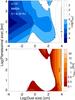 |
Fig. 21 Filtering efficiency of dust of 1 micron to 100 meters by a MMSN planetesimal belt with planetesimals of 1 to 10 000 km in radius extending from 0.1 to 35 AU for a turbulent parameter α = 10-2 and assuming monodisperse size distributions for planetesimals and dust grains. Top panel: contours of the disk-integrated filtering factor Xfilter. Bottom panel: orbital distance at which Xfilter(r) = 1 for dust particles drifting in from beyond 35 AU. (The integration thus starts from 35 AU and goes inwards.) |
Even in these islands, dust is able to penetrate deep inside the planetesimal belt, most of it reaching orbital distances between 0.1 AU to 1 AU. The clear gradient in the abundance of ices measured in the asteroid belt and its scarcity in asteroids that are closer than 2 AU to the Sun implies that either the gas disk was much less turbulent or another physical mechanism led to the present composition of the solar system.
6.5. Filtering in a weakly turbulent disk
We now turn to the case of a weakly turbulent disk (or equivalently, a disk with an extended dead-zone) by considering the case of a turbulent parameter α = 10-4. This case is more favorable because dust settles closer to the mid-plane and the mean gas flow is also slower. Appendix C demonstrates that for most grain sizes, xfilter ∝ α− 1/2. Appendix D provides the same figures as in the previous sections, but for the weak-turbulence case instead of the fiducial α = 10-2. In all cases, filtering is found to be much more efficient.
This is exemplified by Fig. 22 which shows the integrated filtering coefficient as a function of planetesimal and dust sizes for α = 10-4. The two islands of efficient filtering previously observed in Fig. 21 are now much wider and more pronounced. Large embryos (Rp~>1000 km) can now efficiently filter dust between millimeter and meter size in the settling regime. This is directly linked to the efficient accretion of pebbles by protoplanetary cores discussed by Ormel & Klahr (2010) and Lambrechts & Johansen (2012). (It should be noted that this requires a small value of the planetesimal scale height hp, as discussed in Appendix E.) Small planetesimals are able to efficiently filter small dust in the geometric regime and millimeter-sized dust particles can now be captured beyond 1 AU, in better agreement with the meteoritic record.
It is thus possible to imagine that the relative lack of water in the inner solar system may have been due to filtering of ice grains by planetesimals and/or planet embryos beyond 2 to 3 AU in a weakly turbulent disk and/or by its inefficient capture around 1 AU. Conversely, the presence of abundant chondrules of micron to millimeter-size in meteorites may be due both to their inefficient filtering by planetary embryos and their more efficient capture by small size planetesimals. At this point, without a proper model to predict the distribution of sizes of planetesimals and its evolution, these are only conjectures. However, we may affirm that the complex dependency of filtering with planetesimal and dust size must have played a crucial role in shaping our solar system.
6.6. Compact vs. porous grains and planetesimals
We have so far assumed a canonical 1 g cm-3 physical density both for planetesimals and grains. We know that small particles, from dust grains to asteroids are porous and may therefore be characterized by small densities (e.g., Consolmagno & Britt 1998; Dominik & Tielens 1997; Kataoka et al. 2013). On the other hand, large planetesimals and protoplanets are affected by compression effects and will generally have higher densities. Interestingly both tend to lead to a higher filtering efficiency than for our baseline density. For small planetesimals in the geometrical limit, the filtering efficiency derived by Eq. (60)is ∝ because, for a given total mass of planetesimals (that defined by the MMSN) and a given size, the number of planetesimals is proportional to the inverse of their physical density. Porous planetesimals will therefore be more efficient filters in the geometric regime. In the settling regime, the filtering efficiency directly depends on the mass of the planetesimal, not on its density.
6.7. Filtering by protoplanets
Even though our parameter range extended to radii of 104 km (corresponding to a mass of 0.7 M⊕ for ), our study has focused on smaller planetesimals. For protoplanets, two effects that have not been taken into account become gradually more important.
First, protoplanets with masses over ~0.1 M⊕ (corresponding to radii of about 5000 km for ) begin building a hydrogen-helium atmosphere which progressively enhances their cross section (Inaba & Ikoma 2003; Tanigawa & Ohtsuki 2010). When modeling this effect with the approach of Ormel & Kobayashi (2012), we find that the effect is significant at the high end of the radius range considered here, but without affecting our conclusions: the filtering efficiency remains low even for these Earth-mass protoplanets when in the settling regime, and extremely low in the hydrodynamical regime.
For even larger masses (outside the range of this study), we can expect atmospheric capture to continue to increase, but it is progressively balanced by the fact that at masses ~30 M⊕ (~0.1 MJ) protoplanets start opening gaps in the dust disk, thereby strongly suppressing or even halting their capture (Paardekooper & Mellema 2004; Morbidelli & Nesvorny 2012). The consequence is that the growth of giant planet cores should lead to a parking of dust outside of the orbit of the core farthest from the central star. This effect is most significant for particles with τs ~ 1. These particles would neither be captured efficiently nor be accreted by the central star, which is a form of filtering that differs from the one discussed thus far. Presumably, these should eventually lead to the formation of a belt of planetesimals such as the Edgeworth-Kuiper belt in the solar system.
6.8. Consequence for planet growth
As discussed previously, the island of higher filtering efficiency in the settling regime (for Rp~>1000 km) seen in Figs. 22 (see also Fig. D.1) is directly linked to the efficient accretion of pebbles by protoplanetary cores found by Lambrechts & Johansen (2012). The increase in the filtering efficiency with planetesimal radius in the settling regime results from the very fast increase in the Bondi radius and hence planetesimal cross section (for dust of the right size), which more than compensates for the fewer objects for a given mass of planetesimals. This effect begins for sizes around 100 km when the Bondi surface becomes larger than the planetesimal itself, and continues to the point where the Bondi and Hill radii are equal (around 1200 km for planetesimals at 1 AU; see Appendix A), and beyond.
Although the filtering factors xfilter and Xfilter approach or exceed 1, we stress that this occurs in a relatively small region of the parameter space in terms of planetesimal and dust sizes. Given that planetesimals must have had a wide range of sizes, it is not clear that filtering could be complete, even for weakly turbulent disks. We notice that the collision probabilities obtained for large embryos are generally significantly smaller than unity (see Fig. 16 and Appendix C). This seems to imply that the rapid growth of giant planets cores by pebble accretion (Lambrechts & Johansen 2012) is mostly driven by the fast inward flow of pebbles and requires a very large mass of solids in the disk, several times larger than the embryos to be created (~10 M⊕ or more for giant planet cores). However, a recent work by Lambrechts & Johansen (2014) shows that pebbles could grow to the right sizes (cm to mm) to be effectively captured by large embryos beyond an Earth mass. We note that the high filtering efficiency bands seen in the settling regime in Figs. 21 and 22 for s ~ 1 − 100 cm and Rp~>1000 km extend to high Rp values (large embryo masses) beyond the limit of the graphs. Thus, assuming that large embryos (Mars to Earth mass) may be formed rapidly by another mechanism, this opens the possibility of an efficient conversion of dust to planets, as obtained by Lambrechts & Johansen. Also, because of the ability of small planetesimals to filter dust grains (and pebbles), a convoluted environment of interacting planetesimals, fragments, and pebbles, like that studied by Chambers (2014), could, under the right conditions, limit the loss of solids onto the central star.
More work is required, however, especially since collisions do not necessarily result in accretion (e.g., Sekiya & Takeda 2003; Blum & Wurm 2008; Johansen et al. 2014) as we have implicitly assumed for this discussion.
7. Conclusions
Abundant micron- to centimeter-sized dust is detected in protoplanetary disks in spite of theoretical predictions of a fast inward drift of these particles due to gas drag. We have studied whether this dust may be efficiently filtered by planetesimals and thus contribute to their growth, the formation of planets and the final composition of stars with planets.
In most cases, the planetesimal disk can be considered vertically thinner than the dust subdisk which is itself thinner than the gas disk. Dust particles drift inward as a result of gas drag but also because of the advection of gas (Eq. (23a)). For all of these grains, turbulence and epicyclic motions lead to frequent crossings of the mid-plane. We showed that the filtering length, i.e., the distance over which we can expect most particles to have crossed the mid-plane during their inward drift, is on the order of ηr ~ 10-3r where r is the orbital distance (Eq. (30)). This low value implies that particles may be filtered by the planetesimals even if they are initially high up in the disk.
We thus derived the collision probability between a non-drifting planetesimal and a drifting dust particle in the geometrical limit (Eq. (45)). This probability depends on the ratio of the surface of the planetesimal  to the vertical surface of the disk hgr multiplied by a factor that depends on the values of α and τs which control both the characteristic vertical extent of the dust subdisk and the inward drift speed of the particles. Assuming a size distribution of planetesimals set by a collisional cascade, we derived the filtering efficiency (Eq. (56)), i.e., the efficiency at which particles would be trapped by the planetesimal swarm. Small planetesimals dominate this regime because of their large collective surface area. The global filtering efficiency for an MMSN disk of 1 km radius planetesimals at 1 AU in a quiescent disk with α = 10-4 was found to be close to unity for millimeter-sized grains, and between 0.1 and 10 for all grain sizes considered. It is inversely proportional to the planetesimal density and radius. It also scales with α− 1/2 for all except the smallest grain sizes, implying a better filtering in quiescent parts of the disk (dead zones). Last but not least, it has a strong dependence on the orbital distance, r− 7/4, implying that filtering in the geometric regime is more efficient close to the central star (see Eq. (61)and Fig. 5).
We then considered additional mechanisms. We showed that given the small expected values of the eccentricities and inclinations of the planetesimals in these young gas disks, the increase of the collision probabilities caused by these non-circular orbits is expected to be small (Fig. 7). Gravitational focusing was found to be significant for planetesimals larger than about 100 km and/or dust (or rather boulders) beyond meter size (Fig. 10). However, small grains with a stopping time shorter than the planetesimal crossing time (Eq. (100)) are carried by the hydrodynamical flow around the planetesimals, yielding a strongly reduced collision probability (Eq. (105)and Fig. 13). Turbulence in the disk was estimated to have a limited effect (Eq. (107)and Fig. 14), but confirming this result would require direct simulations.
On the basis of these calculations, we examined whether planetesimals are efficient filters of dust in protoplanetary disks. Large “dust” particles over 10 meters drift inward so slowly that they can be captured efficiently by planetesimals of any size (Fig. 18). Small dust particles (below millimeter size) generally have a low collision probability with planetesimals because of the hydrodynamical effect, at least at orbital distances of an AU or less. In between, millimeter dust to pebbles of tens of centimeters are captured in the geometrical regime by planetesimals smaller than 100 km, but in the settling regime by larger planetesimals (Figs. 18 and 19). The capture law for the latter is very different than in the geometrical regime: it is independent of the planetesimal density and is proportional to r− 1/4 in the settling/Bondi regime and r1/4 in the settling/Hill regime (Eq. (C.16)). This implies that filtering in the settling regime is more uniform than in the geometrical regime. We can therefore expect that early, small planetesimals grew rapidly by capturing dust in the geometrical regime, creating an inside-out planetesimal formation front. Larger planetesimals would have been able to capture dust out to larger orbital distances.
Locally, the filtering efficiencies defined by xfilter are generally low: they reach unity only at orbital distances below about 0.05 AU and for grains of millimeter size and larger for a turbulence parameter α = 10-2. At 1 AU, grains from millimeter to meter size are captured with only a ~1% efficiency for an MMSN disk of planetesimals for α = 10-2, and ~10% for α = 10-4 (Figs. 18 to D.2). Less turbulence increases the filtering efficiency, but not enough for an efficient capture of the solids in the disk. Separately, the fact that the gas disk progressively becomes less massive does not change the filtering efficiencies, except for very small grains (which are more easily accreted as time goes by), and beyond a few AUs (where filtering becomes less efficient before increasing again for very tenuous disks) (Figs. 20 and D.3). Accounting for the fact that small planetesimals may be more porous and that large planetesimals should be more dense than our canonical 1 g cm-3 density would help to increase the filtering efficiency close to 100 % at around 1 AU from the central star.
Once a belt of planetesimals forms and grows over a large range of orbital distances, it may be able to filter the incoming dust more effectively, especially in weakly turbulent disks. Values of the integrated filtering efficiency Xfilter defined by Eq. (56)(Figs. 21 and 22) show the existence of essentially three regimes: planetesimals smaller than about 10 km are very efficient at filtering dust, but because of the strong radial dependency, this must occur close to the central star. Planetesimals between 10 km and 1000 km in size are inefficient at filtering because of their smaller surface-to-mass ratio and absence of gravitational focusing. Planet embryos larger than 1000 km are more efficient at filtering dust, and contrary to small-size planetesimals, this occurs over a wide range of orbital distances.
Accounting for the size distribution of individual particles assembled in meteorites is a complex task that would require a full model accounting for the evolution of the size distribution of planetesimals and dust particles everywhere in an evolving protoplanetary disk. We simply mention that the absence of grains larger than about ~1 cm in meteorites appears to be consistent with our finding that these would be captured preferentially in large embryos. Conversely, two features can explain the size distribution of chondrules in meteorites (see, in a different context Cuzzi et al. 2001): grains smaller than centimeter-size are captured preferentially in small-planetesimals, and moreover, grains of smaller sizes are increasingly more difficult to capture, as a consequence of the hydrodynamical flow around these planetesimals.
Obviously, the question of whether dust can be efficiently filtered by planetesimals is a complex one that touches on many physical problems ranging from the unclear structure of circumstellar disks, angular momentum transport processes, efficiency of turbulence, growth processes, etc. We hope that our study can lay the ground for further studies. For example, direct simulations of planetesimals and dust at the interface between the hydrodynamical and settling regimes would be needed. The influence of turbulence has been approximated here and appears to be limited, but this would need to be confirmed on the basis of realistic simulations. We have also used mean approaches, but rare statistical events could matter and change the picture. Last but not least, we implicitly assumed that collisions result in sticking. In reality, this will strongly depend on the velocities involved, leading to a wide range of possibilities. Understanding the evolution of young stars, their composition, and that of planetary systems requires these dedicated studies.
Online material
Appendix A: The minimum mass solar nebula scaling
We provide in Table A.1 the main quantities that are used in the article and present their scaling in the so-called minimum mass solar nebula formalism (Hayashi 1981; Nakagawa et al. 1986).
Expressions for the minimum mass nebula scaling used in this article.
Appendix B: Geometric collision probability with shear
We derive the expression for the geometric collision probability and show that it is identical to that derived by Ormel & Klahr (2010). From Eqs. (23a) and (23b) and accounting for both the (assumed inward) radial velocity of the gas due turbulent viscosity vν and the shear in the disk, 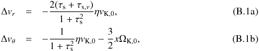 where, following Ormel & Klahr (2010), we have used an expansion around the location of the planetesimal (ΩK,0 ≡ ΩK(x = 0)), and x is the radial distance from the planetesimal at which the collision with the dust particle takes place. For simplicity, we assume that on average x = Rp/ 2. This yields the impact rate in the geometrical limit as:
 ![Mathematical equation: \appendix \setcounter{section}{2} \begin{equation} {\cal R}_{\rm 2D,geo,circ}=2R_\rmp\eta v_\rmK {2(\taus+\tausnu)\over 1+\taus^2} \sqrt{1+\left[{4\eta +3(R_\rmp/ r)(1+\tau_\rms^2)\over 8\eta(\taus+\tausnu)}\right]^2}, \label{eq:A_Rgeocirc} \end{equation}](/articles/aa/full_html/2014/12/aa23021-13/aa23021-13-eq551.png) (B.2)where we have dropped the 0 labels. When vν = 0, this expression is equivalent to Eq. (22) of Ormel & Klahr (2010) who derive this impact rate by an analysis of the trajectory of dust particles. In most cases, we will consider ητs ≪ Rp/r so that shear may be neglected and
(B.2)where we have dropped the 0 labels. When vν = 0, this expression is equivalent to Eq. (22) of Ormel & Klahr (2010) who derive this impact rate by an analysis of the trajectory of dust particles. In most cases, we will consider ητs ≪ Rp/r so that shear may be neglected and  : the collision rate is the product of the cross section 2Rp and the encounter velocity
  .
.
The 2D probability that a planetesimal will accrete a given dust grain is then given by Eq. (35): ![Mathematical equation: \appendix \setcounter{section}{2} \begin{equation} {\cal P}_{\rm 2D,geo,circ}={R_\rmp\over \pi r}\sqrt{1+\left[{4\eta +3(R_\rmp/ r)(1+\tau_\rms^2)\over 8\eta(\taus+\tausnu)}\right]^2}\cdot \label{eq:A_P2Dcirc} \end{equation}](/articles/aa/full_html/2014/12/aa23021-13/aa23021-13-eq556.png) (B.3)This equation may be approximated in the different regimes (from small to large particles):
(B.3)This equation may be approximated in the different regimes (from small to large particles): ![Mathematical equation: \appendix \setcounter{section}{2} \begin{equation} {\cal P}_{\rm 2D,geo,circ}\approx {R_\rmp\over \pi r}\max\left[{1\over 2(\taus+\tausnu)},1,{3\over 8}{R_\rmp\over r}{\taus\over \eta}\right]\cdot \label{eq:A_P2Dcirc_approx} \end{equation}](/articles/aa/full_html/2014/12/aa23021-13/aa23021-13-eq557.png) (B.4)The lowest capture probability Rp/πr corresponds to dust particles with τs ~ 1 which drift in with a speed that is comparable to the headwind felt by the planetesimal. One can expect that these particles will be the most difficult to filter. For smaller τs values, the slower drift leads to a higher probability, limited by the gas drift. For large τs values, the drift rate also decreases and the effect of the Keplerian shear across the planetesimal becomes dominant. The capture probability then becomes a very steep function of the planetesimal size (∝
(B.4)The lowest capture probability Rp/πr corresponds to dust particles with τs ~ 1 which drift in with a speed that is comparable to the headwind felt by the planetesimal. One can expect that these particles will be the most difficult to filter. For smaller τs values, the slower drift leads to a higher probability, limited by the gas drift. For large τs values, the drift rate also decreases and the effect of the Keplerian shear across the planetesimal becomes dominant. The capture probability then becomes a very steep function of the planetesimal size (∝ in the Epstein regime and ∝
 in the Stokes regime). However, shear becomes important only for very large planetesimals (
 for the MMSN). It only concerns cases for which the collisions take place in the settling or three-body regimes. Shear can thus be neglected for the geometrical regime.
Appendix C: Analytical estimates for small grains (geometric, hydro, and settling regimes)
We provide here analytical estimates for the collision probabilities and filtering efficiencies for the geometric and settling regimes. In order to provide tractable relations, we make the following simplifications:
-
We study only small particles such that τs< 1, corresponding generally to s~<1 m.
-
Given the above assumption, we use Δv = ηvK for the dust-planetesimal encounter velocity.
-
We approximate χα,τs defined by Eq. (46)as follows:
 (C.1)We thus separate small particles with τs ≤ τs,ν ~ 0.32α which have not settled from larger particles for which hd(τs) <hg.
 -
We consider cases for which the planetesimal capture radius is smaller than the dust disk scale height and thus Eq. (43)can be simplified as:
 (C.2)
(C.2) -
We do not consider the Safronov and three-body regimes.
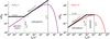 |
Fig. C.1 Value of the effective capture radius bset in units of the Bondi radius rB from Eq. (90)(colored curves) together with the approximation used in Eq. (C.3)(thick black lines). Left panel: solution when the Bondi radius is smaller than the Hill radius. Right panel: solution when the Bondi radius is larger than the Hill radius (specifically, the solution of Eq. (90)is shown for RB/RH = 10). |
Given a known encounter velocity, the calculation of the collision probability only requires that of the planetesimal effective capture radius. We know that it is extremely small in the hydro regime and equal to Rp in the geometric regime. In the settling regime, it is given by Eq. (90). As shown in Fig. 9, the settling regime may be subdivided into a Bondi regime in which the capture radius is proportional to  , and a Hill regime in which the capture radius is approximatively independent of τs and equal to the Hill radius. We thus approximate the effective capture radius of planetesimals/embryos in the different regimes as
 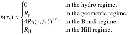 (C.3)and is defined by Eq. (88). The different regimes are defined by the following relations:
  (C.4)The dimensionless stopping times for the different regimes are defined by Eq. (88)for , Eq. (100)and τf = 1 for
  ,
,  for
for  , and
, and  for τHill. These and their MMSN approximations are thus respectively:
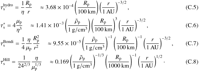 It can be seen that the value of is proportional to μp and reaches for the Hill-dominated settling regime (Rp ~ 1000 km). Importantly,
 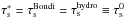 for
for  , with
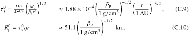
Appendix C.1: Collision probabilities
Using Eqs. (C.2), (31), (35), (80), (81), and (88), the collision probabilities for the three regimes defined in Eq. (C.3)can be written 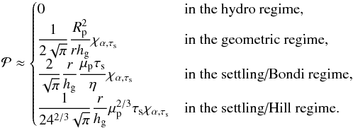 (C.11)When using the approximation from Eq. (C.1)and the MMSN scalings from Appendix A, this yields for small particles such that τs< 0.09α:
 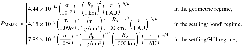 (C.12)and for medium-sized particles such that
 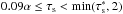 :
:  (C.13)We note that in these expressions, the scaling of the particle size (stopping time) was adjusted to be centered on the maximum collision probability in each regime.
 |
Fig. C.2 Value of the collision probability |


Figure C.2 shows that the simplified solutions are good approximations of the full solutions, except for large grains with τs~>2 and at the interface between the settling and geometric regimes (along the line). In the settling regime, the maximum collision probability is obtained for dust such that  , i.e., with a stopping time equal to the Hill sphere crossing time. For a low value of the turbulence parameter α = 10-4, a 1 M⊕ embryo (corresponding to Rp = 11250 km for a density) would have
  /
/ for particles such that
 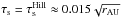 , i.e., for centimeter-sized pebbles between 1 AU and 10 AU.
Appendix C.2: Filtering efficiency
The filtering efficiency as defined by Eq. (58)writes for the regimes considered: 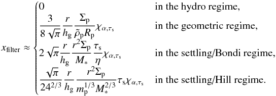 (C.14)The MMSN scaling then yields, for small particles such that τs< 0.09α:
 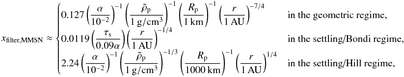 (C.15)and for medium-sized particles such that :
 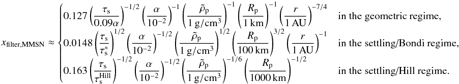 (C.16)
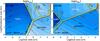 |
Fig. C.3 Value of the filtering efficiency log xfilter obtained by the full theory (black contours) and by the simplified one (red contours), for the MMSN and α = 10-4. The two panels are for two orbital distances: 0.1 AU (left) and 5 AU (right). (See Fig. C.2 for a full description.) |
Figure C.3 compares the values of xfilter obtained with the full theory and the simplified one, again showing good agreement except for large grains beyond meter size and near the line. For increasing planetesimal sizes, the maximum filtering efficiency is obtained along  , then
  and finally .
Appendix D: Results for a disk with α = 10-4
Given the inefficient filtering obtained in the high turbulence (α = 10-2) case, we now consider the weak turbulence case (α = 10-4). This is more favorable because dust settles closer to the mid-plane and the mean gas flow is also slower.
Figures D.1 and D.2 show the resulting filtering efficiency, both at 1 AU and for 1 mm dust, as a function of orbital distance. At 1 AU, efficient filtering is achieved for a wider range of dust and planetesimal sizes, basically for dust of 10 μm to 1 cm and planetesimals of less than a few kilometers in radius. A small island with xfilter~>1 also appears in the settling regime, for meter-sized dust and planetesimals of ~1000 km in radius. Compared to Figs. 18 and 19 in the α = 10-2 case, there is about an order of magnitude increase in the filtering efficiency.
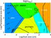 |
Fig. D.1 Contours of the filtering efficiency by a MMSN planetesimal disk at 1 AU for α = 10-4, assuming monodisperse size distributions for planetesimals and dust grains. The contour indicating perfect filtering efficiency for log 10xfilter = 0 is shown in bold. |
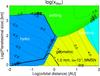 |
Fig. D.2 Contours of the filtering efficiency by a MMSN planetesimal disk for 1 mm dust for α = 10-4, assuming a monodisperse size distribution for planetesimals. The contour indicating perfect filtering efficiency for log 10xfilter = 0 is shown in bold. |
Figure D.3, shows how a lower value of the turbulence parameter α = 10-4 affects filtering by a distribution of planetesimals between 1 km and 1000 km. Compared to Fig. 20 for α = 10-2, filtering is found to be more efficient of course. For example, dust of 1 mm in size can now be efficiently captured in an MMSN disk inside about 0.03 AU while a value of xfilter = 1 is never reached for the high turbulence case until the gas disk has shrunk to about 1% of the MMSN value. Similarly, 1 cm grains can be captured with an efficiency close to unity inside of 0.1 AU compared to about 0.05 AU for the α = 10-2 case. In the 0.1−1 AU range, a wide range of small grains may be captured with an efficiency between 1 and 0.1. The dependence as a function of remains relatively weak, as in the strong turbulence case.
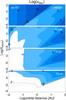 |
Fig. D.3 Filtering efficiency of a swarm of planetesimals with radii between 1 km and 1000 km as a function of orbital distance and mass of the gas disk for α = 10-4. (See Fig. 20 for details.) |
Appendix E: Dependence on the planetesimal scale height
All the results presented so far have assumed a rather low value of the planetesimal scale height hp = 0.01hg. This favors the filtering of particles able to settle to the mid-plane in a thin plane. In Fig. E.1 we show how the integrated filtering efficiency Xfilter depends on the value of hp. We select a low value of the turbulence parameter α = 10-4 because this is where the differences are most important. With an infinitely thin planetesimal disk (hp = 0, left panels), we obtain results that are very similar to our fiducial case (hp/hg = 0.01) shown in Fig. 22.
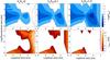 |
Fig. E.1 Filtering efficiency of dust from 1 micron to 100 meters by a MMSN planetesimal belt with planetesimals of 1 − 10,000 km in radius extending from 0.1 to 35 AU for a turbulent parameter α = 10-4 and various ratios of the planetesimal to gas scale height, from an infinitely thin planetesimal disk with hp/hg = 0 (left panels), hp/hg = 0.1 (middle panels), and hp/hg = 1.0 (right panels). As in Figs. 21 and 22, the top panels show the contours of the disk-integrated filtering factor Xfilter while the bottom panels show the orbital distance at which Xfilter(r) = 1 for dust particles drifting in from beyond 35 AU. |
When we increase the planetesimal scale height, the filtering of large particles becomes less efficient, as shown by the middle and right panels of Fig. E.1. Specifically, compared to the case when hp = 0, changes occur for particles larger than about 1 cm when we consider hp/hg = 0.1 and for particles larger than about 0.1 cm when we consider hp/hg = 1.0.
We first consider the limit for which Eq. (43)becomes independent of hp and the problem may be considered 2D. This occurs when the cross section of the embryos becomes so large that b> (2/ . By writing β ≡ RH/b, one may show that this occurs when
 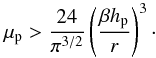 (E.1)For the MMSN disk at 1 AU, this is equivalent to
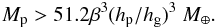 For large embryos we expect β~>1 with a significant dependence on τs (see Appendix C). In the regime that we considered in this work Eq. (E.1)is not satisfied, but it would be for embryos larger than a few Earth masses which may then accrete more efficiently.
The decrease of the filtering efficiency with increasing hp value seen in Fig. E.1 is hence a direct consequence of the fact that when Eq. (E.1)is not satisfied, the 3D collision probability given by Eq. (43)depends on the maximum of hd and hp. The probability thus becomes dependent on hp when hp>hd, that is when 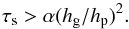 (E.2)For α = 10-4, this implies that we expect lower collision probability and filtering efficiency when compared to the hp = 0 case when τs = 10-2 for hp/hg = 0.1 and τs = 10-4 for hp/hg = 1. According to Fig. 3 (around 1 AU), this corresponds to s ≈ 1 cm and 1 mm, in good agreement with the results of Fig. E.1.
The question whether large boulders may be efficiently filtered by planetary embryos thus depends crucially on whether these embryos effectively lie close to the mid-plane. In the case of a weakly turbulent disk with α = 10-4, this is the case when the ratio of the embryo to gas scale height hp/hg = 0.01 or lower, but we notice that an efficient filtering in the settling regime becomes limited to pebbles less than about a meter in size when hp/hg = 0.1 and that it mostly disappears for hp = hg. A detailed, size-dependent calculation of hp is therefore critical to determine whether planetary embryos may filter large particles in the disk and grow through that mechanism.
Kary et al. (1993) obtain a different expression. However, they account for the shear in the disk, which is on the order of vKRp/r, but not the azimuthal velocity difference between the planetesimal and the particle which is much larger, i.e., on the order of ηvK. Their expression is valid only for large particles, for which three-body effects dominate anyway (see Sect. 4.3.3). An expression including both terms is provided by Ormel & Klahr (2010) and rederived in Appendix B.
A definition of the Bondi radius often used involves the isothermal sound speed cg rather than Δv which is useful when estimating the radius at which a protoplanet begins developing an atmosphere. At 1 AU, cg/ Δv ≈ 20, hence, the capture of an atmosphere occurs for a radius of ~2000 km, assuming a physical protoplanet density of 1 g cm-3. However, as shown by Eq. (C.10), already at Rp ~ 50 km, the gravity of the planetesimal is sufficient to affect the trajectory of incoming dust and the collision probability.
Equation (94)may be obtained by adding a drag term  to the usual energy conservation equation and by assuming angular momentum conservation. This is very approximate because a proper treatment would require including both the physics of the settling and hydro regimes. However, it acts to suppress the value of fSaf outside its validity range and has a negligible effect inside of it.
Acknowledgments
T.G. warmly thanks the staff at the Tokyo Institute of Technology for their hospitality and support during his stay. This work has also benefited from multiple discussions with Taku Takeuchi, Hidekazu Tanaka, Holger Homann, Satoshi Okuzumi, Hiroshi Kobayashi, Guy Libourel, Alessandro Morbidelli, Hal Levison and Michiel Lambrechts. We thank the referee, John Chambers, for remarks that helped to clarify the manuscript. Part of this work was supported by the French Programme National de Planétologie and by the Agence Nationale de la Recherche through the MOJO project (ANR-13-BS05-0003-01). C.W.O. acknowledges support for this work by NASA through Hubble Fellowship grant No. HST-HF-51294.01-A awarded by the Space Telescope Science Institute, which is operated by the Association of Universities for Research in Astronomy, Inc., for NASA, under contract NAS 5-26555.
References
- Adachi, I., Hayashi, C., & Nakazawa, K. 1976, Prog. Theor. Phys., 56, 1756 [NASA ADS] [CrossRef] [Google Scholar]
- Andrews, S. M., & Williams, J. P. 2007, ApJ, 659, 705 [NASA ADS] [CrossRef] [Google Scholar]
- Beckwith, S. V. W., Sargent, A. I., Chini, R. S., & Guesten, R. 1990, AJ, 99, 924 [NASA ADS] [CrossRef] [Google Scholar]
- Birnstiel, T., Ormel, C. W., & Dullemond, C. P. 2011, A&A, 525, A11 [NASA ADS] [CrossRef] [EDP Sciences] [Google Scholar]
- Blum, J., & Wurm, G. 2008, ARA&A, 46, 21 [NASA ADS] [CrossRef] [EDP Sciences] [Google Scholar]
- Chambers, J. 2006, Icarus, 180, 496 [NASA ADS] [CrossRef] [Google Scholar]
- Chambers, J. E. 2014, Icarus, 233, 83 [NASA ADS] [CrossRef] [Google Scholar]
- Ciesla, F. J. 2009, Icarus, 200, 655 [NASA ADS] [CrossRef] [Google Scholar]
- Ciesla, F. J. 2010, ApJ, 723, 514 [NASA ADS] [CrossRef] [Google Scholar]
- Consolmagno, G. J., & Britt, D. T. 1998, Meteoritics, 33, 1231 [Google Scholar]
- Cuzzi, J. N., Hogan, R. C., Paque, J. M., & Dobrovolskis, A. R. 2001, ApJ, 546, 496 [NASA ADS] [CrossRef] [Google Scholar]
- Cuzzi, J. N., Hogan, R. C., & Shariff, K. 2008, ApJ, 687, 1432 [NASA ADS] [CrossRef] [Google Scholar]
- Dominik, C., & Tielens, A. G. G. M. 1997, ApJ, 480, 647 [NASA ADS] [CrossRef] [Google Scholar]
- Dubrulle, B., Morfill, G., & Sterzik, M. 1995, Icarus, 114, 237 [NASA ADS] [CrossRef] [Google Scholar]
- Dullemond, C. P., & Dominik, C. 2005, A&A, 434, 971 [NASA ADS] [CrossRef] [EDP Sciences] [Google Scholar]
- Feng, J. 2009, J. Geophys. Res. (Atmospheres), 114, 8203 [NASA ADS] [CrossRef] [Google Scholar]
- Flock, M., Fromang, S., González, M., & Commerçon, B. 2013, A&A, 560, A43 [NASA ADS] [CrossRef] [EDP Sciences] [Google Scholar]
- Fromang, S., Lyra, W., & Masset, F. 2011, A&A, 534, A107 [NASA ADS] [CrossRef] [EDP Sciences] [Google Scholar]
- Garaud, P. 2007, ApJ, 671, 2091 [NASA ADS] [CrossRef] [Google Scholar]
- Guillot, T., & Gautier, D. 2014 [arXiv:1405.3752] [Google Scholar]
- Guillot, T., Santos, N. C., Pont, F., et al. 2006, A&A, 453, L21 [NASA ADS] [CrossRef] [EDP Sciences] [Google Scholar]
- Hartmann, L., & Kenyon, S. J. 1996, ARA&A, 34, 207 [NASA ADS] [CrossRef] [EDP Sciences] [MathSciNet] [Google Scholar]
- Hartmann, L., Calvet, N., Gullbring, E., & D’Alessio, P. 1998, ApJ, 495, 385 [NASA ADS] [CrossRef] [Google Scholar]
- Hayashi, C. 1981, Prog. Theor. Phys. Suppl., 70, 35 [NASA ADS] [CrossRef] [MathSciNet] [Google Scholar]
- Heinemann, T., & Papaloizou, J. C. B. 2009, MNRAS, 397, 64 [NASA ADS] [CrossRef] [Google Scholar]
- Hezel, D. C., & Palme, H. 2010, Earth Planet. Sci. Lett., 294, 85 [NASA ADS] [CrossRef] [Google Scholar]
- Hoppe, P., & Zinner, E. 2000, J. Geophys. Res., 105, 10371 [NASA ADS] [CrossRef] [MathSciNet] [Google Scholar]
- Howard, A. W., Marcy, G. W., Bryson, S. T., et al. 2012, ApJS, 201, 15 [NASA ADS] [CrossRef] [Google Scholar]
- Hueso, R., & Guillot, T. 2005, A&A, 442, 703 [NASA ADS] [CrossRef] [EDP Sciences] [Google Scholar]
- Ida, S., & Makino, J. 1992, Icarus, 96, 107 [NASA ADS] [CrossRef] [Google Scholar]
- Ida, S., Guillot, T., & Morbidelli, A. 2008, ApJ, 686, 1292 [NASA ADS] [CrossRef] [Google Scholar]
- Inaba, S., & Ikoma, M. 2003, A&A, 410, 711 [NASA ADS] [CrossRef] [EDP Sciences] [Google Scholar]
- Johansen, A., Oishi, J. S., Mac Low, M.-M., et al. 2007, Nature, 448, 1022 [Google Scholar]
- Johansen, A., Blum, J., Tanaka, H., et al. 2014, Protostars and Planets VI (University of Arizona Press), eds. H. Beuther R. Klessen, C. Dullemond, & Th. Henning, accepted [arXiv:1402.1344] [Google Scholar]
- Kary, D. M., & Lissauer, J. J. 1995, Icarus, 117, 1 [NASA ADS] [CrossRef] [Google Scholar]
- Kary, D. M., Lissauer, J. J., & Greenzweig, Y. 1993, Icarus, 106, 288 [NASA ADS] [CrossRef] [Google Scholar]
- Kataoka, A., Tanaka, H., Okuzumi, S., & Wada, K. 2013, A&A, 557, L4 [NASA ADS] [CrossRef] [EDP Sciences] [Google Scholar]
- Kokubo, E., & Ida, S. 1998, Icarus, 131, 171 [NASA ADS] [CrossRef] [Google Scholar]
- Kokubo, E., & Ida, S. 2000, Icarus, 143, 15 [NASA ADS] [CrossRef] [Google Scholar]
- Kokubo, E., & Ida, S. 2002, ApJ, 581, 666 [NASA ADS] [CrossRef] [Google Scholar]
- Lambrechts, M., & Johansen, A. 2012, A&A, 544, A32 [Google Scholar]
- Lambrechts, M., & Johansen, A. 2014, A&A, in press DOI: 10.1051/0004-6361/201424343 [Google Scholar]
- Levison, H. F., Thommes, E., & Duncan, M. J. 2010, AJ, 139, 1297 [NASA ADS] [CrossRef] [Google Scholar]
- Lin, D. N. C., & Papaloizou, J. 1985, in Protostars and Planets II, eds. D. C. Black, & M. S. Matthews (University of Arizona Press), 981 [Google Scholar]
- Lin, D. N. C., & Papaloizou, J. C. B. 1993, in Protostars and Planets III, eds. E. H. Levy, & J. I. Lunine (University of Arizona Press), 749 [Google Scholar]
- Lodders, K., Palme, H., & Gail, H.-P. 2009, Landolt Börnstein, 44 [Google Scholar]
- Lynden-Bell, D., & Pringle, J. E. 1974, MNRAS, 168, 603 [NASA ADS] [CrossRef] [Google Scholar]
- Mayor, M., Marmier, M., Lovis, C., et al. 2011, A&A, submitted [arXiv:1109.2497] [Google Scholar]
- Mitra, D., Wettlaufer, J. S., & Brandenburg, A. 2013, ApJ, 773, 120 [NASA ADS] [CrossRef] [Google Scholar]
- Morbidelli, A., & Nesvorny, D. 2012, A&A, 546, A18 [NASA ADS] [CrossRef] [EDP Sciences] [Google Scholar]
- Morbidelli, A., Bottke, W. F., Nesvorný, D., & Levison, H. F. 2009, Icarus, 204, 558 [NASA ADS] [CrossRef] [Google Scholar]
- Moutou, C., Deleuil, M., Guillot, T., et al. 2013, Icarus, 226, 1625 [NASA ADS] [CrossRef] [Google Scholar]
- Nakagawa, Y., Nakazawa, K., & Hayashi, C. 1981, Icarus, 45, 517 [NASA ADS] [CrossRef] [Google Scholar]
- Nakagawa, Y., Sekiya, M., & Hayashi, C. 1986, Icarus, 67, 375 [NASA ADS] [CrossRef] [Google Scholar]
- Okuzumi, S., & Hirose, S. 2011, ApJ, 742, 65 [NASA ADS] [CrossRef] [Google Scholar]
- Okuzumi, S., & Ormel, C. W. 2013, ApJ, 771, 43 [NASA ADS] [CrossRef] [Google Scholar]
- Okuzumi, S., Tanaka, H., Kobayashi, H., & Wada, K. 2012, ApJ, 752, 106 [NASA ADS] [CrossRef] [Google Scholar]
- Ormel, C. W. 2013, MNRAS, 428, 3526 [NASA ADS] [CrossRef] [Google Scholar]
- Ormel, C. W., & Klahr, H. H. 2010, A&A, 520, A43 [NASA ADS] [CrossRef] [EDP Sciences] [Google Scholar]
- Ormel, C. W., & Kobayashi, H. 2012, ApJ, 747, 115 [NASA ADS] [CrossRef] [Google Scholar]
- Ott, U. 1993, Nature, 364, 25 [NASA ADS] [CrossRef] [Google Scholar]
- Paardekooper, S.-J., & Mellema, G. 2004, A&A, 425, L9 [NASA ADS] [CrossRef] [EDP Sciences] [Google Scholar]
- Perets, H. B., & Murray-Clay, R. A. 2011, ApJ, 733, 56 [NASA ADS] [CrossRef] [Google Scholar]
- Rafikov, R. R. 2004, AJ, 128, 1348 [NASA ADS] [CrossRef] [Google Scholar]
- Ricci, L., Testi, L., Natta, A., & Brooks, K. J. 2010a, A&A, 521, A66 [NASA ADS] [CrossRef] [EDP Sciences] [Google Scholar]
- Ricci, L., Testi, L., Natta, A., et al. 2010b, A&A, 512, A15 [NASA ADS] [CrossRef] [EDP Sciences] [Google Scholar]
- Rice, W. K. M., Armitage, P. J., Wood, K., & Lodato, G. 2006, MNRAS, 373, 1619 [NASA ADS] [CrossRef] [Google Scholar]
- Safronov, V. S. 1972, Evolution of the protoplanetary cloud and formation of the earth and planets, Israel Program for Scientific Translations (Keter Publishing House) [Google Scholar]
- Scott, E. R. D., & Krot, A. N. 2005, in Chondrites and their Components, eds. A. M. Davis, H. D. Holland, & K. K. Turekian (Elsevier B), 143 [Google Scholar]
- Sekiya, M., & Takeda, H. 2003, Earth, Planets, and Space, 55, 263 [Google Scholar]
- Sekiya, M., & Takeda, H. 2005, Icarus, 176, 220 [NASA ADS] [CrossRef] [Google Scholar]
- Sellentin, E., Ramsey, J. P., Windmark, F., & Dullemond, C. P. 2013, A&A, 560, A96 [NASA ADS] [CrossRef] [EDP Sciences] [Google Scholar]
- Shakura, N. I., & Sunyaev, R. A. 1973, A&A, 24, 337 [NASA ADS] [Google Scholar]
- Stepinski, T. F., & Valageas, P. 1996, A&A, 309, 301 [NASA ADS] [Google Scholar]
- Stepinski, T. F., & Valageas, P. 1997, A&A, 319, 1007 [NASA ADS] [Google Scholar]
- Takeuchi, T., & Lin, D. N. C. 2002, ApJ, 581, 1344 [NASA ADS] [CrossRef] [Google Scholar]
- Tanaka, H., & Ida, S. 1999, Icarus, 139, 350 [NASA ADS] [CrossRef] [Google Scholar]
- Tanaka, H., Inaba, S., & Nakazawa, K. 1996, Icarus, 123, 450 [Google Scholar]
- Tanigawa, T., & Ohtsuki, K. 2010, Icarus, 205, 658 [NASA ADS] [CrossRef] [Google Scholar]
- Tsiganis, K., Gomes, R., Morbidelli, A., & Levison, H. F. 2005, Nature, 435, 459 [NASA ADS] [CrossRef] [PubMed] [Google Scholar]
- Vorobyov, E. I., & Basu, S. 2010, ApJ, 719, 1896 [NASA ADS] [CrossRef] [Google Scholar]
- Weidenschilling, S. J. 1977, MNRAS, 180, 57 [NASA ADS] [CrossRef] [Google Scholar]
- Weidenschilling, S. J. 1984, Icarus, 60, 553 [NASA ADS] [CrossRef] [Google Scholar]
- Wetherill, G., & Stewart, G. R. 1989, Icarus, 77, 330 [NASA ADS] [CrossRef] [Google Scholar]
- Wurm, G., Paraskov, G., & Krauss, O. 2004, ApJ, 606, 983 [NASA ADS] [CrossRef] [Google Scholar]
- Youdin, A. N., & Lithwick, Y. 2007, Icarus, 192, 588 [NASA ADS] [CrossRef] [Google Scholar]
All Tables
All Figures
|
Fig. 1 Geometry of the problem considered in this study. The gas disk has a characteristic height hg and is accreting onto the star thus yielding a small but non-negligible inflow velocity. Dust particles grow by mechanisms not modeled in this study. They settle to the mid-plane and drift inward as a result of gas drag, at a pace set both by their size and the thermodynamical conditions in the gas disk. Their vertical extent is hd. Planetesimals are supposed to have formed preferentially near the star. They have sizes in the kilometer range or much larger and negligible inward drift. Their vertical extent hp is mainly governed by self-scattering. |
| In the text | |
|
Fig. 2 Contour plot showing the decimal logarithm of the eccentricity as a function of planetesimal size and orbital distance for a standard MMSN disk model as obtained from an equilibrium between gas drag, tidal interactions, and excitation by a turbulent disk with a turbulence parameter γ = 5 × 10⁻⁴ corresponding to α = 10-2 (see Ida et al. 2008; Okuzumi & Ormel 2013). |
| In the text | |
|
Fig. 3 Contour plot showing the decimal log of the dimensionless stopping time τs (see Eq. (21)) as a function of particle size and orbital distance for a standard MMSN disk model, α = 10-2, and assuming a physical density of particles |
| In the text | |
|
Fig. 4 Sketch showing how the linear cross section of an assumed spherical planetesimal varies as a function of the impact distance w, given a maximum (equatorial) cross section 2b. |
| In the text | |
|
Fig. 5 Filtering factor by an MMSN disk of planetesimals of size Rp,mean = 1 km and density |
| In the text | |
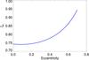 |
Fig. 6 Eccentricity factor ξe (see Eq. (68)) as a function of the eccentricity of the planetesimal. |
| In the text | |
|
Fig. 7 Contour plot of the decimal logarithm of the eccentricity focusing factors fe (see Eq. (70)) (in black) and fe,i (see Eq. (78)) (in red) as a function of orbital distance in a MMSN disk for dust of 1 mm in size. The eccentricity is the same as in Fig. 2. |
| In the text | |
|
Fig. 8 Illustration of dust capture in the settling regime. Planetesimals with a radius Rp between about 100 km and 1000 km have a Bondi radius larger than Rp but smaller than the Hill radius (see text). For the critical stopping time |
| In the text | |
|
Fig. 9 Value of the effective capture radius bset in units of the Bondi radius rB as a function of the ratio of the stopping time of the dust particle to the critical stopping time |
| In the text | |
|
Fig. 10 Contours of the logarithm of the gravitational focusing factor log 10(ffocus) (see Eq. (98)) as a function of dust size (in cm) and planetesimal size (in km), at 1 AU in the MMSN. The physical density of dust and planetesimals is set to 1 and 3 g cm-3, respectively. The different physical regimes (geometric, Safronov, settling, three-body) are identified by different colors. This figure assumes that planetesimals are on circular orbits. |
| In the text | |
|
Fig. 11 Illustration showing how gas streamlines (in black) are deflected around the planetesimal (at the center). The red streamlines correspond to dust particles with a stopping time that is on the same order as the interaction timescale. The thick red lines correspond to the most extreme streamlines leading to a collision, which define bhydro(τs). |
| In the text | |
|
Fig. 12 Value of fhydro as a function of the dimensionless friction time τf as obtained by Sekiya & Takeda (2003, their Fig. 8) (black line) and our fit (red line and Eq. (105)). |
| In the text | |
|
Fig. 13 Contours of the logarithm of the hydrodynamical factor log 10(fhydro) (see Eq. (105)) as a function of dust size (in cm) and planetesimal size (in km), at 1 AU in the MMSN. The physical density of dust and planetesimals is set to 1 and 3 g cm-3, respectively. The contours are for fhydro = 10-7, 10-6, 10-5, 10-0.5, 10-0.1. The transition from the hydrodynamic flow regime to the boundary regime (dark to light blue) takes place over a narrow range of dust sizes for planetesimals smaller than 100 km in radius. For larger planetesimal sizes, the transition between the hydrodynamic and settling regimes is discontinuous by construction. A proper modeling of this transition will require more work. |
| In the text | |
|
Fig. 14 Value of the turbulence factor ft (see Eq. (107)) as a function of dust size (in cm), at 1 AU in the MMSN for a turbulence viscosity parameter α = 10-2. We note that contrary to the other plots, the linear value of the factor is plotted instead of its log. |
| In the text | |
|
Fig. 15 2D collision probability |
| In the text | |
|
Fig. 16 Collision probability |
| In the text | |
|
Fig. 17 Same as Fig. 16, but with the collision probability |
| In the text | |
|
Fig. 18 Contours of the filtering efficiency by a MMSN planetesimal disk at 1 AU for α = 10-2, assuming monodisperse size distributions for planetesimals and dust grains. The contour indicating perfect filtering efficiency for log 10xfilter = 0 is shown in bold. |
| In the text | |
|
Fig. 19 Contours of the filtering efficiency by a MMSN planetesimal disk for 1 mm dust for α = 10-2, assuming a monodisperse size distribution for planetesimals. The contour indicating perfect filtering efficiency for log 10xfilter = 0 is shown in bold. |
| In the text | |
|
Fig. 20 Filtering efficiency of a swarm of planetesimals with radii between 1 km and 1000 km as a function of orbital distance and |
| In the text | |
|
Fig. 21 Filtering efficiency of dust of 1 micron to 100 meters by a MMSN planetesimal belt with planetesimals of 1 to 10 000 km in radius extending from 0.1 to 35 AU for a turbulent parameter α = 10-2 and assuming monodisperse size distributions for planetesimals and dust grains. Top panel: contours of the disk-integrated filtering factor Xfilter. Bottom panel: orbital distance at which Xfilter(r) = 1 for dust particles drifting in from beyond 35 AU. (The integration thus starts from 35 AU and goes inwards.) |
| In the text | |
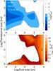 |
Fig. 22 Same as Fig. 21, but for a turbulent parameter α = 10-4. |
| In the text | |
|
Fig. C.1 Value of the effective capture radius bset in units of the Bondi radius rB from Eq. (90)(colored curves) together with the approximation used in Eq. (C.3)(thick black lines). Left panel: solution when the Bondi radius is smaller than the Hill radius. Right panel: solution when the Bondi radius is larger than the Hill radius (specifically, the solution of Eq. (90)is shown for RB/RH = 10). |
| In the text | |
|
Fig. C.2 Value of the collision probability |
| In the text | |
|
Fig. C.3 Value of the filtering efficiency log xfilter obtained by the full theory (black contours) and by the simplified one (red contours), for the MMSN and α = 10-4. The two panels are for two orbital distances: 0.1 AU (left) and 5 AU (right). (See Fig. C.2 for a full description.) |
| In the text | |
|
Fig. D.1 Contours of the filtering efficiency by a MMSN planetesimal disk at 1 AU for α = 10-4, assuming monodisperse size distributions for planetesimals and dust grains. The contour indicating perfect filtering efficiency for log 10xfilter = 0 is shown in bold. |
| In the text | |
|
Fig. D.2 Contours of the filtering efficiency by a MMSN planetesimal disk for 1 mm dust for α = 10-4, assuming a monodisperse size distribution for planetesimals. The contour indicating perfect filtering efficiency for log 10xfilter = 0 is shown in bold. |
| In the text | |
|
Fig. D.3 Filtering efficiency of a swarm of planetesimals with radii between 1 km and 1000 km as a function of orbital distance and mass of the gas disk for α = 10-4. (See Fig. 20 for details.) |
| In the text | |
|
Fig. E.1 Filtering efficiency of dust from 1 micron to 100 meters by a MMSN planetesimal belt with planetesimals of 1 − 10,000 km in radius extending from 0.1 to 35 AU for a turbulent parameter α = 10-4 and various ratios of the planetesimal to gas scale height, from an infinitely thin planetesimal disk with hp/hg = 0 (left panels), hp/hg = 0.1 (middle panels), and hp/hg = 1.0 (right panels). As in Figs. 21 and 22, the top panels show the contours of the disk-integrated filtering factor Xfilter while the bottom panels show the orbital distance at which Xfilter(r) = 1 for dust particles drifting in from beyond 35 AU. |
| In the text | |
Current usage metrics show cumulative count of Article Views (full-text article views including HTML views, PDF and ePub downloads, according to the available data) and Abstracts Views on Vision4Press platform.
Data correspond to usage on the plateform after 2015. The current usage metrics is available 48-96 hours after online publication and is updated daily on week days.
Initial download of the metrics may take a while.