| Issue |
A&A
Volume 572, December 2014
|
|
|---|---|---|
| Article Number | A61 | |
| Number of page(s) | 12 | |
| Section | Planets and planetary systems | |
| DOI | https://doi.org/10.1051/0004-6361/201322715 | |
| Published online | 28 November 2014 | |
Planet-vortex interaction: How a vortex can shepherd a planetary embryo
1 Heidelberg University, Center for Astronomy, Institute for Theoretical Astrophysics, Albert Ueberle Str. 2, 69120 Heidelberg, Germany
e-mail: sareh.ataiee@gmail.com
2 School of Astronomy, Institute for Research in Fundamental Sciences (IPM), Tehran, Iran
3 Department of Physics, Faculty of Sciences, Ferdowsi University of Mashhad, Mashhad, Iran
4 Institut für Astronomie & Astrophysik, Universität Tübingen, Auf der Morgenstelle 10, 72076 Tübingen, Germany
5 Konkoly Observatory, Research Center for Astronomy and Earth Science, Hungarian Academy of Sciences, Hungary
6 CEA, Irfu, SAp, Centre de Saclay, 91191 Gif-sur-Yvette, France
Received: 20 September 2013
Accepted: 26 September 2014
Context. Anti-cyclonic vortices are considered to be a favourable places for trapping dust and forming planetary embryos. On the other hand, they are massive blobs that can interact gravitationally with the planets in the disc.
Aims. We aim to study how a vortex interacts gravitationally with a planet that migrates towards the vortex or with a planet that is created inside the vortex.
Methods. We performed hydrodynamical simulations of a viscous locally isothermal disc using GFARGO and FARGO-ADSG. We set a stationary Gaussian pressure bump in the disc so that a large vortex is formed and maintained as a result of Rossby wave instability (RWI). After the vortex is established, we implanted a low-mass planet ([5,1,0.5] × 10-6M⋆) in the outer disc or inside the vortex and allowed it to migrate. We also examined the effect of vortex strength on the planet migration by doubling the height of the bump and checked the validity of the final result in the presence of self-gravity.
Results. We noticed that regardless of the planet’s initial position, the planet is finally locked to the RWI-created vortex in a 1:1 resonance or its migration is stopped at a larger orbital distance, in case of a stronger vortex. For the model with the weaker vortex (our standard model), we studied the effect of different parameters such as background viscosity, background surface density, mass of the planet, and different planet positions. In these models, while the trapping time and locking angle of the planet vary for different parameters, the main result, which is the planet-vortex locking, remains valid. We discovered that even a planet with a mass less than 5 × 10⁻⁷M⋆ comes out from the vortex and is locked to it at the same orbital distance. For a stronger vortex, both in non-self-gravitating and self-gravitating models, the planet migration is stopped far away from the radial position of the vortex. This effect can make the vortices a suitable place for continual planet formation under the condition that they save their shape during the planetary growth.
Key words: accretion, accretion disks / hydrodynamics / protoplanetary disks / planet-disk interactions
© ESO, 2014
1. Introduction
Theoretical models suggest that vortices can develop in protoplanetary discs and help solve timescale problems in the early planetary formation process and fast inward migration. The work by Li et al. (2000) provides the needed condition for Rossby wave instability (RWI) and vortex formation in protoplanetary discs. According to this work, a surface density change over a radial distance of the order of the disc scale-height is able to excite Rossby waves and eventually produce vortices. This condition can be provided by the disc spontaneously, for instance due to the presence of a dead-zone, or with the help of a gap-opening planet. Klahr & Bodenheimer (2003) showed that a protoplanetary disc with a radial gradient in the entropy becomes unstable and creates turbulence inside the disc. Owing to the turbulence-made pressure bumps, long-lasting vortices are formed. Vortices can also be established at the dead part of dead-zone edges because of a pile-up of matter due to different accretion rates (e.g. Regály et al. 2012; Lyra & Mac Low 2012). A massive planet, which opens a gap, can likewise produce a sufficiently steep density gradient at the gap edges and, therefore, vortices would be developed on both sides of the gap (e.g. Li et al. 2005; de Val-Borro et al. 2007; Ataiee et al. 2013; Fu et al. 2014).
It has been shown that anti-cyclonic vortices trap dust particles and boost planet formation (Barge & Sommeria 1995; Klahr & Henning 1997; Chavanis 2000; de La Fuente Marcos & Barge 2001; Johansen et al. 2004; Inaba & Barge 2006). The Coriolis force and the resultant higher pressure at the centre of anti-cyclonic vortices help to bring and accumulate dust particles inside the vortices (e.g. Zhu et al. 2014). In a pair of studies by Lyra et al. (2009a,b) the possibility of planet formation by vortices was studied. In the first work, they studied the planet formation at high pressure regions of a disc holding a Jupiter-mass planet in the presence of self-gravity. The results show that super-Earths can be formed inside the vortices generated at the outer edge of the gap. In the second work, they used a similar approach to study the formation and evolution of vortices created at the edge of a dead-zone and concluded that the dust accumulation inside vortices is so effective that objects of planetary mass can be formed in five orbits. Nevertheless, the effect of particle collision, erosion, or fragmentation has not been included in the mentioned work.
Anti-cyclonic vortices behave as “blobs” of matter and interact with planets in the disc. Koller et al. (2003) noticed that for small smoothing lengths in the potential of the planet, some vortices are formed out of the planet Roche lobe and propagated in the co-orbital region. They stated that the vortices exert significant torques on the planet. Li et al. (2009) and Yu et al. (2010) confirmed this statement by showing that the torques from the vortices created at the outer edge of a planet-carved gap in weakly viscous discs produce a slight outward migration of the planet.
If we consider vortices, as either a convenient birth place for planetary embryos or a mechanism for decreasing planetary migration rate, we introduce an important question: how does a planet embryo interact with a vortex? If the planet is formed inside a vortex, does it leave its birth place to allow further planetary formation in the vortex or does it stay until it becomes massive enough to open a gap? If a planet is made external to the vortex but during its migration meets the vortex, does it enter the vortex and disturb the planetary formation process? In this work, we aim to answer these questions by studying the migration of a low-mass planet in the presence of a stationary vortex created inside a Gaussian pressure bump. The order of the paper is as follows: In the next Sect. 2 we describe our model and the parameters used, we present our results in Sect. 3, discuss them in Sect. 4, and make conclusion in Sect. 5.
2. Method and setup
Pressure bumps, which are long-term pressure enhancements, are known as suitable traps for both particles and planets. Various processes such as accumulation of gas at the dead-zone edges or ice line (Kato et al. 2009), zonal flows (Johansen et al. 2009) or the outer edge of a gap created by a massive planet, can produce pressure bumps. Because of different drag forces felt by the particles at both sides of a pressure bumps, dust can drift towards the pressure maxima and grow (Haghighipour & Boss 2003; Johansen et al. 2007, 2011; Pinilla et al. 2012). On the other hand, low-mass planets that do not disturb the surface density much, are able to find a position in a bump where the differential Lindblad and co-rotation torques balance and hence are trapped (Lyra et al. 2009b). However, Regály et al. (2013) showed that, for slightly massive planets that can open a partial gap (at least 10 M⊕), trapping in a pressure maximum only occurs in the presence of a large-scale vortex. An RWI, which can be considered as the rotational equivalent of Kelvin-Helmholtz instability, may also be triggered in a pressure bump and produce anti-cyclonic vortices. Li et al. (2000) show that RWI can be excited if 10−20% radial density variation exists with a radial width not more than the thickness of the disc. The vortices created by RWI merge and form a single or a few large-scale vortices, which are appropriate places to trap and grow particles. This process can lead to planetesimal formation (Lyra et al. 2009b,a; Regály et al. 2012).
The question that arises here is: What would happen to a planet getting close to a vortex-holding bump or a planet-embryo that is created inside a vortex? We intend to answer this question by performing hydrodynamical simulations of discs that contain an embedded planet and a large vortex. We are interested in a large single vortex because (a) a large vortex is more probable of being observed than small vortices (an example of a possible observed vortex: van der Marel et al. 2013); (b) simulations show that RWI vortices are prone to merge into lower modes (e.g. Lyra et al. 2009b; Meheut et al. 2012a); and (c) analysing the torques between a planet and a single vortex is much easier than multiple vortices. We also study the effect of different parameters such as viscosity, planet mass and vortex strength.
Models with the parameters we studied.
2.1. Code
We performed our simulations with the GPU1 double-precision version of the FARGO code (Masset 2000) called GFARGO2. It is a Zeus-based code (Stone & Norman 1992) that solves Navier-Stokes equations with a full-viscous tensor implemented and continuity equation in a cylindrical coordinate system for a two-dimensional Keplerian disc at the presence of a central object and embedded planets. The continuity equation and the equation of motion read 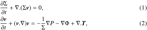 where v is the velocity vector, P is the pressure, and Φ is the gravitational potential of the star and planet. The potential Φ contains the indirect terms caused by the non-inertial coordinate system. In the case of a self-gravitating disc the corresponding accelerations are directly added to the righthand side of Eq. (2) (Baruteau & Masset 2008). The components of T, the viscous stress tensor, are given as
 ![\begin{eqnarray} && T_{rr}= 2 \Sigma \nu \left[\frac{\partial v_{\rm r}}{\partial r} - \frac{1}{3} \left(\nabla . \vec{v}\right) \right],\\ && T_{\theta \theta} = 2 \Sigma \nu \left[\frac{1}{r} \frac{\partial v_{\theta}}{\partial \theta} + \frac{v_{\rm r}}{r} - \frac{1}{3} \left(\nabla . \vec{v}\right) \right], \\ && T_{r\theta} = T_{\theta r} = \Sigma \nu \left[r \frac{\partial}{\partial r}\left(\frac{v_{\theta}}{r}\right) + \frac{1}{r} \frac{\partial v_{\rm r}}{\partial \theta} \right]\cdot \end{eqnarray}](/articles/aa/full_html/2014/12/aa22715-13/aa22715-13-eq45.png) The isothermal equation of state is applied with a radial temperature profile, which is determined through the aspect ratio or an arbitrary radial sound speed profile.
The isothermal equation of state is applied with a radial temperature profile, which is determined through the aspect ratio or an arbitrary radial sound speed profile.
We modified the code to enable us: (a) to insert a planet into the simulation at our desired time and angular position; (b) to set up a steady Gaussian bump for the viscosity; and (c) to start the velocity perturbation at a specific time. In this code, the calculations are performed in a coordinate system that is centred on the star. In the model massive vortex (SG), where we tested the effect of self-gravity, we used FARGO-ADSG which is capable of handling disc self-gravity and adiabatic thermodynamics.
To assure our results are not code-dependent, we tested some of our models independently with the code RH2D (Kley 1989, 1999). The results of the both codes were identical.
2.2. Numerical setup for the standard model
We considered a locally isothermal disc with constant background surface density ![\hbox{$\Sigma_{\rm BG}=5 \times 10^{-4}\ [M_{\star}/r_{0}^2]$}](/articles/aa/full_html/2014/12/aa22715-13/aa22715-13-eq46.png) and kinematic viscosity
and kinematic viscosity ![\hbox{$\nu_{\rm BG}=10^{-5}\ [r_{0}^2 \Omega_{\rm k}(r_{0})]$}](/articles/aa/full_html/2014/12/aa22715-13/aa22715-13-eq47.png) where Ωk is Keplerian angular velocity. To avoid singular behaviour in the gravitational potential of the planet, we used a smoothing parameter ϵ = 0.6H(rp) as
where Ωk is Keplerian angular velocity. To avoid singular behaviour in the gravitational potential of the planet, we used a smoothing parameter ϵ = 0.6H(rp) as  (6)where Mp = 5 × 10⁻⁶M⋆ is the mass of the planet that is equivalent to 1.7 MEarth in a system with a solar mass star. We used a fixed non-rotating 2D polar coordinate (r,θ) with 256 logarithmic grids in radial and 512 equidistant grids in azimuthal direction. The disc was extended from 0.5r0 to 1.5r0 and the wave-damping boundary condition (de Val-Borro et al. 2006) was applied to both inner and outer boundaries. In the models in which we initially start with the planet inside the vortex, the planet was introduced after 300 orbits when a large vortex was formed. In the rest of the models, the planet was introduced to the disc at the beginning, but its potential was slowly switched on during the first ten orbits. We continued the simulations until the planet passed the bump and reached the inner boundary or until it was trapped inside the bump for more than 1000 orbits.
2.3. Making a vortex
In order to produce a single vortex and study its interaction with a planet, we need to have a controlled formation condition that enables us to understand the effect of each parameter. For instance, because of continuous gas accumulation at the edge of a dead-zone, the different parameters of the density bump, such as height and width, are changing in time and consequently influence the vortex (e.g. Regály et al. 2013). Therefore, we embedded a Gaussian density bump, corresponding to a pressure bump in a locally isothermal disc, into a smooth disc and altered the disc and planet properties while we used fixed values for the width and position of the bump. To prevent the bump from smoothing out in time, we adjusted the viscosity profile to provide a physical mechanism in the system for the higher surface density in the bump. Specifically, we prescribed the following fixed profile for the viscosity:  (7)where νBG(r) is the background viscosity of the disc, a is the height of the bump that controls the amount of density/viscosity enhancement/reduction in the bump, and r0 represents the location of the bump in the disc and is used as the length scale in our simulations. Finally, c controls the width of the bump. A dead-zone edge, where a viscosity reduction or enhancement happens, can be considered a more realistic example of such density-viscosity adaptation (Lyra et al. 2009b). The disc was considered flat with the constant aspect ratio h = 0.05. In the main models, the bump parameters are fixed to a = 1 and c = H(r0) = h(r0)r0 = 0.05 with H(r) being the pressure scale-height. The exception to this are some test models in which we examine the effect of vortex strength on the planet migration. Our choice of c = 0.05 is the marginal value for RWI formation based on the threshold presented by Li et al. (2000). For a wider bump, we do not expect vortex formation. We tested this criterium in the test model Width06 (see Table 1), and the result in Fig. 1 shows no vortex even after 4000 orbits.
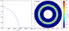 |
Fig. 1 Semi-major axis evolution (left) and surface density at t = 4000 orbits for Width06. Because of a wide bump, no vortex is formed. |
We set up a Gaussian density profile, Σ(r) in consideration of the imposed viscosity profile, at the start of the simulations ![\begin{equation} \label{dens} \Sigma(r) = \Sigma_{\rm BG}(r) \left[1+a\ \exp\left(-\frac{(r-r_{0})^2}{2 c^2}\right)\right] \cdot \end{equation}](/articles/aa/full_html/2014/12/aa22715-13/aa22715-13-eq67.png) (8)We ignited the RWI with subsequent vortex formation either by adding an initial perturbation to the radial velocity inside the bump or by the planet itself. In the models without an initial planet inside the disc, we added an initial random perturbation,
(8)We ignited the RWI with subsequent vortex formation either by adding an initial perturbation to the radial velocity inside the bump or by the planet itself. In the models without an initial planet inside the disc, we added an initial random perturbation,  (9)to the radial velocity3 where rand(1) is a function that produces a random number between 0 and 1. Our choice of random initial perturbation prevents the excitation of a specific mode. Because of our specific set-up for the bump, the vortex neither gets destroyed nor migrates. In the cases with the planet initially inside the disc but outside of the bump, the perturbation, which excites the RWI and triggers subsequent vortex formation, is created by the planet.
Although these two different methods might result in different initial azimuthal positions and shapes of a single vortex, the final trapping position of the planet relative to the vortex was not affected by the initialization method. A typical outcome of our simulations (here the standard model) is shown in Fig. 2, where we compare the density distribution of two runs with and without initial velocity perturbation (after Eq. (9)), and the migration history of an embedded planet of mass Mp = 5 × 10⁻⁶M⋆. The planet was initialized at a distance rp = 1.2r0.
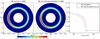 |
Fig. 2 Comparison between two models: one where the vortex formation is ignited by the planet (left), and one where it is excited by the radial velocity perturbation (middle). The left and middle panels show the surface density after 600 orbits when a single vortex has been established. In the right panel, ap is the variation of planet semi-major axis. |
2.4. Resolution
To optimize the resolution considering run-time and numerical convergence, we repeated our standard model (nr × ns = 256 × 512) with two higher resolution models (HR1 and HR2 models in Table 1). We compared the half-horseshoe width xHS with the cell width at the bump using the relation by Paardekooper et al. (2010a) for low-mass planets. The half-horseshoe width was resolved by ~3, ~6 and ~9 cells in the standard, HR1 and HR2 models, respectively. Figure 3 shows that while the resolution can affect the migration rate and the trapping time, it does not change the trapping position and long-term behaviour of the planet. Paardekooper et al. (2010a) showed that the models with half-horseshoe width resolved through six cells are in good agreement with the analytical calculations. Moreover, Fig. 3 presents identical trapping positions for our standard and higher resolution models. Thus, we are assured that the co-rotation torque is resolved for all numerical resolution. Therefore, we applied the resolution of our standard model to the rest of the simulations.
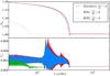 |
Fig. 3 Effect of numerical resolution on the planet migration (upper panel) and planet eccentricity (lower panel). The trapping position of the planet is not sensitive to the resolution while the trapping time can vary. In HR2, because the outer boundary is at 1.3 (Table 1), we set the planet slightly inward of the other two models to avoid numerical issues. |
2.5. Parameters under study
We studied how the trapping of the planet is changed because of the variation of some physical parameters such as background viscosity, background surface density, planet mass, and different initial position of the planet. We altered the background viscosity between 10-5, 10-6 and 10-7, which corresponds to α = 4 × 10⁻³, 4 × 10⁻⁴ and 4 × 10⁻⁵ in α-prescription of viscosity (Shakura & Sunyaev 1973). We chose a lower ΣBG = 10-4 and a higher 10-3 background surface density than the standard model. Because the vortex can be a suitable place for producing planet embryos, we tried lower planet masses Mp = 1 × 10⁻⁶ and 5 × 10⁻⁷ (equivalent to 0.3 and 0.17 Earth mass in a solar-like system ) with their initial position inside the vortex to have an estimation of embryos mass that can stay inside a vortex. Because the value of horseshoe drag is affected by the resolution, we adjusted the radial span to always keep the resolution (xHS/ Δr ~ 3) equal to the standard model. To check if the final trapping position of the planet depends on the initial position of the planet, we repeated the standard model with the planet in different positions towards the vortex. Table 1 summarizes the important parameters of all models.
3. Results
3.1. Standard model
The red line in Fig. 3 shows the evolution of the semi-major axis of the planet in our standard model. The planet is started out of the bump at rinit = 1.2r0 and migrates towards the bump. Due to a steeper surface density slope in the outer part of the bump, the planet migrates faster when it approaches the vortex, and after a severe interaction with the vortex at ~3000 orbits it is trapped by the vortex. Not only is the planet trapped by the vortex, but it is also locked to it by keeping a constant distance from the vortex centre (≈90 degrees from the vortex centre). One might find this result in contradiction with Regály et al. (2013) in which they showed a temporary trapping of the planet. In their work, they studied a 10 M⊕ planet, which opened a partial gap and therefore destroyed the vortex as it came close to it. Because our study deals with low-mass planets that do not open a gap and also a vortex that is long-lived, the planets are trapped permanently.
Checking the dependency of the results on the initial planet position, we examined 16 test models with the planets implanted slightly outward or inward of the vortex radial position and different azimuth towards the vortex centre. In these simulations, we saved the outputs every 1/10th of an orbit to follow the planet path precisely. We named the models with the planet initialized at ai = 1.05r0, On − models and those with the planet at ai = 0.95r0, In − models where n represents the planet-vortex azimuthal difference. We found that while the planet is radially trapped in a similar position to the standard model, the locking side can be either trailing or leading. As seen in Table 2, no relation can be found between the initial position of the planet and the final locking side. In Fig. 5, we display the surface density of four models and below each panel, we draw the corresponding path of the planet from the times marked in Fig. 6. The final locking position seems to be given by the relative position of the planets upon close approach that cannot be predicted a priori.
Final azimuthal position of the planet in O and I models.
To see what happens for a planet that is born and becomes massive inside a vortex, we started the simulation by implanting the planet inside the vortex. In the upper panel of Fig. 4, we track the planet’s motion in a frame co-rotating with the vortex. The planet gradually leaves the vortex and never enters back into it, while oscillating around a specific location where it is trapped eventually. We plotted the semi-major axis of the planet in the lower panel of Fig. 4. It shows that the planet migrates inward and then outward during the first 100 orbits. After that, the planet oscillates radially around a position where it stays until the end of the simulation. We sketch the orbital evolution of the planet in the illustration in Fig. 4.
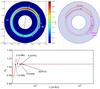 |
Fig. 4 Planet trapping in the frame co-rotating with the vortex. The left upper panel demonstrates a planet initially set inside the vortex (position 0), which comes out and moves to the position 1 and then returns back to 2. Afterwards, it oscillates around position 5 until it is locked to the vortex at this location. We illustrate the planet’s behaviour in the right upper panel in a more exaggerated way to show the radial migration of the planet as well. The lower panel shows the semi-major axis of the planet by time. The numbers denote the times of the marked positions in the left upper panel. We marked the positive and negative torques from the vortex by the + and − signs. The indirect torque from the star has the opposite sign of the vortex torque (Sect. 4). |
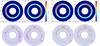 |
Fig. 5 Upper panels demonstrate the final trapping positions of two O-models (left panels) and two I-models (right panels). In the lower panels, we draw the path of the planet from the times marked in Fig. 6 with “O” and “I” until they are trapped. For clarity, we exaggerated the description of the migration of the planets. |
3.2. Parameter study
Figure 7 shows the results for discs with different background viscosity. While the semi-major axis of the trapped planet is nearly the same for all cases, the azimuthal distance between the planet and the vortex centre differs when altering the viscosity. This can be explained by considering the shape of the vortices. As the viscosity decreases, the vortex becomes more elongated. Therefore, the planet, which is locked to the tail of the vortex, is located farther from the vortex-centre. The lower panel of Fig. 7 shows that the planet migration rate and trapping time also depend on the background viscosity. In all of our models with the planet starting outside of the bump, the planet’s inward migration is accelerated as it approaches the bump. This happens because both of the Lindblad and vortensity-related component of co-rotation torques becomes more negative as the result of steeper surface density (see Kley & Nelson 2012; Paardekooper et al. 2010a, for more detail). Different migration rates are the consequence of co-rotation torque saturation (see Baruteau & Masset 2013, as a good review).
The background surface density is another parameter we altered to see whether the mass of the vortex has a destabilizing effect. Figure 8 displays the evolution of planet semi-major axis in discs with different background surface densities. In the case with the highest value ΣBG = 10-3, the migration is faster and the planet is trapped after a stronger interaction with the vortex compared to the standard model. For the lowest background surface density ΣBG = 10-4, the planet migrates more slowly, but is eventually trapped.
Figure 9 shows that the three stages of migrating inward, outward and oscillating around the trapping position exist for lower planet masses as well. Although the oscillating time is longer for less massive planets, all of them get finally trapped.
4. Discussion and torque analysis
4.1. Dominant torque components
To understand the reason why the planet locks to the vortex, either to its head or tail, we need to figure out which torques are exerted on the planet and which ones play the main role. Usually, in disc models with axisymmetric background, Lindblad and co-rotation torques4 determine the migration of a planet. In the presence of a non-axisymmetric feature in the disc or a massive companion, the barycentre of the system is shifted away from the star and therefore, in the centre of mass frame, the star exerts a torque on the planet due to its displacement from the barycentre. The schematic view of the star and the vortex torques are shown in Fig. 10. In the code, the calculation is done in the coordinate frame centred on the star. The asymmetric feature in the disc accelerates the star by shifting the barycentre away and consequently, an indirect torque is exerted on the planet because of the accelerated coordinate frame. This indirect term in the accelerated frame is equivalent to the star torque in the centre of mass frame and we will use them interchangeably for the convenience. We note that the vortex produces an azimuthal density gradient in the co-orbital region of the planet that might also modify the co-rotation contribution in the disc torque.
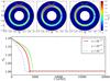 |
Fig. 7 Trapping of the planet in discs with different background viscosity. The upper panels demonstrate the locking position of the planet towards the centre of the vortex. The lower panel shows the change of planet semi-major against time. |
We choose the Visc1 model for torque analysis and generalise the discussion to the rest of the models. The Visc1 model, which is the standard model with ν = 10-6, is an intermediate model considering the vortex length. In order to study the torques on the planet more easily, we repeated the model with ν = 10-6 in a co-rotating frame. The indirect torque is given by 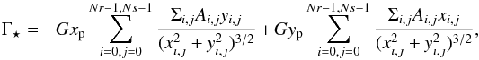 (10)where Ai,j is the area of the cell [i,j]. In the co-rotating frame, the second term vanishes and xp = ap. The disc torque Γdisc is the gravitational torque from all disc cells on the planet in the frame centred on the star.
Figure 11 displays the star torque and the disc torque on the planet. The torques are normalised to Γ0, which is defined as 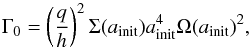 (11)where Σ(ainit) and Ω(ainit) are the surface density and Keplerian angular velocity at the initial location of the planet (ainit = 1.2r0), and q represents the ratio of the planet mass to the star mass. The figure shows that when the planet is far from the vortex orbit, the disc exerts an oscillating torque on the planet because of the changing distance between the vortex and the planet. Because the system’s barycentre is also rotating around the coordinate centre, the star torque oscillates too. After about 5000 orbits, the disc torque and the star torque balances and the planet is trapped.
 |
Fig. 8 Evolution of planet semi-major axis for different background surface densities. The higher amplitude and longer oscillation of the planet semi-major axis before trapping shows the stronger interaction between the planet and the vortex in the case with Σ = 10-3. |
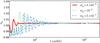 |
Fig. 9 Evolution of planet semi-major axis for different planet masses. |
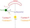 |
Fig. 10 Star and vortex torque on the planet in a coordinate centred on the barycentre. The distance between the barycentre and the star is much smaller than shown. This drawing illustrates the physics of our model rather than the code calculations. |
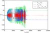 |
Fig. 11 Normalised torques from the disc (Γdisc) and the star (Γ⋆) on the planet in the model with ν = 10-6. The solid line represents the net torque from both the disc and the star. The stellar and the disc torques are always opposite in sign. |
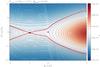 |
Fig. 12 Surface density and streamlines for the Visc6 model for the trapped planet. The thick red line is the separatrix around the horseshoe region of the planet. The + and × demonstrate the position of the planet and stagnation point, respectively. The distances from the planet (R − a) are scaled by the Hill radius of the planet (RH). |
While the balance of stellar and disc torques explains the radial location of the final trapping, the locking location in azimuth, here to the tail of the vortex, needs to be discussed. To answer this question, we need to find out how different torque components depend on the azimuthal position of the planet. The torques on the planet are derived from Lindblad resonances, co-rotation and horseshoe region, the vortex, and the star displacement.
In Fig. 12, we show the area around the planet’s orbit in more detail, including streamlines and horseshoe region. The spirals emanating from the planet, starting above and below the + symbol in Fig. 11, give rise to the Lindblad torques. The Lindblad torque arises from the location of the inner and outer Lindblad resonances, which can be shifted by different parameters, such as surface density or deviation of the velocity profile from Keplerian. On the other hand, the vortex changes the velocity profile of the neighbouring gas and pushes the open streamlines farther away in comparison with the no-vortex case (see deformation of streamlines outside of the red line in Fig. 12). According to the definition of the Lindblad resonances (where the gas angular frequencies in the planet’s co-moving frame match the epicyclic frequencies), they cannot exist inside the vortex or horseshoe region where the streamlines are closed. To estimate the Lindblad torque after planet locking, we repeated the model with ν = 10-6 in the co-rotating frame with a fixed planet located at the trapping position. Figure 13 shows the radial torque distribution for t = 100 orbits and at the end of the simulation. The green area, which is denoted by 2xs, shows the analytically calculated horseshoe width and can be considered as the width of the horseshoe region before the vortex formation. The area coloured in orange represents the larger horseshoe width at the end of the simulation. The Lindblad resonances contribution comes from the sum of torque values outside of the horseshoe region. If we consider the orange area as the horseshoe width and integrate the red curve in Fig. 13 over the radii outside of the horseshoe region, it provides us an estimate for the Lindblad torque. This value is ΓL/ Γ0 ≃ 5, which is ~15% of the total torque and shows that while the Lindblad torque is considerable, the main component of the torque belongs to the torque from the horseshoe region.
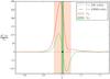 |
Fig. 13 Radial torque distribution scaled by Γ0 for the Visc1 (FP) model. The green and red lines represent the torque distribution before the vortex was developed and at the end of the simulation. The green area exhibits the analytically calculated horseshoe region for our planet in an axisymmetric disc. The orange area shows the larger horseshoe width obtained from Fig. 12. The position of the planet is also marked by a black dot. We note that we only plotted the torque from the disc and thus the integral of the red curve, which is non-zero, equal to −Γ⋆. |
The presence of the vortex both deforms the horseshoe region (red line in Fig. 12) and exerts an extra torque on the planet. The horseshoe width is much larger on the vortex side than the width on the other side. Not only does the asymmetric horseshoe region cause a large co-rotation torque on the planet, but the asymmetric azimuthal density distribution also produces a torque with the same sign as the co-rotation torque (positive in this case). Hence, the presence of the vortex inside the horseshoe region changes the torques such that the planet can be captured by the vortex. The vortex torque and co-rotation torque cannot be calculated separately because they are tightly related. To estimate the contributions of the vortex and co-rotation torques, we subtract the density at t = 100 orbits, before the vortex formation, from the surface density at the end of the simulation in order to obtain the density enhancement due to the vortex. Then, we calculate the vortex gravitational torque on the planet in the co-rotating frame using the relation below: 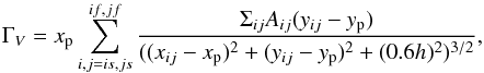 (12)where [is,if] and [js,jf] represent the cell indices of radial and azimuthal extension of the vortex. We estimate the vortex radial and azimuthal extension based on the density reduction as 1.7 of the background value. We note that this value is chosen in a way that could describe the shape of the vortex well enough. Because we were only interested in an estimation of the vortex mass, this simple method fits our aim. We avoid the singularity around the planet by adding the smoothing parameter 0.6h to the calculation. Using this method, the vortex torque contribution equals to ΓV/ Γf ≃ 18%. The rest of the final torque, which is ≃67%, originates from the co-rotation torque.
The star torque is also a function of planet azimuth. It can be easily understood in the frame centred on the barycentre (see Fig. 10). As the planet rotates around the star, the angle between the star force F⋆ and planet position vector  changes. Because the torque depends on the sine of this angle, star torque has its maximum value where the planet azimuth towards the vortex is π. In Fig. 14, we calculated and plotted the star torque and the vortex torque as a function of planet azimuth. As the results show, the distance between azimuthal locking position of the planet and the vortex is not necessarily π, but it depends on the extent of the vortex.
As the results of O and I models show, both end of the vortex wings are stable points. On the leading side, the vortex and co-rotation torques are negative and the star torque is positive. In contrast, on the trailing side, the vortex and co-rotation torques are positive and start torque is negative. How the planet chooses the leading or trailing side is unclear to us, but we think that the planet is trapped where it succeeds to adjust its horseshoe orbit to the vortex streamlines. Because the locking side of the planet has no observational consequence or influence on planet formation, we leave the investigation of this point to future study.
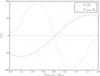 |
Fig. 14 Star torque and vortex torque as a function of azimuthal distance between the planet and the vortex centre for the Visc1 model. |
Similar torque analysis can be applied to the other models too. For example, in the model with a planet started at the vortex centre, the planet initially migrates due to the Lindblad torques arisen from the Lindblad resonances out of the vortex. We note that while the co-rotation torque and the torque from the vortex can not exist inside the vortex (because the vortex is dominated to the planet horseshoe streamlines), the condition for the Lindblad resonances can be fulfilled outside of the vortex, where the gas elements do not have closed orbits. Because the vortex centre is not a stable point, the planet comes out of the vortex (refer to Appendix A for supplementary discussion). The migration of the planet continues until it reaches the point where the planet, star and vortex centre are located on a straight line. Similar to the vortex centre, this point is not an equilibrium position owing to the Lindblad torques. After that, the battle between the inward and outward migration continues until the planet finds the right place where the co-rotation, vortex and Lindblad torque can cancel out the torque from star.
4.2. Strength of the vortex
To examine whether a more massive vortex is able to trap a planet, we re-ran the standard model with a = 2, which contained more mass inside the bump. The yellow line in Fig. 15 represents the semi-major axis of the planet against time. In this case, the plant is “prevented” from inward migration instead of being trapped. In Fig. 16, we display the star, disc and net torques on the planet. After averaging the net torque over the last 4000 orbits, we plotted this value by the black thin solid line. This figure shows that after the planet inward migration is stopped, the average net torque on the planet is almost zero whereas the net torque at each time does not vanish.
We indicated the azimuthal distance between the planet and the vortex in three different positions in Fig. 16. Two of them refer to the positions where the disc torque has the maximum and minimum values. The third position is where the disc torque is nearly zero. When the vortex is after the planet (θv − p = 0.54), the disc torque is large and positive. As the vortex rotates and crosses the opposite side of the planet (θv − p = 3.45), the disc torque becomes about zero. And when the vortex comes close to the planet from behind, the disc torque changes to a large negative value. The dependency of the sign and the value of the disc torque on the vortex position shows that in this model, the main torque on the planet is due to the gravitational torque of the vortex. Therefore, if the vortex is strong enough, the vortex can play the main role in halting the migration of the planet even if it is not located inside the horseshoe region.
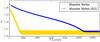 |
Fig. 15 Semi-major axis evolution for the standard models, except with double height for the bump (Height2 models). The yellow and blue lines represent the model with and without self-gravity, respectively. |
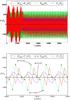 |
Fig. 16 Upper panel: scaled torque risen from disc and star on the planet for model Height2. The red and black (thin) solid lines represent the net torque and the time averaged torque, respectively. Lower panel: shorter section of time between [4505 − 4525] orbits. θv − p in this figure, denotes the azimuthal distance between the vortex and the planet. This value is given for three different times: 4512.9, 4517.15 and 4515.15 orbits. |
Whether self-gravity (SG) alters the results of the Height2 model is an important question. Lovelace & Hohlfeld (2013) analytically studied the stability condition in thin discs with grooves or bumps at the presence of self-gravity. They showed that discs becomes unstable for the axisymmetric perturbation if Q> (π/ 2)(r0/H), or equivalently Q(H/r0) >π/ 2, where Q = κcs/πGΣ is Toomre parameter (Toomre 1964), and  is the epicyclic frequency. We plotted QH as a function of r before the vortex formation in Fig. 17. This plot indicates that SG might play a role in this model.
To directly test the effect of SG in this case, we repeated an identical simulation with the self-gravitating version of FARGO. First, we note that the vortex still exits in the SG case. With SG the vortex is more elongated but weaker, i.e. the density at the centre of the vortex in this case is lower than in the model without SG. Moreover, Q is much higher than unity even at the centre of vortex (see Fig. 18). Then, we followed the evolution of an embedded planet that started at a0 ≃ 1.2. The blue line in Fig. 15 shows the semi-major axis of the planet for the SG model. Although the migration is slower than the Height2 model because of the disc self-gravity (Pierens & Huré 2005), the planet again does not reach the vortex, but its inward migration stops, because of the gravitational interaction between the vortex, the star and the planet. In Fig. 18, we plotted the surface density and Toomre parameter at t = 13 000 orbits for the model, with and without SG.
As Table 3 suggests, the locking or stopping of the planet depends on the surface density at the vortex centre. In the table, we compared the properties of the vortices in different models. The models Visc2 and Dens1 have the most massive vortices because of the very elongated shape in the first model and the higher surface density in the second model. The planet migration is not stopped in either of the two models. On the other hand, Height2 and Height2 (SG) models have the highest surface density at the centre of their vortices, and the planet migration is halted farther away from the vortices in both of them. This comparison shows the surface density at the vortex centre is an important factor in different trapping behaviour of the planet. When the planet comes close to the vortex centre, it exchanges torque with the vortex centre and if the torque is large enough, it migrates outward, as in the Height2 models. Because the torque of star and vortex on the planet scale with planet mass while the Linblad torque scales with planet mass squared, a turnover point in the planet’s migration behaviour as a function of the planet mass is expected. For planet masses larger than a critical value, the planet could not be expelled by the vortex any more. We leave the detailed analysis of this point to a future study because it is beyond the scope of this paper.
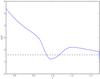 |
Fig. 17 Toomre value multiplied by the disc scale-height QH for the Height2 model as a function of radius. Q is calculated at before the vortex formation. The dotted black line shows the critical value π/ 2. |
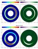 |
Fig. 18 Upper and lower panels respectively present the surface density Σ and Toomre parameter Q for the Height2 (top) and Height2 (SG) (bottom) models at t = 13 000 orbits, when the planet migration has been halted. |
The formation of one massive large-scale vortex in the self-gravitated model might appear in contradiction with the result of some other works (e.g. Mamatsashvili & Rice 2009) that indicate the vortices sizes are limited by the Jeans scale of the disc. This different behaviour can be attributed to our specified viscosity profile, which maintains the RWI and vortex formation continuously. Mamatsashvili & Rice (2009) argues that the combined effect of self-gravity and Keplerian shear opposes the merging of vortices or destructs the large-scale vortices into smaller vortices. However, in Lyra et al. (2009a), who use a setup more similar to ours both in viscosity reduction and locally isothermal equation of state, large vortices (m = 3) with Q ≈ 1 are formed at t = 75 orbits. Because in our model, (a) the energy dissipation can not occur because we omitted the energy equation; (b) the RWI is continuously driven by the fixed-shaped bump and the planet; and (c) the simulations are performed for a large number of orbits, the large-scale vortex is formed and survives.
In Fig. 19, we compared the evolution of different modes of density Fourier transform for self-gravitating and non-self-gravitating models. We expanded the density at the bump tip Σmax(θ) as  (13)and plotted the difference between Σm and the initial density Σ0 as a function of time. In both models, the higher modes are dominant initially, but all of them have equal amplitudes. Later, all lower modes grow and finally m = 1 becomes the strongest. After the linear growth phase, all modes have smaller amplitude in the SG model than the non-SG model. Another important point is that the growth happens at a later time for the SG model. This is in agreement with the results of Lin (2012) and Lin & Papaloizou (2011), which study the effect of self-gravity on the vortices formed at the edge of a gap and show that the self-gravity delays merging of vortices. In our models, although we do not see merging because of mixing the modes, the postponing of vortices growth due to the self-gravity can be clearly observed. We defer a more detailed study of vortices in SG discs to future work.
Vortex properties for different models.
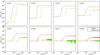 |
Fig. 19 Comparison of different modes between Height2 and Height2 (SG) models. |
5. Summary and conclusion
We studied the interaction between a low-mass planet (upto q = 5 × 10⁻⁶) and a 2D large-scale stationary vortex formed in a viscously stable Gaussian pressure bump. Whether such bumps really do exist in protoplanetary discs is still an open question whose definite answer needs a higher resolution observation. However, the ring structures in transitional discs can be considered strong evidence for the presence of pressure bumps and even vortices (e.g. Brown et al. 2009; Casassus et al. 2013; van der Marel et al. 2013). Numerical simulations of discs with gap-opening planets show that in a very weakly viscous discs, a density bump as high as ~1.8 times of the background density can be created (Crida et al. 2006). Another probable situation is very narrow viscosity transition in an outer dead-zone edge. In the 2D simulations of Regály et al. (2013), the density is raised to five times of the background value, but at a wider distance than the thickness of the disc. If the width of viscosity transition becomes narrower, a bump similar to our models may be created.
Our results show that in all of our basic models the planet migrates towards the vortex, interacts with it, and eventually is locked to the vortex in an identical radial distance and at a specific angular position far from the vortex centre. The locking position is determined by the balance between the torque from the vortex, star, and the local disc. We noticed that if the vortex becomes stronger, the planet exhibits different behaviour. Instead of “locking”, it is “stopped” and its migration is halted farther away from the vortex position.
We also set up a planet inside the vortex in some of our models and we discovered that the planet is expelled out of the vortex during the first hundreds orbits and afterward the planet is locked to one side of the vortex. It can even happen for a planet as low mass as 5 × 10⁻⁷M⋆. This has two consequences: on the positive side, the vortex can serve as a “womb” and continue producing more planetary cores, one after another, and on the negative side, the planetary core is ejected by the vortex and could not grow to higher mass values.
We caution that in this work we introduced the planet suddenly inside the vortex. Meheut et al. (2012b) show that large dust particles can greatly affect their parent vortices. Thus, a more complete work is needed to answer the question of whether a vortex can maintain its shape while growing a planet. Another weakness of our work is that we could not study whether a low-mass planet has a role in vortex destruction. This question will be answered in Regály & Sándor (in prep.).
We performed our models for a fixed pressure bump, and consequently a fixed vortex in a flat disc. In more realistic models, the vortex could migrate (Paardekooper et al. 2010b), move in the disc (Regály et al. 2013), or even be threatened by decay (e.g. Meheut et al. 2012a). It is very interesting to explore whether a moving vortex in a more realistic disc is able to “lay a planet system” or not. We will try to answer this question in future works.
The co-rotation torque has two components: linear and non-linear (or horseshoe drag). Paardekooper & Papaloizou (2008) showed that the nonlinear component, if unsaturated, can dominate the migration of the planet. Therefore, when we use the term co-rotation torque in this work, we mean the horseshoe drag.
Acknowledgments
We thank P. Pinilla for the fruitful discussions, F. Masset for his kind help in interpreting GFARGO output files, and J. Ramsey for his kind help in maintaining the GPUs in Institute for Theoretical Astrophysics. This work was financed partly by a scholarship of the Ministry of Science, Research, and Technology of Iran, and partly by the 3rd funding line of the German Excellence Initiative. Zs. Regály has been supported by the Lendület-2009 Young Researcher’s Program of the Hungarian Academy of Sciences, City of Szombathely under agreement No.K-111027 and Hungarian grant K-101393.
References
- Ataiee, S., Pinilla, P., Zsom, A., et al. 2013, A&A, 553, L3 [NASA ADS] [CrossRef] [EDP Sciences] [Google Scholar]
- Barge, P., & Sommeria, J. 1995, A&A, 295, L1 [NASA ADS] [Google Scholar]
- Baruteau, C., & Masset, F. 2008, ApJ, 678, 483 [NASA ADS] [CrossRef] [Google Scholar]
- Baruteau, C., & Masset, F. 2013, in Lect. Not. Phys. 861, eds. J. Souchay, S. Mathis, & T. Tokieda (Berlin: Springer Verlag), 201 [Google Scholar]
- Brown, J. M., Blake, G. A., Qi, C., et al. 2009, ApJ, 704, 496 [NASA ADS] [CrossRef] [Google Scholar]
- Casassus, S., van der Plas, G., Perez, S. M., et al. 2013, Nature, 493, 191 [NASA ADS] [CrossRef] [Google Scholar]
- Chavanis, P. H. 2000, A&A, 356, 1089 [NASA ADS] [Google Scholar]
- Crida, A., Morbidelli, A., & Masset, F. 2006, Icarus, 181, 587 [Google Scholar]
- de La Fuente Marcos, C., & Barge, P. 2001, MNRAS, 323, 601 [Google Scholar]
- de Val-Borro, M., Edgar, R. G., Artymowicz, P., et al. 2006, MNRAS, 370, 529 [NASA ADS] [CrossRef] [Google Scholar]
- de Val-Borro, M., M., Artymowicz, P., D’Angelo, G., & Peplinski, A. 2007, A&A, 471, 1043 [NASA ADS] [CrossRef] [EDP Sciences] [Google Scholar]
- Fu, W., Li, H., Lubow, S., & Li, S. 2014, ApJ, 788, L41 [NASA ADS] [CrossRef] [Google Scholar]
- Haghighipour, N., & Boss, A. 2003, ApJ, 598, 1301 [NASA ADS] [CrossRef] [Google Scholar]
- Inaba, S., & Barge, P. 2006, ApJ, 649, 415 [NASA ADS] [CrossRef] [EDP Sciences] [Google Scholar]
- Johansen, A., Andersen, A. C., & Brandenburg, A. 2004, A&A, 417, 361 [NASA ADS] [CrossRef] [EDP Sciences] [Google Scholar]
- Johansen, A., Oishi, J. S., Mac Low, M.-M., et al. 2007, Nature, 448, 1022 [Google Scholar]
- Johansen, A., Youdin, A., & Klahr, H. 2009, ApJ, 697, 1269 [NASA ADS] [CrossRef] [Google Scholar]
- Johansen, A., Klahr, H., & Henning, T. 2011, A&A, 529, A62 [NASA ADS] [CrossRef] [EDP Sciences] [Google Scholar]
- Kato, M. T., Nakamura, K., Tandokoro, R., Fujimoto, M., & Ida, S. 2009, ApJ, 691, 1697 [NASA ADS] [CrossRef] [Google Scholar]
- Klahr, H., & Bodenheimer, P. 2003, ApJ, 582, 869 [NASA ADS] [CrossRef] [Google Scholar]
- Klahr, H. H., & Henning, T. 1997, Icarus, 229, 213 [NASA ADS] [CrossRef] [Google Scholar]
- Kley, W. 1989, A&A, 208, 98 [NASA ADS] [Google Scholar]
- Kley, W. 1999, MNRAS, 303, 696 [NASA ADS] [CrossRef] [Google Scholar]
- Kley, W., & Nelson, R. P. 2012, ARA&A, 50, 211 [NASA ADS] [CrossRef] [Google Scholar]
- Koller, J., Li, H., & Lin, D. 2003, ApJ, 596, L91 [NASA ADS] [CrossRef] [Google Scholar]
- Li, H., Finn, J., & Lovelace, R. 2000, ApJ, 533, 1023 [NASA ADS] [CrossRef] [Google Scholar]
- Li, H., Li, S., Koller, J., et al. 2005, ApJ, 624, 1003 [NASA ADS] [CrossRef] [Google Scholar]
- Li, H., Lubow, S. H., Li, S., & Lin, D. N. C. 2009, ApJ, 690, L52 [NASA ADS] [CrossRef] [Google Scholar]
- Lin, M.-K. 2012, MNRAS, 426, 3211 [NASA ADS] [CrossRef] [Google Scholar]
- Lin, M.-K., & Papaloizou, J. C. B. 2011, MNRAS, 415, 1426 [NASA ADS] [CrossRef] [Google Scholar]
- Lovelace, R. V. E., & Hohlfeld, R. G. 2013, MNRAS, 429, 529 [NASA ADS] [CrossRef] [Google Scholar]
- Lyra, W., & Mac Low, M.-M. 2012, ApJ, 756, 62 [NASA ADS] [CrossRef] [Google Scholar]
- Lyra, W., Johansen, A., Klahr, H., & Piskunov, N. 2009a, A&A, 493, 1125 [NASA ADS] [CrossRef] [EDP Sciences] [Google Scholar]
- Lyra, W., Johansen, A., Zsom, A., Klahr, H., & Piskunov, N. 2009b, A&A, 497, 869 [NASA ADS] [CrossRef] [EDP Sciences] [Google Scholar]
- Mamatsashvili, G. R., & Rice, W. K. M. 2009, MNRAS, 394, 2153 [NASA ADS] [CrossRef] [Google Scholar]
- Masset, F. 2000, A&AS, 141, 165 [NASA ADS] [CrossRef] [EDP Sciences] [Google Scholar]
- Masset, F. S. 2011, Celest. Mech. Dyn. Astron., 111, 131 [Google Scholar]
- Meheut, H., Keppens, R., Casse, F., & Benz, W. 2012a, A&A, 542, A9 [Google Scholar]
- Meheut, H., Meliani, Z., Varniere, P., & Benz, W. 2012b, A&A, 545, A134 [NASA ADS] [CrossRef] [EDP Sciences] [Google Scholar]
- Paardekooper, S., & Papaloizou, J. C. B. 2008, A&A, 895, 877 [NASA ADS] [CrossRef] [EDP Sciences] [Google Scholar]
- Paardekooper, S.-J., Baruteau, C., Crida, A., & Kley, W. 2010a, MNRAS, 401, 1950 [NASA ADS] [CrossRef] [Google Scholar]
- Paardekooper, S.-J., Lesur, G., & Papaloizou, J. C. B. 2010b, ApJ, 725, 146 [NASA ADS] [CrossRef] [Google Scholar]
- Pierens, A., & Huré, J. 2005, A&A, 433, L37 [NASA ADS] [CrossRef] [EDP Sciences] [Google Scholar]
- Pinilla, P., Birnstiel, T., Ricci, L., et al. 2012, A&A, 538, A114 [NASA ADS] [CrossRef] [EDP Sciences] [Google Scholar]
- Regály, Z., Juhász, A., Sándor, Z., & Dullemond, C. P. 2012, MNRAS, 419, 1701 [NASA ADS] [CrossRef] [Google Scholar]
- Regály, Z., Sándor, Z., Csomós, P., & Ataiee, S. 2013, MNRAS, 433, 2626 [NASA ADS] [CrossRef] [Google Scholar]
- Shakura, N. I., & Sunyaev, R. A. 1973, A&A, 24, 337 [NASA ADS] [Google Scholar]
- Stone, J., & Norman, M. 1992, ApJS, 80, 753 [Google Scholar]
- Toomre, A. 1964, ApJ, 139, 1217 [NASA ADS] [CrossRef] [Google Scholar]
- van der Marel, N., van Dishoeck, E. F., Bruderer, S., et al. 2013, Science, 340, 1199 [NASA ADS] [CrossRef] [PubMed] [Google Scholar]
- Yu, C., Li, H., Li, S., Lubow, S. H., & Lin, D. N. C. 2010, ApJ, 712, 198 [NASA ADS] [CrossRef] [Google Scholar]
- Zhu, Z., Stone, J. M., Rafikov, R. R., & Bai, X.-N. 2014, ApJ, 785, 122 [NASA ADS] [CrossRef] [Google Scholar]
Appendix A: Torques at the vortex centre
On a planet inside a vortex, only Lindblad, vortex gravitational, and star torques can play role. The co-rotation torque needs the horseshoe orbits, which can not be formed inside the vortex because of the circulation of material inside the vortex. Therefore, this component can be ignored until the planet comes out of the vortex.
The Lindblad torque is calculated by summing the individual torques from each Lindblad resonances. Masset (2011) showed that the Lindblad torque is not very sensitive to the second derivative of surface density. Therefore, we used the analytical formula by Paardekooper et al. (2010a) to estimate the maximum Lindblad torque in every position of the disc with a symmetric bump. Figure A.1 shows the Lindblad torque on the planet calculated by  (A.1)where α = −dlog Σ/dlog r and β = −dlog T/ dlog r, which equals 1 in our models. We calculated α numerically at each r over the azimuthally averaged surface density. The figure shows that the scaled Lindblad torque equals to −2 for a planet at the bump centre. Based on the definition of Lindblad torques that uses the epicylic frequency, in our models, the Lindblad resonances can be formed outside of the vortex and consequently farther away from the planet. This can even lower the normalised Lindblad torque Γ/Γ0 to a value less than −2.
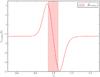 |
Fig. A.1 Maximum Lindblad torque at planet orbital position. The torque is calculated using relation (A.1) and the radial density profile of the disc before vortex formation. The Lindblad torque has the highest value when planet is close to the bump edges. The pink area shows the vortex radial extension in the bump after it formed. These values are calculated for the Visc1 model. |
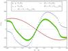 |
Fig. A.2 Normalised star and vortex gravitational torques on the planet at different azimuthal position towards the vortex centre at the bump maxima. The green solid line represents the sum of the two components. The dashed and dotted lines demonstrate the variation of the total torque by the Lindblad torque. The maximum and minimum values of the Lindblad torque are obtained from Fig. A.1. The horizontal axis is limited to the vortex azimuthal extension. |
To calculate the star and vortex gravitational torques, we put the planet at different azimuth with respect to the vortex centre at the bump maximum and calculated these two components for Visc6 model. Noting that the Lindblad torque is much smaller than the vortex gravitational and star torques, it can only shift the zero torque position to the right (trailing) or left (leading) of vortex centre. As Fig. A.2 shows, if the planet is displaced slightly to the right of the vortex centre, the positive torque causes outward migration and if the planets moves slightly to the left, the negative torques bring the planet out of vortex. Except for the Lindblad torques, which has minor effect in our models (see the green area in Fig. A.2), all the other normalised torque components are independent of planet mass. Figuring out the lowest mass planet that can remain inside the vortex is a question that can be answered by studying the planet formation from dust to planet which is not the scope of this paper.
All Tables
All Figures
|
Fig. 1 Semi-major axis evolution (left) and surface density at t = 4000 orbits for Width06. Because of a wide bump, no vortex is formed. |
| In the text | |
|
Fig. 2 Comparison between two models: one where the vortex formation is ignited by the planet (left), and one where it is excited by the radial velocity perturbation (middle). The left and middle panels show the surface density after 600 orbits when a single vortex has been established. In the right panel, ap is the variation of planet semi-major axis. |
| In the text | |
|
Fig. 3 Effect of numerical resolution on the planet migration (upper panel) and planet eccentricity (lower panel). The trapping position of the planet is not sensitive to the resolution while the trapping time can vary. In HR2, because the outer boundary is at 1.3 (Table 1), we set the planet slightly inward of the other two models to avoid numerical issues. |
| In the text | |
|
Fig. 4 Planet trapping in the frame co-rotating with the vortex. The left upper panel demonstrates a planet initially set inside the vortex (position 0), which comes out and moves to the position 1 and then returns back to 2. Afterwards, it oscillates around position 5 until it is locked to the vortex at this location. We illustrate the planet’s behaviour in the right upper panel in a more exaggerated way to show the radial migration of the planet as well. The lower panel shows the semi-major axis of the planet by time. The numbers denote the times of the marked positions in the left upper panel. We marked the positive and negative torques from the vortex by the + and − signs. The indirect torque from the star has the opposite sign of the vortex torque (Sect. 4). |
| In the text | |
|
Fig. 5 Upper panels demonstrate the final trapping positions of two O-models (left panels) and two I-models (right panels). In the lower panels, we draw the path of the planet from the times marked in Fig. 6 with “O” and “I” until they are trapped. For clarity, we exaggerated the description of the migration of the planets. |
| In the text | |
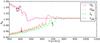 |
Fig. 6 Semi-major axis evolution of four selected models displayed in Fig. 5. |
| In the text | |
|
Fig. 7 Trapping of the planet in discs with different background viscosity. The upper panels demonstrate the locking position of the planet towards the centre of the vortex. The lower panel shows the change of planet semi-major against time. |
| In the text | |
|
Fig. 8 Evolution of planet semi-major axis for different background surface densities. The higher amplitude and longer oscillation of the planet semi-major axis before trapping shows the stronger interaction between the planet and the vortex in the case with Σ = 10-3. |
| In the text | |
|
Fig. 9 Evolution of planet semi-major axis for different planet masses. |
| In the text | |
|
Fig. 10 Star and vortex torque on the planet in a coordinate centred on the barycentre. The distance between the barycentre and the star is much smaller than shown. This drawing illustrates the physics of our model rather than the code calculations. |
| In the text | |
|
Fig. 11 Normalised torques from the disc (Γdisc) and the star (Γ⋆) on the planet in the model with ν = 10-6. The solid line represents the net torque from both the disc and the star. The stellar and the disc torques are always opposite in sign. |
| In the text | |
|
Fig. 12 Surface density and streamlines for the Visc6 model for the trapped planet. The thick red line is the separatrix around the horseshoe region of the planet. The + and × demonstrate the position of the planet and stagnation point, respectively. The distances from the planet (R − a) are scaled by the Hill radius of the planet (RH). |
| In the text | |
|
Fig. 13 Radial torque distribution scaled by Γ0 for the Visc1 (FP) model. The green and red lines represent the torque distribution before the vortex was developed and at the end of the simulation. The green area exhibits the analytically calculated horseshoe region for our planet in an axisymmetric disc. The orange area shows the larger horseshoe width obtained from Fig. 12. The position of the planet is also marked by a black dot. We note that we only plotted the torque from the disc and thus the integral of the red curve, which is non-zero, equal to −Γ⋆. |
| In the text | |
|
Fig. 14 Star torque and vortex torque as a function of azimuthal distance between the planet and the vortex centre for the Visc1 model. |
| In the text | |
|
Fig. 15 Semi-major axis evolution for the standard models, except with double height for the bump (Height2 models). The yellow and blue lines represent the model with and without self-gravity, respectively. |
| In the text | |
|
Fig. 16 Upper panel: scaled torque risen from disc and star on the planet for model Height2. The red and black (thin) solid lines represent the net torque and the time averaged torque, respectively. Lower panel: shorter section of time between [4505 − 4525] orbits. θv − p in this figure, denotes the azimuthal distance between the vortex and the planet. This value is given for three different times: 4512.9, 4517.15 and 4515.15 orbits. |
| In the text | |
|
Fig. 17 Toomre value multiplied by the disc scale-height QH for the Height2 model as a function of radius. Q is calculated at before the vortex formation. The dotted black line shows the critical value π/ 2. |
| In the text | |
|
Fig. 18 Upper and lower panels respectively present the surface density Σ and Toomre parameter Q for the Height2 (top) and Height2 (SG) (bottom) models at t = 13 000 orbits, when the planet migration has been halted. |
| In the text | |
|
Fig. 19 Comparison of different modes between Height2 and Height2 (SG) models. |
| In the text | |
|
Fig. A.1 Maximum Lindblad torque at planet orbital position. The torque is calculated using relation (A.1) and the radial density profile of the disc before vortex formation. The Lindblad torque has the highest value when planet is close to the bump edges. The pink area shows the vortex radial extension in the bump after it formed. These values are calculated for the Visc1 model. |
| In the text | |
|
Fig. A.2 Normalised star and vortex gravitational torques on the planet at different azimuthal position towards the vortex centre at the bump maxima. The green solid line represents the sum of the two components. The dashed and dotted lines demonstrate the variation of the total torque by the Lindblad torque. The maximum and minimum values of the Lindblad torque are obtained from Fig. A.1. The horizontal axis is limited to the vortex azimuthal extension. |
| In the text | |
Current usage metrics show cumulative count of Article Views (full-text article views including HTML views, PDF and ePub downloads, according to the available data) and Abstracts Views on Vision4Press platform.
Data correspond to usage on the plateform after 2015. The current usage metrics is available 48-96 hours after online publication and is updated daily on week days.
Initial download of the metrics may take a while.