| Issue |
A&A
Volume 571, November 2014
|
|
|---|---|---|
| Article Number | A79 | |
| Number of page(s) | 14 | |
| Section | Astrophysical processes | |
| DOI | https://doi.org/10.1051/0004-6361/201424641 | |
| Published online | 14 November 2014 | |
Scattering line polarization in rotating, optically thick disks
1 UMR 7293 J.L. Lagrange Laboratory, Université de Nice Sophia Antipolis, CNRS, Observatoire de la Côte d’Azur, Campus Valrose, 06108 Nice, France
e-mail: milic@aob.rs
2 Astronomical observatory Belgrade, Volgina 7, 11060 Belgrade, Serbia
Received: 21 July 2014
Accepted: 14 September 2014
Context. To interpret observations of astrophysical disks, it is essential to understand the formation process of the emitted light. If the disk is optically thick, scattering dominated and permeated by a Keplerian velocity field, non-local thermodynamic equilibrium (NLTE) radiative transfer modeling must be done to compute the emergent spectrum from a given disk model.
Aims. We investigate NLTE polarized line formation in different simple disk models and aim to demonstrate the importance of both radiative transfer effects and scattering, as well as the effects of velocity fields.
Methods. We self-consistently solve the coupled equations of radiative transfer and statistical equilibrium for a two-level atom model by means of Jacobi iteration. We use the short characteristics method of formal solution in two-dimensional axisymmetric media and compute scattering polarization, that is Q/I and U/I line profiles, using the reduced intensity formalism. We account for the presence of Keplerian velocity fields by casting the radiative transfer equation in the observer’s frame.
Results. Relatively simple (homogeneous and isothermal) disk models show complex intensity profiles that owe their shape to the interplay of multidimensional NLTE radiative transfer and the presence of rotation. The degree of scattering polarization is significantly influenced not only by the inclination of the disk with respect to observer, but also by the optical thickness of the disk and the presence of rotation. Stokes U/I shows double-lobed profiles with amplitude that increases with the disk rotation.
Conclusions. Our results suggest that the line profiles, especially the polarized ones, emerging from gaseous disks differ significantly from the profiles predicted by simple approximations. Even in the case of the simple two-level atom model, we obtain line profiles that are diverse in shape, but typically symmetric in Stokes Q and antisymmetric in Stokes U. A clear indicator of disk rotation is the presence of Stokes U, which might prove to be a useful diagnostic tool. We also demonstrate that, for moderate rotational velocities, an approximate treatment can be used, where NLTE radiative transfer is done in the velocity field-free approximation, and Doppler shift is applied in the process of spatial integration over the whole emitting surface.
Key words: line: formation / radiative transfer / polarization / methods: numerical
© ESO, 2014
1. Introduction
Interpreting spectroscopic and spectropolarimetric observations of different kinds of gaseous disks relies on the understanding of the process of spectral line formation. Disks that scatter incoming radiation and/or emit by themselves are often encountered: circumstellar and circumbinary disks, protoplanetary disks, accrection disks on different scales, etc. It is not rare that understanding the role of the disk is crucial for a proper interpretation of the observations. The best known example is probably the unified model of active galactic nuclei as a result of detection of scattering polarization in spectral lines by Antonucci & Miller (1985). Another case where the presence of a disk proved essential is the explanation of the presence of emission lines in Be stars (for a recent review of the subject, see Rivinius et al. 2013) by the process of light scattering on the gaseous disk that surrounds the star.
Although modern radiative transfer techniques are almost routinely employed in solar and stellar physics (for a review, see, for example, Carlsson 2009), detailed radiative transfer computations of line transfer in astrophysical disks are rarely found in the modern literature. Adam (1990) and Papkalla (1995) were among the first to employ numerical radiative transfer techniques in order to self-consistently solve the non-local thermodynamic equilibrium (NLTE) line formation problem in multi-dimensional disk models. A study of scattering line polarization in disks has been conducted by Ignace (2000), but was limited to optically thin case, i.e. neglecting radiative transfer effects taking place in the disk. Vink et al. (2005) used Monte Carlo simulations to investigate line scattering in rotating circumstellar disks. In their model, the disk is illuminated by a host star. They found that the presence of the “gap” between the surface of the star and the inner boundary of a rotating disk changes the way the degree of rotation of polarization plane varies with wavelength across the line profile. Recently, Wheelwright et al. (2012) have confronted high-quality spectropolarimetric observation with detailed radiative transfer modeling (see also Carciofi et al. 2009; Carciofi & Bjorkman 2008). Another recent study, conducted by Halonen et al. (2013) deals with the polarization of the continuum radiation in realistic disk models and demonstrates that it depends strongly both on the inclination of the disk and on the wavelength. We also want to draw attention to the work of Dessart & Hillier (2011) who deal with a different topic (polarization in the supernovae ejecta) but are relevant to this work because they also consider axial symmetry and the effects of scattering.
Concerning the importance of detailed radiative transfer (RT) computations of spectral line formation, Elitzur et al. (2012) have demonstrated the need for understanding the role of NLTE (i.e., line scattering) processes. Their main conclusion is that the double-peaked profiles, which are usually assumed to be an indicator of disk rotation, may occur simply due to the gradient of the source function (that is, the emission coefficient) along the line of sight. It is well known from the theory of stellar atmospheres that scattering processes can cause these source function gradients, even in an isothermal medium. Another important consequence of line scattering is the so-called scattering polarization. It is linear polarization, resulting from uneven population of Zeeman sublevels. It is further influenced by weak magnetic fields (Hanle effect). Scattering polarization and Hanle effect are routinely exploited in solar magnetic field diagnostics (see, for example, Trujillo Bueno et al. 2004) where very complex and detailed formalism is utilized to compute the emergent Stokes vector.
To the authors’ knowledge, the formalism of NLTE polarized line transfer (the ultimate reference in the field is the monograph by Landi Degl’Innocenti & Landolfi 2004) has not yet been applied to polarized line formation in gaseous astrophysical disks. Here we attempt to take the first steps in such an investigation. We self-consistently solve the radiative transfer and statistical equilibrium equations in the presence of line scattering in order to compute emergent polarized line profiles. We restrict ourselves to the case of a two-level atom line transfer and to axisymmetric disk models. Our primary aim is not to obtain maximum realism but rather to investigate the importance of radiative transfer effects and disk rotation on emerging line profiles. We thus, in this paper, restrict ourselves to idealized, homogeneous (in the context of this work meaning: constant opacity), isothermal disk models. One is to keep in mind that even in these very simple cases, we are faced with the interplay of radiative transfer effects in optically thick media, non-LTE effects, multidimensionality effects, and the influence of the disk differential rotation. As we see in the remainder of the paper, all of these effects leave a significant imprint on the emerging line shape and line polarization.
In Sect. 2 we outline the NLTE problem of the second kind and the method of solution. In Sects. 3 and 4 we present results for self-emitting and illuminated disks, respectively. In Sect. 5 we draw some conclusions and discuss possible directions for future work.
2. Method
We are interested in obtaining the emergent polarized intensity from the disk as a whole. What we observe is spatially (and, in case of photometry, frequency-) integrated intensity, or, in general, Stokes vector. To compute the total disk radiation, one has to compute the specific emergent intensity and to perform spatial integration over the whole emitting surface.
The majority of the recent works dealing with disk-like objects utilize Monte Carlo methods to compute disk images or SED (spectral energy distribution) curves. However, they are mostly aimed at computing the continuum radiation, as well as self-consistent disk temperature distribution. We are interested in a different process, line scattering, so we consider the disk model (opacity and temperature distribution) to be given; that is, we assume that spectral lines do not influence the energy balance of the object significantly. We compute the emergent intensity by solving the radiative transfer equation (RTE), which in the most general case reads as 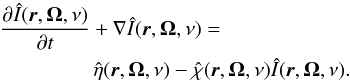 (1)Here Î is the polarized intensity given as the Stokes vector (I,Q,U,V)†,
  is the emission coefficient (also a four-vector), and
  is the 4 × 4 absorption matrix. Also, Ω = (θ,ϕ) is the direction of the propagation and ν the radiation frequency.
We assume axial symmetry and thus cast the radiative transfer equation in a 2D cylindrical coordinate system (z,r). In the case where we also introduce a Cartesian coordinate system, the z axis coincides with the axis of the cylinder while the disk lies in the xy plane. We are interested in obtaining the emergent polarized intensity at the top boundary of the disk (z = ztotal), since we restrict ourselves to disks that are geometrically thin (i.e., rtotal ≫ ztotal, where subscript “total” refers to the size of the disk along the appropriate coordinate) so the emitting surface is actually the top boundary.
To obtain the emergent (generally, polarized) intensity, we need to solve the radiative transfer equation. Here, and depend on the populations of the atomic energy levels, which in turn depend on temperature and density, but also on the radiation field itself, which brings inevitable coupling in the radiative transfer problem. We will present the way of dealing with this problem under the following assumptions:
-
We restrict ourselves to time-independent (stationary) problemand to axisymmetric objects. We thus cast the radiative transferequation in 2D cylindrical coordinate system.The spatial dependence of all the quantities is given by z and r coordinates, where z goes from zero to ztotal, where ztotal corresponds to the top boundary of the disk, and r goes from zero to rtotal, where r = 0 refers to the center of the disk.
-
We assume that line transport is taking place in a two-level atom model where the lower level of the transition is unpolarized. Under this assumption the absorption matrix takes the form
 , where 1 is unit matrix. The two-level atom assumption is adequate for resonance lines. Polarized line formation process for transitions requiring multilevel treatment (such as Hα) is much more complex. but the main effects outlined in this work should manifest themselves similarly.
 -
We consider a magnetic field − free case. That means that there is no Hanle effect (see Ignace 2010, for optically thin computations of Hanle effect in disks) and that Stokes Q and U arise thanks to the anisotropy of the radiation. Using the formalism from Anusha & Nagendra (2011b), we can easily implement the Hanle effect of large scale magnetic fields in our computations (but note that the magnetic field would have to be axisymmetric). Also, we neglect any Zeeman effect; i.e., Stokes V is identical to zero.
With these assumptions, χ does not depend on the direction any more. We divide Eq. (1) with −χ and use the so-called along-the-ray form of the radiative transfer equation to get ![\begin{equation} \frac{{\rm d} \hat{I}(z,r, \vec{\Omega}, \nu)}{{\rm d} \tau} = \phi(\nu) \left [\hat{I} (z,r,\vec{\Omega}, \nu) - \hat{S}(z,r,\vec{\Omega}, \nu)\right] .\label{RTE} \end{equation}](/articles/aa/full_html/2014/11/aa24641-14/aa24641-14-eq29.png) (2)Here, Ŝ is known as the source function, the ratio between emission and absorption coefficient, and φ(ν) is the line absorption profile, which describes the dependence of the line opacity on frequency. The variable τ is known as the line-integrated optical depth along the ray, that is,
(2)Here, Ŝ is known as the source function, the ratio between emission and absorption coefficient, and φ(ν) is the line absorption profile, which describes the dependence of the line opacity on frequency. The variable τ is known as the line-integrated optical depth along the ray, that is, 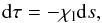 (3)where χl is the line-integrated absorption coefficient and ds is the elementary path along the ray. Here the “ray” is a line with the orientation given by the angle Ω, along which the radiative transfer equation is integrated. Under the assumption of complete frequency redistribution in the line scattering process (frequencies of incoming and outgoing photons are uncorrelated), the source function becomes independent of frequency and has the following form:
  (4)where ϵ is the photon destruction probability, ϵ = Cul/ (Aul + Cul); Aul and Cul are the upper-level radiative and collisional lifetime, respectively;
  where B is equal to the local Planck function at the frequency ν; Ŵ is a diagonal matrix whose elements account for the intrinsic line polarizability and depolarization due to the presence of elastic collisions and/or unresolved, randomly oriented magnetic field. The variable
  is known as the scattering matrix, which describes correlations between incoming and outgoing photons. Equation (4) is known as the equation of statistical equilibrium for a two-level atom.
The smaller the rate of collisions (Cul) with respect to the radiative rate (Aul), the greater the importance of the scattering processes and the source function differs more from the local Planck function. For high rate of collisions, the source function is practically identical to the local Planck function, and this situation is known as local thermodynamic equilibrium or LTE. The importance of departures from LTE (NLTE) is a well known problem in the field of stellar atmospheres (Mihalas 1978). The non-LTE case, generalized to the problem of line scattering polarization, is known as the “NLTE problem of the second kind” (for a recent review, see, for example Trujillo Bueno 2009).
We need a self-consistent solution of coupled Eqs. (2) and (4) on a 2D (z,r) grid, under the assumption of axial symmetry and some assumed angular and frequency discretization. A detailed description of a numerical solution in this kind of geometry is given in Milić (2013), where the NLTE problem of the second kind is cast in the so-called real reduced intensity formalism first introduced by Frisch (2007) and generalized to 3D geometry by Anusha & Nagendra (2011a). In the next section we briefly recap the reduced intensity formalism and refer the interested reader to works cited above.
2.1. Reduced intensity formalism
It can be shown (Frisch 2007; Anusha & Nagendra 2011a) that both the polarized source function Ŝ and the polarized intensity Î can be decomposed by using the so-called real reduced source function and reduced intensity ( and
and  , respectively):
  (5)and
  (6)where
  and ℐ are the real reduced source function and intensity, and the matrices
  and
and  are linear operators that relate the reduced formalism and the Stokes formalism. The reduced formalism results from the expansion of the scattering phase matrix on the irreducible spherical tensors
  basis (see Landi Degl’Innocenti & Landolfi 2004, for details). The explicit form is given by Frisch (2007) for 1D media and by Anusha & Nagendra (2011a) for the general, 3D case. The main advantage of this approach is that the reduced source function is now angle independent, which significantly increases the efficiency of numerical codes used for the solution of the NLTE problem of the second kind. The reduced intensity and reduced source function obey the same form of radiative transfer equation,
 ![\begin{equation} \frac{{\rm d}\hat{\cal I}(z,r, \vec{\Omega}, \nu)}{{\rm d} \tau} = \phi(\nu) \left [\hat{I} (z,r,\vec{\Omega}, \nu) - \hat{\cal S}(z,r)\right], \label{rrRTE} \end{equation}](/articles/aa/full_html/2014/11/aa24641-14/aa24641-14-eq56.png) (7)while the statistical equilibrium equation has the form
(7)while the statistical equilibrium equation has the form 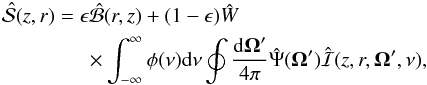 (8)where Ψ(Ω′) is the scattering matrix in the real reduced formalism. The problem of coupled Eqs. (7) and (8) is formally identical to the standard (i.e., unpolarized) NLTE radiative transfer problem, and with appropriate changes, one can use the same numerical scheme to solve it. Once the self-consistent solution has been found, one can compute Stokes components of interest from the real reduced intensities (see Anusha & Nagendra 2011a, for the exact form of the transformation).
We solve the problem of the coupled equations of radiative transfer and statistical equilibrium by using Jacobi iteration. This method is based on casting Eq. (2) (or, in the polarized case, Eq. (7)) in an integral form and introducing the so-called Λ operator so that![\begin{equation} \hat{\cal S} = \epsilon \hat{B} + (1-\epsilon) \hat{\Lambda} [\hat{\cal S}]. \end{equation}](/articles/aa/full_html/2014/11/aa24641-14/aa24641-14-eq60.png) (9)In Jacobi iteration,
(9)In Jacobi iteration,  is split into a local (diagonal) and a non-local part. The local part is easily inverted and the errors introduced by this approximation are iteratively corrected. For a detailed review of the subject, see Hubeny (2003) and for applications of Jacobi iteration and similar techniques to polarized NLTE radiative transfer see Trujillo Bueno (2003). The details for applying Jacobi iteration to the polarized line formation in reduced intensity formalism for this specific geometry are given in Milić (2013).
For the research conducted here, we have slightly changed the formal solution (way of computing the specific intensity from a given value of the source function) scheme used in Milić (2013) so it now corresponds to BESSER (Štěpán & Trujillo Bueno 2013) formal solution, which utilizes second-order, smooth and monotonic interpolation technique. We have also employed BESSER interpolation for the spatial and angular interpolation needed to perform the formal solution along the ray. We also use the subgridding strategy proposed by van Noort et al. (2002) and subsequently by Ibgui et al. (2013). This enables more precise computation of the monochromatic optical path along the ray in the observer’s reference frame (see next section).
2.2. Velocity fields
To compute the emergent spectrum for rotating disks, one must properly account for the rotation of the disk. In the case of rigid body rotation, any two points on the disk do not move with respect to the other. That means that the radiative transfer can be done in the static case, and radiation from different parts of the disk can be added together afterwards (see Sect. 3.1). A more realistic and, from the radiative transfer point of view, more problematic case is when the gas in the disk is following a Keplerian velocity distribution: 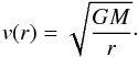 (10)Or, if we define the rotational velocity v0 at radius r0, then
  (11)Now the situation is clearly different from the rigid body rotation because any two points in the disk are moving with respect to each other. Since the radiative transfer problem is a spatially coupled problem (i.e., the radiation field in one point depends on the radiation field in other points), Doppler shifts resulting from this relative movement must be taken into account. Here, we have used the observer-frame formalism (see, e.g., Mihalas 1978), where all the relevant quantities are expressed in the coordinate frame of the observer. All the equations keep the same form, but frequencies and directions become coupled. For example, the opacity coefficient (and, subsequently, the optical path distance between two points) is now also direction-dependent, as
  (12)where
  (13)Here s = (sinθcosϕ,sinθsinϕ,cosθ) and v = (vx,vy,vz), while the observer is assumed to be situated in (0,0,0).
This formalism is straightforward and powerful, because it allows for including arbitrary velocity fields but suffers from computational inefficiency when high velocities come into play since it requires the use of a frequency mesh that covers all possible Doppler shifts. For rapidly rotating disks, this might easily render the computation fairly cumbersome. However, it turns out that the relevant quantity is not the velocity itself but rather the ratio of the velocity to the Doppler velocity of the gas. To clarify this, we use the reduced frequency scale instead of regular frequency, i.e., substitute ν with f:  (14)where ΔνD = ν0vD/c is known as the Doppler width of the line, vD is then the Doppler velocity which accounts for all the random, small-scale velocities of the gas (thermal velocities of constituting atoms and small scale turbulent velocities). Equation (12) now takes the form
  (15)where
  is the velocity given in units of the Doppler velocity. It is clear now that the relative Doppler shift is what is important. Therefore, high random velocities can suppress the effect of rotation and, in principle, of any systematic velocity field. This statement is an extremely important thing to keep in mind. Here we restrict ourselves to the case of moderate rotational velocities (vrot ≈ 10vD). This is because we are primarily interested in the study of circumstellar disks, but the results and our main points should be applicable to faster rotating disks as well. This regime of intermediate velocities is particularly interesting because velocities are high enough to influence the line formation process1, but still not high enough to justify the Sobolev approximation or similar high-velocity regimes.
To have some idea of the velocities we consider here, one should keep in mind that the thermal velocity of hydrogen atoms on temperatures of ≈104 K is around 10 km s-1. Turbulent gas motions could increase this velocity somewhat, which means that the rotational velocities considered in the next chapter are on the order of 100 km s-1. If we consider a typical UV or optical line with λ = 300 − 800 nm, one Doppler width would correspond to ≈0.01 nm, which requires a spectral resolution of a few times 104.
3. Results
In this section we show the results of applying the method described above to two models of gaseous disks. Both are homogeneous and isothermal. First, we consider disks that are completely self-emitting, i.e. the light of the central body is neglected. The other type are disks that have a star in the center. In our computations we incorporate the starlight in the boundary conditions corectly for the radiative transfer problem but do not add the light from the part of the star that is not occulted by the disk to the total flux. In the rest of the chapter we comment further on both of the models.
Before inspecting the profile shapes for different disk models, it is important to realize that the velocity field influences the emergent spectrum in two ways: i) first, the velocity gradient, if large enough, can alter the distribution of the source function in the object, as the photons can escape the medium more easily. ii) The gradient of the velocity field along a line of sight causes Doppler shifts, thus changing the effective depth up to which the medium is probed 2. For moderate velocities like this, we expect the second effect to be dominant.
However, we first investigate the decrease in the source function due to the loss of photons because of the velocity gradient. We consider a disk model with its radial line-integrated optical thickness τr equal to 1000 and vertical optical thickness τz equal to 10. We set χ0 = 1 and thus the geometrical grid is identical to the optical depth grid. The Planck function is set to unity (i.e., the disk is isothermal), and the photon destruction probability is equal to ϵ = 10-4 everywhere in the disk. In this and all other computations, we assume a Doppler line absorption profile; i.e.,  . We do not account for continuum opacity; i.e., we are only interested in the line radiative transfer. Also, as the opacity is constant, we use the optical depth as the relevant “spatial” coordinate. In the rest of the text, the optical depth/thickness of the disks is computed from the so-called mean or line integrated opacity, χ0.
The disk is rotating according to the following law:  (16)for r>rc, where rc = rtotal/ 10 and
  (17)for r<rc. That is, the disk is rotating like a solid body in the inner 10% part of the radius (this is to avoid very large velocities for small values of the radius) and with a Keplerian law elsewhere. For now, we assume that the disk is emitting only by itself; i.e., the radiation of the central object is assumed to be negligible.
We self-consistently compute the polarized source function both in the static case and the case where v(rtotal) = 5vD and compare the values of  (first component component of the reduced source function, which is, to a good approximation, identical to the first component of the Stokes source function, SI) between the two cases. The 2D distribution of the source function in both cases is shown in Fig. 1. Here the total optical thickness along the z and r coordinates is equal to 10 and 103, respectively. Although the optical thickness is substantial and far from the optically thin case, the object is effectively thin; i.e. the optical thickness of the medium along both axis is much smaller than the thermalization length for the line source function. (SI would be equal to the Planck function at optical depths on the order of 1 /ϵ.)
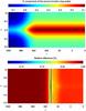 |
Fig. 1 2D distribution of SI source function in the z,r plane for the non-rotating cylinder (up) and relative difference between rotating and static case (down). The source function is given in units of the Planck function. Both z and r axis are double-logarithmic; i.e., the sampling is finer toward the disk boundaries. |
Detailed inspection reveals that the relative differences between the source function values in the non-rotating, and rotating cases are smaller than 5% in the greatest portion of the disk. We therefore attribute the differences between the computed spectra mostly to the Doppler shift of the radiation due to the rotation of the cylinder. The emergent profiles can have non-trivial shapes even in the static case, as the NLTE effects come into play (see the detailed discussion in Elitzur et al. 2012). As is evident from Fig. 1, the source function varies both with depth and with the radius. Thus, we expect complicated profile shapes, possibly with multiple peaks, such as the ones encountered in Elitzur et al. (2012). We want to stress that the major difference between this work and theirs is in fact that we completely self-consistently take multidimensional radiative transfer effects into account, and consider line polarization as well. We now discuss the shape of emergent spectral lines for different rotational velocities.
Figure 2 shows the spatial distribution of the source function first component for ten times more opaque cylinder (i.e., opacity is equal to ten everywhere in the disk, τr = 104 and τz = 102). We now witness a wider span (almost two orders of magnitude) of the source function inside the medium, and, correspondingly, different shapes of line profiles are expected. Because different wavelengths in the spectral line probe different optical depths, we expect significant differences in the line center and line wings, at least in the static case. It is very important to understand all the effects of non-constant source function (which is here only due to scattering), because the shape of the emergent line is uniquely determined by the distribution of the source function along the line of sight and the emission profile of the spectral line. (We again point the reader to Elitzur et al. 2012, for an in-depth discussion.) An interesting feature in both figures is a thin vertical stripe close to the halfway point of the disk radius. We believe that this is a numerical artifact of useing the logarithmic grid for the spatial discretization. It then creates a relatively large jump in rotational velocity between two consecutive points and an “artificial” loss of photons.
Once the (polarized) source function is obtained, one can perform a single formal solution for given directions and frequencies in order to compute the shape of the emergent spectral line.
3.1. Formal solution of the radiative transfer equations in a rotating disk
Owing to the insensitivity of the source function distribution to this relatively slow rotation, we can conclude that one can use the source function distribution from the static case and just perform a formal solution in desired directions and on desired frequencies for different velocity fields. However, this is where awkwardness of a cylindrical coordinate system comes into play. We first notice that, if we want to obtain the spatially integrated Stokes vector from the top of the cylinder (cylinders we consider here are geometrically thin, i.e. r ≫ z), one has to integrate the emergent Stokes vector over all radii and azimuths: 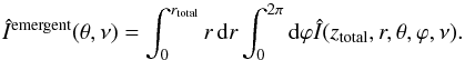 (18)We recall that, in the case of Cartesian coordinates, one performs a similar integration along x and y. It can be seen that the angular coordinate ϕ, which describes the direction where radiation plays the role of the spatial coordinate that describes the azimuth of the specific point on the disk. This is, of course, due to the axial symmetry of the medium. In practice, one needs many discrete azimuths to compute the emergent intensity in order to properly sample all line-of-sight velocities, which decreases the efficiency and time saving brought by treating this problem in a cylindrical 2D coordinate system. (Milić For a discussion of the advantages and drawbacks of numerical radiative transfer on 2D cylindrical meshes, see 2013.)
We can, however, notice that in this case the radiative transfer effects occur mostly along z and r. This means that one can compute the emergent spectrum in a rotating case by computing the emergent Stokes intensity in the static case and then performing the integration (Eq. (18)) over r and ϕ while properly red- or blueshifting the contribution of each point. That is, 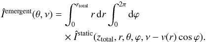 (19)This method is a mixture of exact (computation of the source function) and approximate (formal solution) approaches. (For another method that combines two different approaches, see Lamers et al. 1987.) We compared the results obtained this way with the ones computed by performing the formal solution in the rotating case using the observer’s frame formalism, and we found no significant differences. (See Appendix A for the illustration.) This means that a) Eq. (19) can be used to compute the Stokes profiles emerging from the disk, which saves time and makes the investigation of different rotation laws easier, because one only needs to perform one self-consistent NLTE solution and one formal solution in the static case, while including different rotation laws becomes a matter of post-processing; b) our assumption that lateral radiative transfer effects are negligible really does hold for this type of disk, which means that we could even attempt to emulate non-axisymmetric disks by “stitching together” pieces of different axisymmetric disks for which we have computed the emergent intensity separately. Such a computation, however, would require a detailed prior investigation because the dependence of the physical parameters (temperature, density) on the azimuth could lead to increasing the importance of lateral radiation transport.
We now inspect the emergent spectral line profiles for very simple disk models, mostly to demonstrate the effects of rotation on emergent scattering polarization profiles. All our models are isothermal, have constant opacity equal to unity and constant photon destruction probability equal to ϵ = 10-4. This is a standard value of ϵ used in academic test problems in NLTE radiative transfer computations in stellar atmosphere modeling. Constant opacity implies that the geometrical scale is identical to the optical path scale. Low value of ϵ implies that the source function is dominated by the mean intensity of the radiation field, rather than by the Planck function.
We consider four different disk models in total: they come in two different opacities and we also inspect disks which are only self-emitting as well as ones which are illuminated from the inside by a host star. The only source of radiation in the self-emitting case is the thermal energy of the gas in the disk, while in the case of illuminated disks, the main source is actually the starlight which is scattered in the disk. The radius of the star is equal to  of the disk radius and it emits like a blackbody (the star temperature is the same as the disk temperature). Note that, although the star is emitting isotropically, the disk is still illuminated anisotropically. For readers’ convenience we name these four models: A, B, Ai, Bi. We consider all four models in the static and rotating cases. The properties of the models are summed in Table 1. In the subsequent results we normalize the emergent Stokes I with respect to the area of the top surface times the Planck function, i.e. with respect to
  .
.
Disk models used to compute emergent Stokes spectra.
3.2. Self-emitting disks
 |
Fig. 3 Polarized line profiles for self-emitting cylinder of radial mean optical thickness equal to 1000 and vertical mean optical thickness equal to 10 (model A), for static (up) and rotating (down) case. Note that the rotation induces a broadening of the intensity and Q/Ic profiles, as well as non-zero Stokes U/Ic. Intensity profiles are normalized to the total emitting surface. |
Figure 3 (top panel) shows the emergent profiles for several disk inclinations (inclination of 0° indicates that the disk is viewed face-on) for the non-rotating disk. Profiles for different inclinations have similar shapes. The line center intensity decreases with increasing inclination, because we are probing regions closer and closer to the surface, where the source function is smaller. This effect is similar to limb darkening effect in stellar/solar physics. As expected, Q/Ic (we normalize the linear polarization with respect to stokes Ic at line center) increases with increasing inclination (which, again, is expected, as it is well-known from solar observations that scattering polarization rapidly increases as we observe closer and closer to the limb). Profiles again have a central “dip” due to the interplay between spatial variations of the SQ and SI source function components. We expect Stokes U to be zero, as the object is completely axisymmetric. Indeed, in our computations we find that Stokes U/Ic which is smaller than 10-5, and its (small) presence is due to slight numerical inaccuracies in the code.
From the two bottom panels of Fig. 3 it is evident that Keplerian rotation leaves a significant imprint on the emergent profiles. Firstly, profiles viewed face on remain the same, which is expected as the values of the source functions are changed negligibly, and for this viewing direction the Doppler effect has no influence as the rotation is taking place in the xy plane. With increasing inclination, the intensity profiles become broader and eventually start exhibiting double peaks and non-Gaussian shapes which are the result of the joint action of Doppler shift and inhomogeneities along z and r in the source function SI because of NLTE effects. The usual impression that disks that rotate obeying the Kepler law also exhibit a double-peaked emission is not completely true for these moderate velocities. For v0 = 10vD and high inclinations we see some indication of double peaked profile, which still has a rather interesting spectral structure.
The situation is similar when we analyze Q/Ic line profiles. They become broader, and exhibit double peaks, but, interestingly, they have approximately the same polarization in the center of the line, regardless of the rotational velocity. Their shapes are not easy to interpret as they are results of both NLTE effect, multidimensional radiative transfer effects and the presence of velocity fields. The slight “splitting” of the line can again be seen for high inclinations for the rotating case. The most interesting feature is the presence of non-zero Stokes U. It is an expected effect, already found in the paper of Vink et al. (2005) and also explained and by Smith et al. (2005) in the context of spectropolarimetric studies of active galactic nuclei. Here we discuss further on the topic and explain the origin of this polarization signature.
Firstly it is important to understand that, in the absence of large-scale magnetic fields, Q/I and U/I polarization probe the polar and azimuthal anisotropy of the radiation, respectively. In the absence of the local limb darkening/brightening (i.e. if the radiation field does not vary with θ) Stokes Q would be zero. The same stands for Stokes U in the absence of axial asymmetry. Now, note that the radiation field is, strictly speaking non-axisymmetric for any r ≠ 0. At each point in the disk, the emergent stokes U depends on (“probes”) the amount of azimuthal anisotropy.
Assume that the observer is situated on the x axis (x axis lies in the plane of the disk) and consider four elements with same radius and with azimuths equal to zero, π/ 2, π and 3π/ 2. In the absence of velocity fields, Stokes U from the first and third element would exactly cancel as well as the Stokes U signal from the second and fourth element. Now, consider the rotating disk. The radiation from the first and third element suffers no redshift and the anisotropy cancels again. However, the radiation from the element No. 2 is, for example, blueshifted while the radiation from the element No. 4 is redshifted. As a result, Stokes U profiles do not cancel but result in a double lobed profile as seen at the lower panel of Fig. 3. It slightly resembles stokes V profiles seen in solar physics and, in some distant sense it can be understood in a similar way: as a superposition of two profiles of the opposite sign, one shifted toward the blue, the other toward the red. This effect would manifest as a rotation of the plane of polarization. For this particular example, the rotation would be rather small as Stokes Q is two orders of magnitude larger than Stokes U, however, see the next section for the results for externally illuminated disks. To clarify this effect further we show a plot of Stokes U/Ic for different azimuths and given r ≈ rtotal (Fig. 4). It is clearly seen that profiles with opposite Doppler shifts have opposite signs and that they add to an antisymmetric Stokes profile. Furthermore, it is obvious that, at the very disk edge, Stokes U is rather strong (due to large axial anisotropy of the raidation) but it contributes very little to the total polarization.
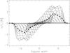 |
Fig. 4 Stokes U/Ic profiles plotted for a fixed value of r and different azimuths (thin solid lines), and resulting, azimuth integrated profile. Model A has been used for these computations. |
This effect is similar to the “optical depth effect” reported by Vink et al. (2005) for the case of continuum scattering of frequency-dependent radiation on the rotating disk. In the case of an optically thin disk (τ ≪ 1), the stokes U/Ic component is supposed to vanish. We illustrate this in Fig. 5 where we plot the emergent profiles for a rotating disk which is 100 times less opaque than model A. We plot these profiles only to show the similarity between our interpretation of the presence of the Stokes U component due to the rotation and the interpretation of Vink et al. (2005) and therefore we do not use special label for this optically thin model.
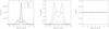 |
Fig. 5 Same as Fig. 3, but for a 100 times less opaque cylinder. For this particular case, we show only the rotating case. |
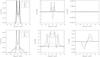 |
Fig. 6 Same as Fig. 3, but for a 10 times more opaque cylinder (Model B). Note that the presence of rotation brings a significant decrease of Stokes Q/Ic. |
Figure 6 shows the emergent profiles from the more opaque model. Intensity profiles now exhibit a deeper “dip”. This is the consequence of the fact that the near wings (i.e. “peaks”) are now formed at a depth where the source function is higher. Larger values of the source function at depth is the consequence of the much higher opacity which leads to more successful “trapping” of the photons inside the object. Q/Ic polarization in the static case shows profiles similar to the ones found by Faurobert (1988) for the case of semi-infite stellar atmosphere.
The rotating case is, not surprisingly, more complicated. The maximum intensity in Stokes I profiles decreases and they become broader, even exhibiting hints of double peaks. Although these variations in the core of the line are unlikely to be observed, due to the limited spectral resolution of todays’ instruments, broadening is an expected property of profiles formed in rotating objects. An extremely important difference between the rotating and non-rotating cases is that the profiles formed in the static medium are, without exception, emission profiles with a self-absorption “dip” in the center of the line and two peaks, corresponding to the maximum of the emission (for a detailed discussion on the location of these peaks, see Elitzur et al. 2012). Only for a very small values of vsini these dips disappear and the profiles resemble simple, one peaked, broadened (although definitely non-Gaussian) emission profile with fine variations, which are, again, likely to be smeared due to the limited spectral resolution.
Scattering polarization line profiles are even more interesting. In addition to (expected) line broadening Q/Ic also shows a significant decrease at line center. Our interpretation is that this decrease is because, on average, deeper regions of the disk are probed, due to the Doppler shift. Deeper in the medium, the anisotropy is lower, which means that one is effectively “seeing” lower value of SQ. Stokes U is again present, and increases with vrotsini, due to the same effect as in the case of optically thinner cylinders. However, the values of Stokes U in this example are lower. The explanation for this is the following: the cylinder is more optically thick along r, which leads to more isotropic radiation along the azimuth. Ultimately, this leads to lower values of SU with respect to SI and to lower signal in Stokes U/I.
To conclude this section we want to emphasize that although these models are extremely simple (homogeneous, isothermal, self-emitting), they clearly demonstrate that the combined effect of line scattering, multidimensional radiative transfer and Keplerian rotation, results not only in a change of line width, but also in a change of line shape. The emergent scattering polarization is also significantly affected. The rotation of the disk clearly results in the presence of Stokes U, which changes sign at line center. Furthermore, for disks with large optical thickness, rotational velocity also results in a decrease of Q/Ic scattering polarization, apart from the expected broadening of the line profiles. We now turn to the analysis of illuminated disk models.
3.3. Illuminated disks
Without doubt, most of gaseous disks do not radiate exclusively by themselves, at least not in the optical part of the spectrum, the band we are interested in. In some cases the disk is heated by the central body, and it emits thermal radiation so that in radiative transfer terms, we can consider it as an emitting body. In other situations, the disk is simply scattering the emergent radiation from the host object (for example a star). In this section we consider the same models as in the previous one but with with an additional internal illumination. The disks now have a “hole” equal to of the disk radial thickness, which hosts a star. We stress again that the models are very simple, homogeneous, and isothermal, with radiative transfer parameters given at the beginning of the previous section. The characteristic rotational velocity is, this time, the velocity on the inner side of the disk, which should be same as the break-up speed for the star. Apart from a Keplerian disk, we also consider one that rotates as a solid body, with angular velocity equal to the inner angular velocity of the Keplerian one. The star in the center is assumed to be spherical in shape and to emit isotropically (i.e., there is no limb darkening). The intensity of the incident radiation is identical to the value of the Planck function in the disk, that is to say, equal to unity. The total intensity of the star would in these units be around 0.1, which means that the disk and the star have approximately the same brightness.
In the subsequent results, we have not modeled any occultation effects. One occultation effect is the star occulting the disk and thus breaking the axial symmetry. The modeling of this effect is very important because it can alter the shape of the Stokes U (as is shown in, for example, Milić 2013). We chose not to include it here because we are already dealing with several different influences on the polarized line profile shape. However, we will include it in our future work, which will involve more realistic disk models. The other effect is the occultation of the star by the disk. We do not add the radiation emerging from the unocculted stellar surface to the flux. This effect cannot change the shape of the lines but can just alter the continuum level and increase the amount of unpolarized flux, thus reducing the degree of polarization of the light. We will include this effect in our upcoming work as well.
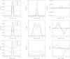 |
Fig. 7 Profiles emerging from the disk illuminated from the inside. The disk has a radial optical thickness τr = 1000 and a vertical optical thickness τz = 10 (Model Ai). Top: non-rotating disk; middle: Keplerian rotation; bottom: solid body rotation. Note that the intensity profile for the highest inclination has been scaled by a factor of 0.5. See the text for the discussion of line profile shapes. |
Figure 7 shows the emergent profile from the less opaque disk model (τz = 10, τr = 1000) for the non-rotating and rotating cases. First, note the presence of the continuum due to the transmitted light of the star in the far wings of the line. In the presence of the illuminating object, which means that the inner boundary condition for the intensity is not zero, the emitted radiation of the disk consists of three parts: i) the transmitted and attenuated light from the host star; ii) the scattered incident stellar radiation; and iii) the thermally emitted, and perhaps again scattered, radiation of the disk itself. From the first contribution, we expect an absorption line; from the other two, an emission one, because the object is not infinitely optically thick. We see, indeed, that when the inclination increases, the emission is getting weaker and weaker with respect to the transmitted continuum, and ultimately the line turns into an absorption line with some emission in the line center. Scattering polarization in Q/Ic , as expected, increases with increasing inclination and is much higher than in the previous case, predominantly because of the anisotropy introduced by the presence of the source of illumination. Stokes U is again essentially equal to zero.
The presence of rotation changes the observed profiles a lot. Stokes I is now broader and “flatter”, and we find it very possible that for specific ranges of inclinations, the line disappears since the emission and absorption contributions cancel exactly. Interestingly, the scattering polarization would remain to indicate the presence of the disk! Stokes Q/Ic is not monotonic with respect to the inclination any more because of the effect of velocity fields similar to the second example described in the previous section. The Stokes U/Ic signal is significant since the anisotropy is much higher owing to the illuminating star, and the “splitting” effect of the rotation remains, producing a double-lobed profile. This is true both for disks that rotate when obeying a Keplerian velocity law and for rigidly rotating ones. Generally, line profiles have similar shapes, but the ones emerging from the disk that rotates as a rigid body are much wider (because the velocity is constantly increasing, instead of decreasing, toward the disk edges), and subsequently, the polarization degrees are significantly lower.
It is of interest to also inspect the variation in the total line polarization P and polarization angle Θ with respect to the wavelength. (And those two quantities are also perhaps used more often in stellar physics community.) They are defined as (20)and
  (21)Figure 8 shows that the total polarization in the line for a Keperian disk changes non-monotonically with inclination. This is the effect sometimes known as the “dilution of the polarization by unpolarized radiation”: part of the original, unpolarized, flux of the star is transmitted and is effectively reducing the total polarization for high inclinations. Again, we want to stress that this is the case where we study only the radiation coming from the disk. The situation is likely to change once we properly introduce the obscuration effect by the host star (this will be done in forthcoming papers).
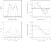 |
Fig. 8 Variation in total linear polarization P and polarization angle Θ along the line for the internally illuminated homogeneous disk with radial optical thickness equal to 1000 and horizontal optical thickness equal to 10 (Model Ai). Top: Keplerian rotation; bottom: solid body rotation. |
It is interesting that the maximum polarization angle does not change much with inclination, but the spacing between lobes does. This effect of the change in the sign of the polarization angle has been studied in more detail by Vink et al. (2005), although for the case of coherent scattering of line radiation on free electrons. It would be extremely interesting to study the differences in this effect between coherent and resonant line scattering and see if the type of scattering leaves an imprint on the variation in the polarization angle across the line. Either way, this effect could be very useful for constraining the rotational velocities of disks better. To illustrate that, we plotted the half spacing between the two rotation angle lobes versus sin i (Fig. 9). It can be seen that the dependence almost obeys a perfect linear law with a slope equal to the rotational velocity at the inner disk boundary. This means, in principle, that measurements of polarization angle in spectral lines could be used to deduce the value of v sini for circumstellar disks.
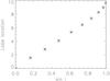 |
Fig. 9 Dependence of half-spacing between maxima of the lobes in the polarization angle line profile of the intensity for Model Ai. |
The effects are similar for disks obeying a solid body rotation, except that the total polarization, for this particular case, actually decreases with inclination. Here we obviously witness the competition between increasing scattering angle (as i approaches π/ 2, the polarization increases) and increased broadening (broader lines result in smaller maximum polarization). An interesting aspect is that, while the lobes where the polarization angles reach minimum or maximum, have approximately the same location in the Keplerian and rigidly rotating cases. In the latter we notice that the polarization angle decreases very slowly in the line wings.
To analyze the effects of optical thickness and NLTE radiative transfer further (i.e., multiple resonant line scattering), we do the computations again but for ten times more optically thick disk (Model Bi). In such a case, the radiation coming from the disk itself is non-negligible, and it mostly contributes to the intensity profiles where, for the lower three inclinations, we see a self-absorbing, emission line, superimposed on a background (transmitted) continuum (Fig. 10). The linear polarization in Stokes Q is as high as in the optically thinner case, while Stokes U is negligible, as expected.
In the presence of rotation, we see that the polarized profiles are very similar to the optically thinner disk (Fig. 7). Obviously, the polarization is formed in the region where the polarized source function is dominated by scattered radiation from the incident star. One should keep in mind that the degree of polarization only depends on the anisotropy which is obviously dominated by the anisotropic illumination of the incident radiation. This in turn results in polarized profiles that are relatively insensitive to the opacity of the disk.
Only for the low inclination case (i = 25°) do we see a drop in the degree of linear polarization both in stokes Q and U. Our interpretation is that this is due to the small scattering angle combined with the effect of multiple scatterings that destroy the polarization. For higher inclinations, on the other hand, both optically thinner and thicker disks exhibit similar polarized profiles, which is interesting. We also show the total polarization in the line and variation of the polarization angle over the line for this more opaque disk model (Fig. 11).
Also, the variation in the polarization angle across the line is very similar to the previous case (Model Ai), which is good news because it means that the potential diagnostic technique3, which relies on this, is not sensitive to the optical depth of the disk in the observed spectral line. Probably the most interesting result is that, contrary to the case of self-emitting disks, an increase in the optical thickness of the disk does not change the degree of the polarization significantly.
4. Conclusions
In this paper we have examined the effect of rotation on emergent line scattering polarization in simplified models of gaseous disks. We considered both disks that are self-emitting and ones illuminated by an inside source (i.e., star). The models are very simple: homogeneous and isothermal. The disks are also rotating according to either Keplerian or solid body rotation. To compute the emergent polarized line profiles, we used a fully consistent way of solving the equations of radiative transfer and statistical equilibrium for a two-level atom in the presence of velocity fields. We employed the so-called reduced intensity formalism, which has so far been used in solar physics but not for modeling other objects. We solved the radiative transfer equation in 2D cylindrical geometry, which is not commonly used, but for this case, it is an advantageous approach.
Even in these, perhaps unrealistic models, the parameter space to explore is fairly large: disk optical thickness, rotation velocity, size of the star with respect to the disk, ratio between disk radial and horizontal size, etc. Therefore, it is rather hard to investigate the effects of different parameters. Needless to say, in realistic models, temperature, opacity, and photon destruction probability can also vary with spatial coordinates, and rotation can deviate from the Keplerian law. That is why we have restricted ourselves in this paper to trying to demonstrate the effects of rotation on emergent polarized line profiles. We have considered rather low rotational velocities (vmax ≈ 10vD), but the presence of these even relatively weak velocity fields causes significant changes in the polarized line profiles. For internally illuminated disks, we also computed polarized profiles for disks that obey solid-body rotation to illustrate the differences between different rotational laws.
In the case of self-emitting disks, the main effects of rotation are the broadening of Stokes I and Q/Ic profiles and the presence of weak linear polarization in Stokes U/Ic. In the optically thinner case (τr = 1000, τz = 10), the Q/Ic polarization at line center does not change significantly when a rotation of the disk is introduced, while in the optically thicker case (opacity 10 times higher), the presence of rotation decreases the degree of linear polarization by about a factor of 5. The reason for this is that in our interpretation, the difference in behavior of the radiation anisotropy in the disk between the two cases. We stress once again that in neither of these cases is the disk optically thin (i.e., optical thickness along each axis is much greater than unity) or optically thick (i.e., the size of the disk along at least one axis is smaller than the photon thermalization length, 1 /ϵ). In solar/stellar atmosphere modeling it is customary to refer to such a medium as “effectively thin”, and this is exactly the case that is most interesting for radiative transfer investigations in multidimensional objects.
Internally illuminated disks show more interesting features. The presence of the anisotropic illuminating radiation makes the degree of polarization much higher. Subsequently, the “spectral splitting” between the receding (red shifted) and approaching (blue shifted) parts of the rotating disk is much more prominent in Stokes U/Ic, which now exhibits polarization degrees of a few percentage points. Talking in terms of angle of polarization ( ), this results in a significant variation in the polarization angle across the line. Interestingly, this angle does not seem to be sensitive to either the optical thickness of the disk or to the inclination (actually a combination of the rotational velocity and inclination, v sini). This means that this effect can be used for disk diagnostics, which has already been pointed out by Vink et al. (2005) and Smith et al. (2005) for the case of coherent scattering.
To conclude, here we want to emphasize that the presence of rotation strongly influences the polarized line formation process in disk-like objects. Strong influence makes room for devising intelligent diagnostic techniques, which is the goal of further research. Since spatially resolved spectropolarimetric observations of such objects are still unfeasible, one must devise diagnostic techniques that rely on spatially integrated spectropolarimetric observations. In such studies, detailed line formation modeling, such as one hinted at in this paper might prove to be necessary, and we think that techniques routinely used in solar and stellar physics should be extended to line formation in disk-like objects as well. Probably the greatest insight into the physics of these objects can be obtained by using state-of-the-art spectropolatimetric observations (ESPaDOnS, NARVAL), together with spectro-interferometric ones (CHARA, VEGA). We hope that modeling approaches, such as the ones presented in this paper, can help in the interpretation of such high-quality observations.
Our future work will present results from more realistic disk models where opacity and temperature vary inside the object and also first attempts to model observed spectral features. We also aim to introduce the so-called comoving frame formalism for the solution of radiative transfer equation in moving media, in order to be able to model rapidly rotating objects such as different kinds of accretion disks.
The rule thumb in radiative transfer is that the emergent (emerging?) radiation at frequency ν is equal to the source function at monochromatic optical depth τν. The presence of velocity fields allows one to “probe” different regions than in the static case. Because of the spatial variations of the source function this generally leads to different emergent profiles.
This diagnostic has already been presented by Smith et al. (2005), and recently used by Afanasiev et al. (2014), but for AGN disks, not circumstellar ones.
Acknowledgments
We are indebted to the anonymous referee for the detailed review, which significantly improved the quality of the manuscript. We also thank Jorick Vink, Slobodan Jankov, and Olga Atanacković for useful comments and critical reading of the manuscript. I.M. is grateful to Pavle Savić grant, COST action 1104, and the SOLARNET project for financially supporting his research and collaboration with MF. This research is also partly funded by the Serbian Ministry of Science and Education, under the project 176004, “Stellar physics”.
References
- Adam, J. 1990, A&A, 240, 541 [NASA ADS] [Google Scholar]
- Afanasiev, V. L., Popović, L. Č., Shapovalova, A. I., Borisov, N. V., & Ilić, D. 2014, MNRAS, 440, 519 [Google Scholar]
- Antonucci, R. R. J., & Miller, J. S. 1985, ApJ, 297, 621 [NASA ADS] [CrossRef] [Google Scholar]
- Anusha, L. S., & Nagendra, K. N. 2011a, ApJ, 726, 6 [NASA ADS] [CrossRef] [Google Scholar]
- Anusha, L. S., & Nagendra, K. N. 2011b, ApJ, 738, 116 [NASA ADS] [CrossRef] [Google Scholar]
- Carciofi, A. C., & Bjorkman, J. E. 2008, ApJ, 684, 1374 [NASA ADS] [CrossRef] [EDP Sciences] [Google Scholar]
- Carciofi, A. C., Okazaki, A. T., Le Bouquin, J.-B., et al. 2009, A&A, 504, 915 [NASA ADS] [CrossRef] [EDP Sciences] [Google Scholar]
- Carlsson, M. 2009, Mem. Soc. Astron. It., 80, 606 [Google Scholar]
- Dessart, L., & Hillier, D. J. 2011, MNRAS, 415, 3497 [NASA ADS] [CrossRef] [Google Scholar]
- Elitzur, M., Asensio Ramos, A., & Ceccarelli, C. 2012, MNRAS, 422, 1394 [NASA ADS] [CrossRef] [Google Scholar]
- Faurobert, M. 1988, A&A, 194, 268 [NASA ADS] [Google Scholar]
- Frisch, H. 2007, A&A, 476, 665 [NASA ADS] [CrossRef] [EDP Sciences] [Google Scholar]
- Halonen, R. J., Mackay, F. E., & Jones, C. E. 2013, ApJS, 204, 11 [NASA ADS] [CrossRef] [Google Scholar]
- Hubeny, I. 2003, in Stellar Atmosphere Modeling, eds. I. Hubeny, D. Mihalas, & K. Werner, ASP Conf. Ser., 288, 17 [Google Scholar]
- Ibgui, L., Hubeny, I., Lanz, T., & Stehlé, C. 2013, A&A, 549, A126 [NASA ADS] [CrossRef] [EDP Sciences] [Google Scholar]
- Ignace, R. 2000, A&A, 363, 1106 [NASA ADS] [Google Scholar]
- Ignace, R. 2010, ApJ, 725, 1040 [NASA ADS] [CrossRef] [Google Scholar]
- Lamers, H. J. G. L. M., Cerruti-Sola, M., & Perinotto, M. 1987, ApJ, 314, 726 [NASA ADS] [CrossRef] [Google Scholar]
- Landi Degl’Innocenti, E., & Landolfi, M. 2004, Astrophys. Space Sci. Lib., 307 [Google Scholar]
- Mihalas, D. 1978, Stellar atmospheres, 2nd edn. (San Francisco: W. H. Freeman and Co) [Google Scholar]
- Milić, I. 2013, A&A, 555, A130 [NASA ADS] [CrossRef] [EDP Sciences] [Google Scholar]
- Papkalla, R. 1995, A&A, 295, 551 [NASA ADS] [Google Scholar]
- Rivinius, T., Carciofi, A. C., & Martayan, C. 2013, A&ARv, 21, 69 [Google Scholar]
- Smith, J. E., Robinson, A., Young, S., Axon, D. J., & Corbett, E. A. 2005, MNRAS, 359, 846 [NASA ADS] [CrossRef] [Google Scholar]
- Trujillo Bueno, J. 2003, in Stellar Atmosphere Modeling, eds. I. Hubeny, D. Mihalas, & K. Werner, ASP Conf. Ser., 288, 551 [Google Scholar]
- Trujillo Bueno, J. 2009, in AIP Conf. Ser. 1171, eds. I. Hubeny, J. M. Stone, K. MacGregor, & K. Werner, 27 [Google Scholar]
- Trujillo Bueno, J., Shchukina, N., & Asensio Ramos, A. 2004, Nature, 430, 326 [Google Scholar]
- Štěpán, J., & Trujillo Bueno, J. 2013, A&A, 557, A143 [NASA ADS] [CrossRef] [EDP Sciences] [Google Scholar]
- van Noort, M., Hubeny, I., & Lanz, T. 2002, ApJ, 568, 1066 [NASA ADS] [CrossRef] [Google Scholar]
- Vink, J. S., Drew, J. E., Harries, T. J., & Oudmaijer, R. D. 2002, MNRAS, 337, 356 [NASA ADS] [CrossRef] [Google Scholar]
- Vink, J. S., Harries, T. J., & Drew, J. E. 2005, A&A, 430, 213 [NASA ADS] [CrossRef] [EDP Sciences] [Google Scholar]
- Wheelwright, H. E., Bjorkman, J. E., Oudmaijer, R. D., et al. 2012, MNRAS, 423, L11 [NASA ADS] [CrossRef] [Google Scholar]
Appendix A: Approximate calculations of the emergent Stokes profiles from a rotating disk
To further illustrate the differences (or lack thereof) between different approaches to the computation of the formal solution, we present here emergent Stokes profiles from model A computed with three different approaches:
-
1.
We compute the reduced source function in the presence of thevelocity fields and then use it to formally solve the RTE in movingmedia. This approach has no approximations and the only errorsarise from numerical inaccuracies.
-
2.
We use the source function computed in the static case and formally solve the RTE in the moving media. The formal solution here is completely consistent, while the source function is approximated to be identical to the static case.
-
3.
We use the source function computed in the static case and formally solve the RTE in the static media. We then appropriately Doppler-shift the profiles in the process of spatial (that is, angular) integration (Eq. (19)). In this approximation we assume that each “slice” of the disk behaves like a static object in terms of radiative transfer and that all changes to the spectrum arise purely because of the Doppler shift of individual disk parts (i.e., there is no lateral radiative transfer).
Emergent profiles are shown in Fig. A.1. Because the whole paper is focused on a qualitative analysis of the line shapes, we restrict ourselves to visually inspecting the differences. To justify this, we remind the reader that the current state of spectropolarimetric observations of objects outside of the solar system are fairly inaccurate (for example, see Vink et al. 2002, for some observations of Herbig Ae/Be stars) concerning the polarimetric aspect.
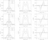 |
Fig. A.1 Comparison between polarized line profiles computed from the Model A in the presence of Keplerian rotation using approaches 1 (upper panel), 2 (middle panel), and 3 (lower panel) described in the Appendix. |
The notable difference is the presence of a very weak Stokes U in the far wings on the line that can be seen only when the approach 1 is used. However, since this effect is more than an order of magnitude weaker than the maximum polarization in Stokes U, we feel that the difference from two other cases is negligible. In the top two plots also a slight asymmetry in Stokes Q/Ic can be seen. This is the effect of an insufficient number of points in φ, which results in numerical inaccuracies. As is stated in the text, the integration over the azimuth is actually the spatial integration, because we assume that the disk is axisymmetric. For computations by approaches 1 and 2, we have used 36 Gaussian points in azimuth and 121 equally spaced points in frequency. The major advantage of the third approach is that the number of frequency points can be significantly smaller because there is no need to cover all possible red/blue shifts in the frequency mesh.
All Tables
All Figures
|
Fig. 1 2D distribution of SI source function in the z,r plane for the non-rotating cylinder (up) and relative difference between rotating and static case (down). The source function is given in units of the Planck function. Both z and r axis are double-logarithmic; i.e., the sampling is finer toward the disk boundaries. |
| In the text | |
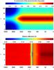 |
Fig. 2 Same as in Fig. 1, but for a ten times more opaque cylinder. |
| In the text | |
|
Fig. 3 Polarized line profiles for self-emitting cylinder of radial mean optical thickness equal to 1000 and vertical mean optical thickness equal to 10 (model A), for static (up) and rotating (down) case. Note that the rotation induces a broadening of the intensity and Q/Ic profiles, as well as non-zero Stokes U/Ic. Intensity profiles are normalized to the total emitting surface. |
| In the text | |
|
Fig. 4 Stokes U/Ic profiles plotted for a fixed value of r and different azimuths (thin solid lines), and resulting, azimuth integrated profile. Model A has been used for these computations. |
| In the text | |
|
Fig. 5 Same as Fig. 3, but for a 100 times less opaque cylinder. For this particular case, we show only the rotating case. |
| In the text | |
|
Fig. 6 Same as Fig. 3, but for a 10 times more opaque cylinder (Model B). Note that the presence of rotation brings a significant decrease of Stokes Q/Ic. |
| In the text | |
|
Fig. 7 Profiles emerging from the disk illuminated from the inside. The disk has a radial optical thickness τr = 1000 and a vertical optical thickness τz = 10 (Model Ai). Top: non-rotating disk; middle: Keplerian rotation; bottom: solid body rotation. Note that the intensity profile for the highest inclination has been scaled by a factor of 0.5. See the text for the discussion of line profile shapes. |
| In the text | |
|
Fig. 8 Variation in total linear polarization P and polarization angle Θ along the line for the internally illuminated homogeneous disk with radial optical thickness equal to 1000 and horizontal optical thickness equal to 10 (Model Ai). Top: Keplerian rotation; bottom: solid body rotation. |
| In the text | |
|
Fig. 9 Dependence of half-spacing between maxima of the lobes in the polarization angle line profile of the intensity for Model Ai. |
| In the text | |
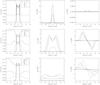 |
Fig. 10 Same as Fig. 7, but for a 10 times more opaque disk (Model Bi). |
| In the text | |
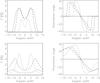 |
Fig. 11 Same as Fig. 8 but for a 10 times more opaque disk (Model Bi). |
| In the text | |
|
Fig. A.1 Comparison between polarized line profiles computed from the Model A in the presence of Keplerian rotation using approaches 1 (upper panel), 2 (middle panel), and 3 (lower panel) described in the Appendix. |
| In the text | |
Current usage metrics show cumulative count of Article Views (full-text article views including HTML views, PDF and ePub downloads, according to the available data) and Abstracts Views on Vision4Press platform.
Data correspond to usage on the plateform after 2015. The current usage metrics is available 48-96 hours after online publication and is updated daily on week days.
Initial download of the metrics may take a while.