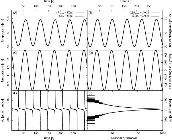
Results of a simulation which shows how φ_D is computed. We assume to observe a 1 K peak-to-peak dipole in the sky for 5 minutes with a scanning strategy very similar to the one used for Planck’s 30 GHz radiometers, i.e., the sky is scanned in circles of high amplitude (~85°) with a rotation frequency ν = 1 / 60 Hz and a sampling frequency of 32.5 Hz (so that 10 000 temperature samples are generated for each data stream). We observe the dipole using a realistic 30 GHz beam B = B_main + B_side with FWHM . Panel A): plot of the (B_main ∗ D)(t) term, which oscillates as a sinusoid with amplitude ≲ 0.5 K; the term (B_sl ∗ D)(t) is negligible (see panel C for a close-up). Panel B): plot of the ∂_t(B_main ∗ D)(t) term, used in the definition of φ_D (Eq. (9)). Panel C): Close-up of the (B_sl ∗ D)(t) term shown in panel A). Panel D): close-up of the ∂_t(B_sl ∗ D)(t) shown in panel B). Panel E): value of φ_D as a function of time, calculated using the definition in Eq. 9. Panel F): distribution of the 10 000 values of φ_D plotted in panel E). Half of the values fall within the 0.19–0.34% range.