| Issue |
A&A
Volume 570, October 2014
|
|
|---|---|---|
| Article Number | A73 | |
| Number of page(s) | 11 | |
| Section | Extragalactic astronomy | |
| DOI | https://doi.org/10.1051/0004-6361/201424662 | |
| Published online | 21 October 2014 | |
Multiwavelength campaign on Mrk 509
XIV. Chandra HETGS spectra
1
SRON Netherlands Institute for Space Research, Sorbonnelaan 2, 3584 CA
Utrecht, The
Netherlands
e-mail: This email address is being protected from spambots. You need JavaScript enabled to view it.
2
Department of Physics and Astronomy, Universiteit
Utrecht, PO Box
80000, 3508 TA
Utrecht, The
Netherlands
3
Leiden Observatory, Leiden University,
PO Box 9513,
2300 RA
Leiden, The
Netherlands
4
European Space Astronomy Centre (ESAC),
PO Box 78, 28691
Villanueva de la Cañada,
Madrid,
Spain
5
Department of Physics, Virginia Tech, Blacksburg, VA
24061,
USA
6
Department of Physics, Technion-Israel Institute of
Technology, 32000
Haifa,
Israel
7
Dipartimento di Matematica e Fisica, Università degli Studi Roma
Tre, Via della Vasca Navale
84, 00146
Roma,
Italy
8
Mullard Space Science Laboratory, University College
London, Holmbury St. Mary,
Dorking, Surrey,
RH5 6NT,
UK
9
INAF-IASF Bologna, Via Gobetti 101, 40129
Bologna,
Italy
10
Space Telescope Science Institute, 3700 San Martin Drive, Baltimore, MD
21218,
USA
11
Department of Physics and Astronomy, The Johns Hopkins
University, Baltimore, MD
21218,
USA
12
Max Planck Institut für Extraterrestrische Physik ,
85741
Garching,
Germany
13
University of Geneva, 16, ch. d’Ecogia, 1290
Versoix,
Switzerland
14
Univ. Grenoble Alpes, IPAG, 38000
Grenoble,
France
15
CNRS, IPAG, 38000
Grenoble,
France
16
Institute of Astronomy, University of Cambridge,
Madingley Road, Cambridge
CB3 0HA,
UK
17
Instituto de Astronomía, Universidad Católica del
Norte, Avenida Angamos 0610,
Casilla
1280
Antofagasta,
Chile
18
Department of Physics, University of Oxford,
Keble Road, Oxford
OX1 3RH,
UK
Received: 23 July 2014
Accepted: 29 August 2014
Abstract
Context. We present in this paper the results of a 270 ks Chandra HETGS observation in the context of a large multiwavelength campaign on the Seyfert galaxy Mrk 509.
Aims. The HETGS spectrum allows us to study the high ionisation warm absorber and the Fe-K complex in Mrk 509. We search for variability in the spectral properties of the source with respect to previous observations in this campaign, as well as for evidence of ultra-fast outflow signatures.
Methods. The Chandra HETGS X-ray spectrum of Mrk 509 was analysed using the SPEX fitting package.
Results. We confirm the basic structure of the warm absorber found in the 600 ks XMM-Newton RGS observation observed three years earlier, consisting of five distinct ionisation components in a multikinematic regime. We find little or no variability in the physical properties of the different warm absorber phases with respect to previous observations in this campaign, except for component D2 which has a higher column density at the expense of component C2 at the same outflow velocity (−240 km s-1). Contrary to prior reports we find no −700 km s-1 outflow component. The O viii absorption line profiles show an average covering factor of 0.81±0.08 for outflow velocities faster than −100 km s-1, similar to those measured in the UV. This supports the idea of a patchy wind. The relative metal abundances in the outflow are close to proto-solar. The narrow component of the Fe Kα emission line shows no changes with respect to previous observations which confirms its origin in distant matter. The narrow line has a red wing that can be interpreted to be a weak relativistic emission line. We find no significant evidence of ultra-fast outflows in our new spectrum down to the sensitivity limit of our data.
Key words: galaxies: active / quasars: absorption lines / X-rays: general / X-rays: galaxies / galaxies: individual: Mrk 509
© ESO, 2014
1. Introduction
Active galactic nuclei (AGN) are powered by gravitational accretion of matter onto a central supermassive black hole. It is thought that the intense radiation field might be powerful enough to drive gas outflows from the nucleus. The widespread occurrence of these outflows was recognised after the development of high-resolution UV and X-ray spectrographs, which were able to identify their signatures in the form of absorption lines of a photoionised gas, the so-called warm absorber (WA), blueshifted with respect to the rest frame of the source (Crenshaw et al. 1999; Kaastra et al. 2000). An extensive overview of these outflows can be found in Crenshaw et al. (2003).
Despite their importance, several questions regarding the origin, geometry, and structure of the WA remain open. The proposed origins for AGN outflows are disc-driven winds (Elvis 2000) and thermally driven winds emanating from the putative dusty torus (Krolik & Kriss 2001). The discovery of blueshifted Fe K-shell lines in radio-quiet AGN (e.g. Chartas et al. 2002, 2003) were interpreted with the so-called ultra-fast outflows, defined as highly ionised winds (log ξ ~ 3−6) outflowing at velocities faster than −10 000 km s-1 (Tombesi et al. 2010). In this context, it has been proposed that the ultra-fast outflows are launched as a disc wind, close to the central black hole, whereas WA are launched farther out, thus forming a stratified wind (Kazanas et al. 2012; Tombesi et al. 2013).
Here we present the results of a 270 ks Chandra HETGS observation of the Seyfert 1 galaxy Mrk 509 in the context of a large multiwavelength campaign. Mrk 509 is one of the brightest Seyfert galaxies in the sky (L (1−1000 Ryd) = 3.2 × 1038 W), and it is considered one of the closest (z = 0.034397) Seyfert 1/QSO hybrids. Because of its brightness and confirmed presence of UV and X-ray absorbers, Mrk 509 was the subject of an extensive multiwavelength campaign in 2009 described in Kaastra et al. (2011b). The present Chandra data were taken in 2012.
This paper is organised as follows. In Sect. 2 we describe the data reduction. In Sect. 3 we analyse the spectral lines, while in Sect. 4 we study the O viii line profile. The overall modelling of the outflow and the Fe-K complex are described in Sect. 5 and Sect. 6, respectively. In Sect. 7 we search for ultra-fast outflows in our spectrum. In Sect. 8 we discuss our results and, finally, we report our conclusions in Sect. 9.
Throughout the paper, the C-statistics fitting method is used, and the quoted errors refer to 68.3% confidence level (ΔC = 1 for one parameter of interest) unless otherwise stated.
2. Data reduction
Mrk 509 was observed by Chandra with the HETGS between 4 and 9 September 2012. The Chandra observation was split into two parts, separated by 19 h: observation nrs. 13864 and 13865, with exposure times of 170 and 99 ks, respectively. The data were analysed using the standard CIAO version 4.4 tools.
The spectra and response matrices were converted into SPEX (Kaastra et al. 1996) format, and that package was used for all spectral analysis. The standard High Energy Grating (HEG) and Medium Energy Grating (MEG) spectra are slightly-oversampled hence we binned them by a factor of 2 to about 1/3–1/2 of the full width at half maximum (FWHM) of the respective gratings.
2.1. Spectral modelling
It appears that when the fluxed MEG and HEG spectra are plotted, the HEG/MEG flux ratio is fairly constant at an average value of 0.954 ± 0.004 in the 3–13 Å band. In the lower wavelength band, between 1.5–3 Å, this ratio is rising with an average value of 0.999 ± 0.016. At the other side of the spectrum, between 13–16 Å, the HEG/MEG flux ratio is lower, on average 0.90 ± 0.05. For these reasons we restricted the data range to 2.5−26 Å for MEG (at the long wavelength end the statistics becomes too poor), and to 1.55–15.5 Å for HEG. In our combined spectral fits we rescaled the response matrix of the HEG uniformly by a factor of 0.954 to get consistent spectra for HEG and MEG over the relevant wavelength range.
2.2. Time variability
We checked variability of the source by constructing the zeroth order lightcurve using 1000 s bins. For the first observation, the average count rate was constant at a value of 0.3351 ± 0.0014 counts/s. We find strict upper limits to any linear flux changes; they correspond to flux differences compared to the mean flux of less than 0.7%. Interestingly, the second observation has the same average count rate within the error bars, 0.3343 ± 0.0018 counts/s. However, this observation shows a weak declining trend, with an almost linear flux decrease of 4.6 ± 1.9% between the start and the end of the observation. Compared to the XMM-Newton observations 3 years earlier, the variability on these short timescales is remarkably low. For this reason we have combined both observations and only consider the single time-averaged HETGS spectrum.
Apart from the flux constancy during the Chandra observations in 2012, also the fluxed continuum spectrum of the Chandra observation over the 5–25 Å range agrees within 5% with the fluxed RGS spectrum taken in 2009. The similarity is even stronger: we have measured the equivalent width of the seven strongest absorption lines in common between the RGS and HETGS spectra, and found that they are the same within the error bars. The HST/COS UV band also shows no strong differences in flux between the 2009 and 2012 observations (less than 5% at 1360 Å). Given this similarity of the spectra, we will adopt for our modelling the same ionising spectral energy distribution (SED) as used for the analysis of the XMM-Newton data of 2009 (Kaastra et al. 2011b; Detmers et al. 2011).
2.3. Velocity scale
The proper wavelength calibration for the RGS spectra of Mrk 509 was rather complex, see Kaastra et al. (2011a). This is essentially due to the lack of a zeroth-order spectrum in the RGS. Because of small non-linearities in the HRC-S detector used with the Chandra LETGS spectra in 2009 there remains some uncertainty in the wavelength scale, estimated by Kaastra et al. (2011a) to be about 1.8 mÅ, corresponding to about 30 km s-1.
For the HETGS the situation is more straightforward because of the presence of the zeroth-order combined with the extremely linear wavelength scale provided by the solid state ACIS-S detector chips. We have corrected our standard extracted HETGS spectra only for the Doppler motion of the Earth around the Sun, which was 12.7 km s-1 towards Mrk 509.
We have measured the outflow velocities derived from the 7 strongest absorption lines in common between the HETGS and the RGS spectra (Ne ix and Ne x 1s–2p; O vii 1s–2p, 1s–3p and 1s–4p, and O viii 1s–2p and 1s–3p). There is a perfect linear correlation between both velocity scales. Adopting the HETGS velocity scale to be correct, the velocities derived from the RGS spectra in Kaastra et al. (2011a) and subsequent papers need to be increased by + 55 ± 21 km s-1 (i.e. they are less blueshifted). This correction is just about twice the uncertainty of 30 km s-1 that was derived before on this for the RGS velocity scale.
From the above analysis we have excluded one line, namely the Mg xi 1s–2p line. The RGS spectrum (Kaastra et al. 2011a) showed a clear line (> 5σ significance) at a velocity of −545 ± 150 km s-1, corrected to the HETGS scale. However, for the same Mg xi transition the HETGS spectrum has a velocity of −200 ± 60 km s-1. We discuss this in Sect. 8. From now onwards we will report all velocities from the RGS analysis, including those reported by Detmers et al. (2011), corrected to the HETGS scale.
3. Analysis of spectral lines
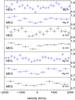 |
Fig. 1 Normalised line profiles for Si and Mg lines. Line identifications and gratings are indicated in the panels. The dotted lines correspond to the expected line profile for an infinitely narrow absorption line at outflow velocity 0 convolved with the instrumental line-spread function and with a depth corresponding to the depth of the observed spectral line. They serve to show the typical instrumental broadening. |
We have determined line profiles for the stronger spectral lines as follows. Over small wavelength ranges, the spectrum expressed in photons m-2 s-1 Å-1 is rather flat. Therefore, we determined the average continuum flux level for each line in a band between 10 000 and 20 000 km s-1 offset at each side of the line. From this continuum range we exclude the narrow absorption lines as well as the weak broad emission lines associated with some of these lines (Detmers et al. 2011). The spectra near the lines were normalised to this level and are shown in Figs. 1 and 2.
It is seen that all lines are significantly broader than the spectral resolution of the instrument, and most of them show a blue wing extending up to several hundred km s-1, a clear signature of outflow. Several spectral lines show almost black line cores, indicative for a high optical depth, in particular the Ne x and O viii 1s–2p transitions. This last line even shows some evidence of a red wing, and in its blue wing extends up to −600 km s-1 or even up to −1200 km s-1 (Fig. 2). Interestingly, while the line is very deep, it appears not to be completely black. A similar behaviour appears to be the case for the O vii 1s–2p line, although because of the strong drop of sensitivity of the MEG towards long wavelengths the significance is somewhat lower than for O viii.
Because for O viii both the 1s–2p and 1s–3p lines are well-resolved and have a good statistical quality, we first perform a detailed analysis of the line profiles of both lines.
4. Velocity-resolved line spectroscopy of O viii
In the UV-band, thanks to the high-resolution of instruments like FUSE, STIS and COS, it has been possible to do velocity-resolved line spectroscopy on sets of lines from the same ion in order to derive covering factors and column densities as a function of outflow velocity (e.g. Arav et al. 2002). In the X-ray band this has been harder to do because of the lower spectral resolution and smaller number of photons. Mrk 509 is one of the brightest Seyferts on the sky, however, and our deep exposure with the HETGS provides us with a suitable pair of lines from O viii: the 1s–2p (Lyα) and 1s–3p (Lyβ) lines (Fig. 2). The 1s–2p line is several times broader than the spectral resolution of the MEG grating.
We have modelled the velocity-dependent transmission T(ν) of both components as
follows: 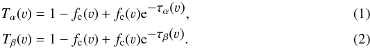 Here τβ(ν) =
(λβfβ/λαfα)
τα(ν) with fα and fβ the oscillator strengths
of both lines (actually doublets) and λα and λβ their wavelengths.
Furthermore, fc(ν) is the velocity-dependent covering
factor.
Here τβ(ν) =
(λβfβ/λαfα)
τα(ν) with fα and fβ the oscillator strengths
of both lines (actually doublets) and λα and λβ their wavelengths.
Furthermore, fc(ν) is the velocity-dependent covering
factor.
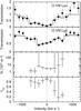 |
Fig. 3 Velocity-dependent total O viii column density N and covering factor fc (lower panels) deduced from fits (upper two panels) to the O viii Lyα and Lyβ lines. |
We show our results in Fig. 3. Only the portions of the profile with well-determined covering factor or column density are shown. Between −700 and + 200 km s-1 the covering factor is fairly constant with a mean value of 0.86 ± 0.05, because over this velocity range the Lyα line is deep but not completely black. While the continuum near this line has about 15 counts/bin, the line core has 15 net counts distributed over 6 bins (the subtracted background is negligible).
The covering factor for the red wing of the line (between + 200 and + 700 km s-1) appears to be lower, on average about 0.31 ± 0.10.
We have ignored here the contribution from any underlying broad emission line. If we add the contribution from an emission line with a width (4200 km s-1 FWHM) and strength (peak flux 6.7% of the continuum) equal to that derived by Detmers et al. (2011) for the RGS-spectrum of Mrk 509, and assume that the covering factor for the line is equal to that for the continuum, the average covering factor in the region below and above + 200 km s-1 increases to 0.87 ± 0.09 and 0.32 ± 0.16, respectively. This is only a modest difference.
5. Detailed spectral modelling of the outflow
A detailed analysis of line profiles is only possible for the stronger lines (see the previous section). Full spectral fitting is needed to make use of the information contained in all absorption lines, including the weaker lines. Such an analysis was done using the RGS spectrum (Detmers et al. 2011). Because the HETGS has 3−6 times higher spectral resolution than the RGS, and the line profiles of some lines (for instance O viii 1s−2p) seem to indicate the presence of outflow components with higher velocity than considered by Detmers et al. (2011), we repeat their analysis but taking into account also the HETGS data.
5.1. Choice of velocity components
The spectral resolution of the HETGS is significantly better than that of the RGS, but still we lack the velocity resolution that is available in the UV. Taking too many not fully independent velocity components in a spectral model leads to strong correlations between these components and a poorly defined solution. It is therefore necessary to limit the number of velocity components taking into account the instrumental resolution. The FWHM of the MEG for the strongest lines (O viii) is about 300 km s-1. For the HEG we get a similar FWHM but now for the shorter wavelength lines like Ne x and Mg xii. Ideally, a velocity bin size of about 1/3 FWHM would be achievable, but given the limits imposed by the statistics of the spectrum (relatively low effective area in the oxygen region), a minimum bin size of about 150−200 km s-1 seems appropriate.
The lowest velocity gas found by Detmers et al. (2011) is component B1, with a corrected velocity of + 80 ± 30 km s-1. This component agrees fairly well in velocity, column density and ionisation parameter with the UV troughs T5–T7 defined by Arav et al. (2012), with centroid velocities at −15, + 45 and + 125 km s-1, respectively. The column-density weighted average velocity of these UV components is about +50 km s-1, and we will adopt that velocity as one of our basic components. From Fig. 2 we see that there is some material at such velocities for lines with ionisation parameter log ξ less than about 2.0 (O viii).
The UV data show a lack of material with velocities between about −200 and −100 km s-1. The highest velocities measured in the UV are from the troughs T1 (−405 km s-1), T2 (−310 km s-1), and T3 (−240 km s-1). From our individual line analysis, we find that the line centroid of the lines from the ions that are dominated by ionisation component D in the notation of Detmers et al. (2011) (Si xiv, Si xiii, Mg xii and Ne x) have a weighted average outflow velocity of −227 ± 24 km s-1, consistent with the velocity of UV trough T3. Hence, we will also adopt a velocity of −240 km s-1 as one of our basic components.
The third velocity component then naturally corresponds to trough T1 at −405 km s-1. Given the resolution of the HETGS, we will not be able to fully disentangle the troughs T1–T3, but by choosing T1 and T3 as our base components we will be able to model the X-ray velocity structure with sufficient accuracy. Any gas present at the velocities of T2 will be partly assigned to T1 and partly to T3.
Finally, Detmers et al. (2011) found some evidence of higher velocity gas at around −700 km s-1, mainly in the Mg xi and Fe xx and Fe xxi ions. Our line profile for Mg xii (Fig. 1) seems to exclude such a component, although the broad blue wing of O viii might be consistent with such a component. Therefore we will include a fourth velocity component labelled T0 at −700 km s-1.
We summarise our adopted components in Table 1 below.
Adopted velocity components for the analysis of the HETGS spectrum.
5.2. Spectral modelling
We have first made a simultaneous fit to the RGS and HETGS data. The continuum model that we used is a small modification of the model used by Detmers et al. (2011). While they used a pure spline for the full continuum of the RGS spectrum, we use the sum of a power-law component and a spline. The power-law gives a fair description of the high-energy part of the HETGS spectrum (apart from Fe-K line features). While Detmers et al. (2011) used the spline to describe the full continuum (power-law plus soft excess), now it describes only the soft excess component. For the RGS, the spline has 12 knots, logarithmically spaced between 5–40 Å, with the flux value at 5 Å forced to be zero, such that for λ< 5 Å the continuum is given by the power-law. For the HETGS spectrum, we use a linear wavelength grid for the spline, with a spacing of 2 Å between 6.5−26.5 Å, and again with zero flux at λ = 6.5 Å. In our spectral fitting, the splines representing the soft excess are allowed to vary independently for both datasets to account for weak time variability and cross-calibration effects, both of which are most important at lower energies where both instruments overlap. We keep the photon index of the power-law frozen to a value determined from a preliminary fit to the HETGS data. Because the RGS does not cover the λ< 5 Å regime, the precise value of the photon index is not important for RGS; any differences with the “true” underlying power-law in the soft band are compensated for by the spline.
Furthermore, we add three broad Gaussian emission lines for the 1s–2p transitions significantly detected in the RGS spectrum: O viii, O vii and Ne ix, with their width frozen to the value obtained by Detmers et al. (2011) for the RGS spectrum (FWHM 4200 km s-1). The line fluxes are also frozen to the values obtained from the RGS spectrum.
The foreground Galactic absorption model is also the same as used by Detmers et al. (2011) and described in more detail by Pinto et al. (2012).
We next add photo-ionised absorption components (the xabs model of SPEX). This model describes the transmission of a thin layer of photo-ionised gas.
We first start testing how many absorption components are needed. For that purpose, we incorporate a total number of 7 × 4 = 28xabs components in our model. For each of the 4 velocity components, we use 7 different ionisation components, with values of log ξ frozen to 0, 0.5, 1, 1.5, 2, 2.5 and 3, respectively. For this spacing of ionisation parameter, any gas with ionisation parameter in the range of log ξ between 0−3 will give a detectable signal for at least 1 component. In addition, as discussed before our spacing of the velocity components is sufficient to include all gas. The velocity broadening was fixed to σv = 100 km s-1 for each component. Only the column densities of all 28 components are free parameters. This is sufficient for the present purpose, namely to detect all relevant spectral components.
Figure 4 shows the result of a joint fit to the RGS and HETGS spectrum. At the lowest velocity (+50 km s-1) we find two components, close to components B1 and C1 defined by Detmers et al. (2011). For gas at −240 km s-1 a blend of the components C2 and D2 is recovered: it should be noted that in the analysis of Detmers et al. (2011) the ionisation parameters and outflow velocities were free parameters, giving more flexibility than in the present analysis with fixed ionisation parameters. Component A2 is also recovered at this velocity. Finally, at −405 km s-1 we find gas at log ξ = 3, corresponding to component E2. For this highest ionised component, there is a strong correlation between column density and ionisation parameter such that the 1σ lower limit for component E2 (not shown in the figure) is closer to our component at log ξ = 3 both in ionisation parameter and column density.
It thus appears that there is little room for more absorption components than the ones already found by Detmers et al. (2011). However, to test this in more detail, we have also investigated another model.
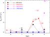 |
Fig. 4 Best-fit column densities for a model with 28 absorption components applied to the joint RGS and HETGS spectra. Crosses with labels indicate the positions of the components found in the analysis of the RGS spectrum by Detmers et al. (2011). |
We use a model with 8 xabs components, but contrary to our analysis above we allow three main parameters (log ξ, NH, and the velocity dispersion σv) to be free. The outflow velocities are frozen to one of the values from Table 1. For six of these components, we use initial conditions close to the values for components A2, B1, C1, C2, D2 and E2 of Detmers et al. (2011). To test whether there is gas present at log ξ> 3 we added a seventh component with a velocity of −405 km s-1 and a high ionisation parameter. The HETGS, because of its wavelength range, is well suited to detect highly ionised absorption. For component 8 we use an outflow velocity of −700 km s-1 with an initial ionisation parameter in the range where O viii has its peak concentration, in order to see if we can confirm the blue wing of the O viii line (Fig. 2). We execute the spectral fits three times: for the RGS only, HETGS only and for the combined RGS and HETGS spectrum.
Parameters of the spectral fits with multiple ionisation components
The best-fit parameters are shown in Table 2. We first consider the already known components B1–E2. In general, the statistical uncertainties on the HETGS spectrum are somewhat larger than on the RGS spectrum. This is caused by the factor of two difference in exposure time and the larger effective area at longer wavelengths, both in favour of the RGS. Interestingly, the only significant variability appears to occur for component C2 (4.2σ significance decrease) and D2, with a tripling of the column density (2.8σ significance).
The additional two components are poorly constrained. The column density of the component at −405 km s-1 must be regarded as an upper limit. The component at −700 km s-1 also converged to a high-ionisation value, with low significance and poor constraints. Again, the column density is merely an upper limit.
5.3. Abundances
Best-fit abundances in the outflow of Mrk 509 relative to oxygen and in proto-solar units.
Using our model with the six significant xabs components presented in the previous section we have also determined the abundances in the outflow by making them free parameters. As discussed in Steenbrugge et al. (2011), we keep the oxygen abundance frozen to the proto-solar value (Lodders & Palme 2009), because the X-ray spectrum contains no hydrogen or helium lines. Thus, all abundances are relative to oxygen. We determined the abundances using both the combined RGS and HETGS spectrum as well as using only the HETGS spectrum. We show our results in Table 3. The abundances of the combined fit are not always strictly between those derived from the individual RGS and HETGS fits. This is caused by the different bandpass of both instruments and the slightly different spectral models, but in general the abundances agree within their nominal statistical uncertainties.
5.4. The 2–6 keV band
Our HETGS spectrum has the best combination of sensitivity with spectral energy resolution over the 2–6 keV band. We have searched for the presence of absorption and emission lines in this band, but there are no features stronger than our detection limit of about 3 mÅ equivalent width in this band. This is consistent with the prediction from our model for the outflow presented before in this section. The same model also predicts that the lines from innershell absorption lines in the Fe-K band are below the detection limit of the HETGS data. Limits for ultra-fast outflows in this band are discussed in Sect. 7.2.
6. The Fe-K complex
6.1. General considerations
Our present HETGS spectrum is the best-exposed high-resolution spectrum of Mrk 509 in the Fe-K band. Yaqoob & Padmanabhan (2004) detected a narrow iron line in a shorter, 59 ks HETGS spectrum taken in 2001. The analysis of the XMM-Newton pn spectrum (Ponti et al. 2013) shows that the neutral Fe-K emission line has two components: a narrow component that remains constant in flux over time, and a broader component with a constant equivalent width from days to years timescales. In addition, the XMM-Newton spectrum shows excess flux between 6.7–7.0 keV that can be modelled well with two different models: a weak relativistically broadened emission line or weak highly-ionised line emission from H-like or He-like iron, possibly produced by scattering from distant material.
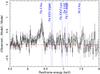 |
Fig. 5 HEG spectrum near the Fe-K emission line. Shown are the residuals relative to a power-law continuum. The rest frame energies of some important transitions are indicated by dotted lines (the Fe xxv Lyα line consist of two components, and the Fe xxv triplet consists of four components, from left to right the forbidden line, the intercombination lines and the resonance line). |
Our HEG spectrum near the Fe-K complex is shown in Fig. 5. The spectrum is shown relative to the power-law continuum obtained from the model fit discussed below (Fig. 6). The most obvious feature in the spectrum is the narrow emission line at 6.4 keV rest frame energy which shows a red shoulder extending down to 6.25 keV, and perhaps even down to about 5.8 keV. We treat these features in more detail in Sect. 6.2 below. Because of the statistical uncertainties of the spectrum, we cannot prove the presence of other spectral features at higher energies, although, for instance, the residuals in Fig. 5 near the Fe xxv and Fe xxvi 1s−2p transitions are consistent with the predictions from the XMM-Newton model of Ponti et al. (2013) (equivalent width about 4 eV for each line).
Ponti et al. (2013) described the 6.4 keV line by the sum of a narrow and broad (σ = 0.22 keV) Gaussian line. Our data are still consistent with such a model and the strengths of the lines derived by Ponti et al. (2013), but this model cannot reproduce the strong red wing of the narrow line, unless the broad line would be four times stronger and would lack a blue wing. Therefore we model this spectral region with a different model as outlined in the next section.
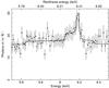 |
Fig. 6 HEG spectrum in 2012 near the Fe-K emission line (data points with error bars). The model (solid line) consists of a power-law, narrow emission line and two flat plateaus. |
6.2. Analysis of the Fe-K emission line
The spectrum near the narrow line at 6.4 keV rest frame energy is shown in Fig. 6. In addition to the narrow line, there is a broad red wing extending down to 6.25 keV, and perhaps even down to about 5.8 keV.
We have fitted the continuum first using the continuum model described in Sect. 5.2, i.e. a high-energy powerlaw and a spline at low energies representing the soft excess. We added the outflow as modelled by the sum of xabs components but with their parameters frozen to the values found in Sect. 5.2. Only the parameters of the power-law and the spline were allowed to vary.
We then added a narrow iron line at 6.40 keV to the model (assumed to be a δ-line). The red wing of the line extending down to ~6.25 keV could suggest perhaps the presence of a Compton shoulder. In order to test this, we have added a flat plateau to the model. It consists of a δ-line with centre 6.336 keV, smeared with a flat profile (the vblo component of SPEX) with a full-width of 0.15 keV. This mimics to lowest order the Compton shoulder profiles as presented e.g. by Matt (2002). The even broader red wing is modelled here with a similar flat profile with centre 6.2 keV and half-width of 0.73 keV.
We obtain a best fit normalisation of the narrow line of 0.09 ± 0.03 ph m-2 s-1 or an equivalent width of 16 ± 5 eV. For the narrow plateau we obtain a flux of 0.19 ± 0.06 ph m-2 s-1 or an equivalent width of 33 ± 10 eV. The broadest plateau has a flux of 0.41 ± 0.10 ph m-2 s-1. Without the broadest plateau in the model, the narrow line would have a slightly higher flux of 0.10 ph m-2 s-1 and its red wing a flux of 0.28 ph m-2 s-1. See Fig. 6 for this empirical fit.
As an alternative model, we have used the same model but with the two plateau components replaced by a relativistically blurred emission line. For that purpose we use the refl model of SPEX, which was provided by Piotr Zycki. It calculates the reflected continuum plus the corresponding Fe-K line from a constant density X-ray illuminated atmosphere. It computes the Compton-reflected continuum (cf. Magdziarz & Zdziarski 1995) and the iron Kα line (cf. Zycki & Czerny 1994), as described in Zycki et al. (1999). In addition it can be convolved with a relativistic discline model (for Schwarzschild geometry).
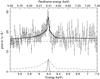 |
Fig. 7 HEG spectrum near the Fe-K emission line (data points with error bars) fitted to a model with a narrow emission line and a relativistically blurred cold reflection component. The lines are from bottom to top: contribution from the narrow emission line (solid), reflection component (dot-dashed), powerlaw component (dashed), sum of power law and reflection (dotted) and total model (solid histogram). |
Model for the Fe-K emission line region.
This model gives an acceptable solution, but because the corresponding line is not very strong, we have kept a few parameters fixed. We kept the inner- and outer disc radius frozen to 6 and 104 gravitational radii, the metallicity and iron abundance to solar values and the ionisation parameter to zero (i.e. cold reflection). We show our solution in Table 4 and Fig. 7.
7. Ultra-fast outflows
7.1. Fe-K region
Ultra-fast outflows (e.g. Tombesi et al. 2010) have been previously reported for Mrk 509. Dadina et al. (2005) report a redshifted system (+0.21c if interpreted as Fe xxvi) in two out of five time segments of one of the six BeppoSAX observations taken between 1998–2001, as well as a blue-shifted system at −0.16c in one of these time segments. In addition, they report an outflow system at −0.19c in the XMM-Newton observation taken in 2000. Cappi et al. (2009) reported three systems in three different XMM-Newton observations taken in 2000, 2005 and 2006. They have equivalent widths of 32 ± 12, 20 ± 6 and 20 ± 7 eV at outflow velocities of −0.172c, −0.141c and −0.196c, respectively, when identified with Fe xxvi 1s–2p. In the stacked XMM-Newton data taken before 2009, Ponti et al. (2009) found evidence of an additional system with an outflow velocity of −0.048c and with equivalent width of 13(−4, + 2) eV (the error bars from both papers have been converted to 68% here). The lack of a similar absorption line during the non-simultaneous Suzaku campaign was interpreted by Ponti et al. (2009) as being due to intrinsic variability in the absorber properties. Moreover, the stacked XMM-Newton pn spectrum from the deep exposure taken in 2009 does not show any significant (> 3σ) evidence of ultra-fast outflows in the Fe-K band (Ponti et al. 2013).
We have searched for the presence of absorption lines from highly ionised iron ions in the present HETGS data by adding to our best-fit continuum model discussed before absorption from Fe xxv or Fe xxvi at various redshifts. Because with the standard extraction that we used for our HEG spectra the spectrum for energies above ~7.6 keV starts losing counts, that are not taken into account in the fluxed spectrum, we replaced the fluxed spectrum above that energy with the fluxed spectrum taken from the Chandra TGCAT archive1, that explicitly uses a narrower extraction region to improve the spectrum in the 1.5–1.8 Å range. We verified that at E< 7.6 keV the fluxed spectrum is exactly the same using both extraction methods.
We have frozen the velocity broadening to 1000 km s-1 for this exercise, to avoid line saturation while still being moderately narrow compared to the instrumental resolution of the HEG grating at these energies. The resulting equivalent widths are shown in Fig. 8. We find no significant absorption lines, and the numbers and their error bars can be regarded as upper limits.
A typical upper limit of 20 eV equivalent width corresponds to a column density of 2.0 × 10²¹ or 4.7 × 10²¹ m-2 for Fe xxv and Fe xxvi, respectively; for proto-solar abundances this corresponds to a minimum hydrogen column density of 1.2 × 1026 and 3.1 × 1026 m-2, at the respective ionisation parameters where the peak concentration occurs (log ξ values of 3.7 and 4.1, respectively).
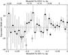 |
Fig. 8 Best-fit equivalent width (EW) of an iron 1s–2p absorption line for the present spectrum taken with the HEG. The lower x-axis corresponds to the blueshift of an Fe xxv line, the upper x-axis to that of an Fe xxvi line. In this plot positive EW corresponds to emission, negative EW to absorption. Filled squares: present HEG data; open circles: the three components reported by Cappi et al. (2009); star: the component discussed by Ponti et al. (2009). |
7.2. Other possible ultra-fast outflow signatures
The Chandra LETGS spectrum of Mrk 509 taken in 2009 showed a few weak features in the 5–9 Å band that might be associated with highly ionised gas outflowing at about −14 500 km s-1 (Ebrero et al. 2011). The strongest features would be the 1s–2p transitions of Mg xii, Si xiv and S xv. While such a component is only significant at the 90% confidence level, its outflow velocity coincides with the velocity of one of the highly ionised outflowing components seen in the iron line as reported by Ponti et al. (2009). This provides sufficient motivation to inspect our HETGS spectrum carefully.
Best-fit column densities in 1020 m-2 for highly ionised ions at −14 500 km s-1.
We have added, similar to Ebrero et al. (2011), a slab component to our best-fit model of the HETGS spectrum, with velocity dispersion frozen to 100 km s-1 and outflow velocity to −14 500 km s-1. The slab model accounts for the transmission of a layer of material composed of ions with adjustable ionic column densities. The best-fit column densities are reported in Table 5. We find no evidence of such a component. Our upper limits are more than an order of magnitude lower than those reported by Ebrero et al. (2011). For proto-solar abundances, they correspond to an equivalent hydrogen column density of < 3 × 1024 m-2 at a typical ionisation parameter of log ξ = 3.
8. Discussion
8.1. Wavelength scale
In Kaastra et al. (2011a) we paid a lot of attention to obtaining the proper wavelength scale for the RGS spectra, because of small systematic uncertainties of the order of 7 mÅ. In the present work we have found that the velocities based on the RGS spectra reported by Detmers et al. (2011) need to be increased by +55 ± 21 km s-1 to bring them into agreement with the HETGS scale. The absolute wavelength accuracy of the MEG grating as reported in the Chandra observatory guide is 11 mÅ, corresponding to about 150 km s-1 for the oxygen lines. However, the relative uncertainty is only 2 mÅ or 30 km s-1 within and between observations. We think the latter may better represent the uncertainty for our observations. The correction of +55 km s-1 corresponds to +3.7 mÅ at a typical wavelength of 20 Å; adjusting the RGS wavelength scale indicators in Table 11 of Kaastra et al. (2011a) with this number brings them all in good agreement, where we need to assume that most hot gas in our Galaxy in the direction towards Mrk 509 is at low velocity (cf. Pinto et al. 2012). The only exception is the 1s–2p line of O i from our Galaxy, that is off by about 10 mÅ. Perhaps this line suffers from more blending by weak lines from the outflow of Mrk 509 than we have accounted for.
8.2. Gas outflowing at –700 km s-1 or higher
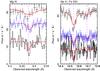 |
Fig. 9 Observed spectra near the strongest Mg xi (left panel) and Ne x (12.54 Å) and Fe xxi (12.69 Å) transitions (right panel). Spectra from top to bottom: RGS, MEG and HEG. For clarity of display we have omitted error bars on the HEG spectra; all spectra have an arbitrary offset in the y-direction, and for better visibility of the weak lines the RGS spectra have in addition been multiplied by a factor of 5 in both panels. The model spectra (thick solid histograms) represent the best-fit HETGS spectrum; for the RGS this model has been simply folded through the RGS data. |
One of the motivations for our present observation was to confirm the presence of the tentative velocity component at −715 ± 109 km s-1 in the RGS spectrum (Detmers et al. 2011). That component was visible in the strongest transitions of Mg xi, Fe xx and Fe xxi. The HETGS line profiles of Mg xi, Mg xii and other highly ionised ions do not show such a component (Fig. 1), and this is confirmed by our spectral fits that tend to give only upper limits for column densities at such velocities.
Is the high-velocity component found by Detmers et al. (2011) real? To address this question, we show the RGS and HETGS spectra near the strongest transitions from Mg xi and Fe xxi (Fig. 9). Compared to the best-fit HETGS model, the RGS spectrum shows two data bins, each about 1σ below the model, at the blue side from the centre of the line. In a fit to RGS data alone, these tend to make the outflow velocity higher indeed, but the excess is not very significant compared to the HETGS model. For Fe xxi a roughly similar situation occurs, and combining this weak blue excess absorption for both lines creates the −715 km s-1 component. Our work shows that such a component is not present in the 2012 HETGS spectrum, but of course we cannot exclude that such a somewhat weaker, but transient component was present in the 2009 RGS data.
Another indicator for possible high-velocity gas is the O viii 1s–2p line profile in the MEG spectrum, that appears to indicate a blue tail extending out to about −600 km s-1 or perhaps even beyond −1000 km s-1. Again, a global spectral fit does not confirm this, although the detailed line profile (Fig. 3) does not exclude the presence of a small amount of O viii ions around −600 km s-1.
8.3. Covering factor of the outflow
In Sect. 4 we have investigated the line profiles of the O viii Lyman series. According to the modelling of Detmers et al. (2011), this ion is produced for about 75% in the ionisation components C, and 16% and 8% in the ionisation components D and E, respectively.
We first consider the outflow components around −240 (C2 and D2) and −405 km s-1 (E2). Our analysis shows that, on average, there is some evidence that the covering factor is less than unity. At ν< −100 km s-1, the average covering factor is 0.81 ± 0.08. We note that also the UV C iv and N v lines in the same velocity range show some evidence of covering factors less than unity (Kriss et al. 2011; Arav et al. 2012), but the detailed covering factor profile is hard to determine for O viii.
A lower than unity covering factor might be caused by either a patchy outflow, or by contributions to the continuum emission outside the region covered by the outflow. We first consider this second possibility. Because components C and D of the outflow have distances of > 70 pc and 5−33 pc, respectively (Kaastra et al. 2012), and the inclination angle is likely to be in the range of 20−40 degrees, the extent of the outflow perpendicular to the line of sight will be of the order of 2−40 pc or more. Thus, if the outflow covers the continuum source only partially, there should be a significant (of the order of 10%) continuum X-ray flux contribution at distances of the order of 2−40 pc from the nucleus. The torus region would be a likely candidate, but in order to get a strong reflected X-ray flux from this region one would need a high ionisation parameter in addition to a sizeable sustained solid angle with respect to the nucleus. For such a high ionisation parameter significant atomic edges should be present in the reflected spectrum, and these cannot be relativistically blurred at such large distances from the nucleus. Our RGS spectrum also shows no evidence of strong edges.
Thus, a somewhat patchy outflow may be a better explanation for the slightly reduced covering factor, but we must stress here that the significance of fc< 1 in this velocity range is ~ 2.4σ, so there is a small probability that the covering factor is 1 and that the column density is on the lower side in order to make the O viii line core not completely black.
We next consider the velocity range between −100 and +200 km s-1, around the low velocity components. Here the average covering factor for O viii is 0.90 ± 0.08, hence it is hard to draw firm conclusions. At even higher redshifts, for velocities > 200 km s-1 the covering factor appears to be significantly smaller, about 0.3. However, in the UV lines there is no evidence of gas at these velocities, and most of the low covering factor is caused by the single bin at + 600 km s-1. At these velocities there is some weak blending with Fe xii transitions; this ion peaks at about the same ionisation parameter as O viii and according to the model of Detmers et al. (2011) it can contribute a few percent to the transmission of the O viii 1s–3p line around 16.03 Å rest frame energy.
8.4. Variability
Our analysis in Sect. 5 shows that, within the statistical uncertainties, there have been no changes in the derived column densities of most regular outflow components. The only exception appear to be components C2 and D2, both at −240 km s-1 and with log ξ at 2.07 and 2.66, respectively. Component D2 is the only X-ray component that showed significant long-term variability (Kaastra et al. 2012), and at a distance between 5–33 pc it is also the component nearest to the central black hole. In the three years between 2009 and 2012 it may well be that fresh material has entered the outflow in this component, if it is near its lower limit distance of 15 light years (5 pc). For component C2 such an explanation is unlikely, given its distance of > 70 pc. We note that components C2 and D2 are close to unstable branches of the cooling curve (Detmers et al. 2011); thus, depending on the luminosity history, gas may have moved from one ionisation parameter to another. We note that the loss of column density for component C2 is about the gain in column density for component D2. Lacking more regular monitoring of Mrk 509, however, we cannot test such a scenario.
8.5. Abundances
Our best-fit abundances do not differ much from those reported by Steenbrugge et al. (2011) based on the RGS data. We refer to that paper for a full discussion on the abundances. In general, inclusion of the HETGS data improves the accuracy, in particular for Ne, Mg, Si and Fe. The Mg and S abundances are somewhat closer to the proto-solar values by including the HETGS data.
8.6. Fe-K emission line
The spectrum clearly shows a narrow emission line component. Its flux is consistent with the values found by Yaqoob & Padmanabhan (2004) and Ponti et al. (2013), and its steadiness in flux over the years points to an origin far away from the nucleus.
The narrow iron line at 6.4 keV appears to have an extended red wing extending down to about 6.25 keV (Fig. 6). This looks quite similar to a Compton shoulder, and for that reason we have attempted a fit with a flat profile (Sect. 6). This gives a remarkable good fit to the observed profile, but the shoulder has about two times more photons than the narrow line. All models calculated by Matt (2002) for Compton shoulders have a shoulder to line ratio f less than 0.4 for transmission models and f< 0.2 for reflection models. We can clearly exclude a transmission model here, because that would give significant low-energy absorption that is not observed. Hence, there is a mismatch of a factor of 10 in the observed value for f compared to the models. This is even stronger if we consider that the equivalent width of the narrow emission line is small (16 eV), and for such a small value the models of Matt (2002) even produce a lower value f< 0.10. Despite the good fit, it thus appears hard to explain the red wing with a Compton shoulder, and we therefore have to seek another explanation for this red wing.
The full width of the red wing is about 7000 km s-1. This is smaller, but of a similar order to the line width detected by Ponti et al. (2013). If we would assume that this emission stems from an X-ray broad line region, and that there should be a similar blue wing, then the absence of such a blue wing in the observed spectrum might be explained by absorption. Partial absorption of the blue wing due to an outflow is also seen in the Lyα line of hydrogen, for example Kriss et al. (2011). However that absorption extends only up to −500 km s-1 in the UV spectrum. Here we would need absorption at several thousands of km s-1. To absorb the blue wing, we would need ionisation stages containing Fe xviii or higher, having 1s–2p transitions above 6.4 keV. However, application of our xabs models shows that this is impossible: we would also get significant 1s–3p transitions at higher energies, and the required column densities, of the order of 1028 m-2 for hydrogen, are inconsistent with the column densities that we derived from our fits to the low-energy part of the spectrum. We conclude that if the red wing of the narrow Fe-K emission line has an origin in an X-ray broad line region, then the line must be asymmetric with significantly more flux in the red wing.
Another possibility is that the red wing is not a separate entity but part of a broader structure, for instance a weak relativistic emission line. Indeed, we get an excellent fit to the spectrum using the sum of the narrow component with a relativistically broadened iron line. Such a line could stem from reflection by relatively cool material. The line is weak, however, and therefore poorly constrained, and the interpretation of the best-fit parameters must be done with care. The inclination angle seems to be small, perhaps about 20 degrees, which is consistent with a type 1 viewing direction, and with the fact that, for instance, from the optical imaging of the O iii lines (Phillips et al. 1983) it appears as if we are looking fully through the ionisation cone.
This relativistic line could be part of a more general reflection component. Our best-fit reflection fraction R of 0.64 ± 0.11 then suggests that the covering of this reflector is less than 2π sr.
From their analysis of the XMM-Newton pn data, Ponti et al. (2013) also concluded that the spectrum allows for a weak relativistic emission line. However, in their case the relativistic line originates from Fe xxv or Fe xxvi while we need colder iron. In the case of Ponti et al. (2013) the data could be modelled alternatively with ionised Fe xxv and Fe xxvi emission lines. Our data are consistent with such a model.
8.7. Ultra-fast outflows
The HETGS spectrum shows no clear evidence of ultra-fast outflows in the form of highly blueshifted absorption lines of Fe xxv and Fe xxvi. In Sect. 7.1 we showed that the presence of such lines is not statistically significant at the expected blueshifts for an ultra-fast outflow. However, given the statistical uncertainties we also cannot rule out such lines at the strength of about 20 eV equivalent width as reported by Cappi et al. (2009). For this equivalent width, we derive a hydrogen column density of 1.2 × 1026 and 3.1 × 1026 m-2 for Fe xxv and Fe xxvi, respectively. These values are two orders of magnitude higher than those measured for the ionisation components A to E, which are of the order of a few times 1024 m-2 (see Table 2). We can see in Fig. 4 that the measured hydrogen column density of the absorbers in general increases with the ionisation parameter, a behaviour often seen in other AGN (Behar 2009). However, for values of log ξ of 3.7 and 4.1 (for which the concentration of Fe xxv and Fe xxvi peak, respectively) one would expect columns of the order of ~1025 m-2, much smaller than found for the ultra-fast outflows. This supports the idea that the ultra-fast outflows, if present, may originate in a different environment than the warm absorbers, possibly in winds launched close to the accretion disc.
Similarly, troughs of Mg xii, Si xiv and S xv outflowing at ~0.05c were marginally detected in the LETGS spectrum in the 5–9 Å range (Ebrero et al. 2011). This velocity was remarkably similar to that of the variable Fe absorption lines reported by Ponti et al. (2009), suggesting that both absorbers might belong to the same ionised wind. While the lack of a significant detection could be attributed to the low sensitivity of LETGS at those wavelengths, one would expect to detect them significantly in the HETGS if they are actually present. However, we did not find evidence of any of these absorption features in our spectrum, obtaining tighter upper limits on their column densities than those of Ebrero et al. (2011). These ions are typically produced in a gas with ionisation parameter log ξ ~ 3, very close to that of component E2. The expected hydrogen column density is also similar to that measured for component E2, which is significantly detected in our spectrum. Therefore, if such an ionised wind was present in this observation it would have been detected.
In summary, we do not find significant evidence of an ultra-fast outflow in this Chandra HETGS observation of Mrk 509, in spite of previous detections by Cappi et al. (2009) and Ponti et al. (2009). This result is in line with the observation of no signatures of such outflows in the combined 600 ks XMM-Newton pn spectrum, with the exception of a marginal detection of two absorption features at 9 keV and 10.2 keV (Ponti et al. 2013) during observation 4 which could be attributed to Fe xxvi outflowing at ~ −0.3c. However, the lack of detection of such outflows during this campaign may not rule out their existence. Ultra-fast outflows are thought to originate very close to the accretion disc, at distances typically of hundreds of Schwarzschild radii (Tombesi et al. 2012). Time variability is therefore an important structural feature of these winds that may cause them to change face dramatically at timescales of hours and days, thus preventing them from being detected in all observations. More sensitive observations (e.g. ASTRO-H) are needed to get a more conclusive view on ultra-fast outflows.
9. Conclusions
In this paper we report a Chandra HETGS observation of Mrk 509 taken in September 2012. The analysis of the HETGS spectrum confirms the structure of the warm absorber measured with XMM-Newton RGS in 2009 by Detmers et al. (2011), who found 5 distinct ionisation components in two kinematic regimes.
We find no evidence of an outflow component at −715 km s-1 as reported by Detmers et al. (2011) for the RGS spectrum. Most likely a few statistical outliers at the blue wing of the Mg xi and Fe xxi lines caused the apparent blueshift in the RGS spectrum, although we cannot exclude that is was a transient feature.
We find no significant variability in the physical properties of the absorbers between the 2009 and 2012 observations, except for the components C2 and D2 at −240 km s-1, where the column density of the lower ionisation component C2 decreased in favour of the higher ionisation component D2.
The analysis of the line profiles of the O viii Ly-series shows evidence that the covering factor is less than unity. We obtain an average covering factor of 0.81 ± 0.08 for outflow velocities faster than −100 km s-1, similar to the values found in the UV for C iv and N v lines. This can be interpreted as a patchy wind that leaks part of the underlying continuum, although the significance of fc< 1 is just above the 2σ level.
We also modelled the Fe-K emission. The parameters of the narrow component are consistent with those determined by Ponti et al. (2013), and its steadiness in flux between 2009 and 2012 points out to an origin distant from the central engine. We see a strong red wing at the low energy side of the narrow line. It is too strong for a Compton shoulder, and it is unlikely to be a symmetric broad line that is completely absorbed on the blue side. Rather, it points towards an intrinsically asymmetric broadened line, for instance a weak relativistic line.
Our HETGS spectrum shows no evidence of ultra-fast outflows in the Fe-K region nor in the 3 keV region. The lack of detection of these features, previously reported in other Mrk 509 observations (Dadina et al. 2005; Cappi et al. 2009; Ponti et al. 2009), might be due to intrinsic time variability, as they are formed very close to the accretion disc.
See tgcat.mit.edu.
Acknowledgments
This work is based on observations obtained with XMM-Newton, an ESA science mission with instruments and contributions directly funded by ESA Member States and the USA (NASA). It is also based on observations with INTEGRAL, an ESA project with instrument and science data centre funded by ESA member states (especially the PI countries: Denmark, France, Germany, Italy, Switzerland, Spain), Czech Republic, and Poland and with the participation of Russia and the USA. This work made use of data supplied by the UK Swift Science Data Centre at the University if Leicester. SRON is supported financially by NWO, the Netherlands Organization for Scientific Research. J.S. Kaastra thanks the PI of Swift, Neil Gehrels, for approving the TOO observations. M. Mehdipour acknowledges the support of Studentship Enhancemement Program (STEP) awarded by the UK Science & Technology Facilities Council (STFC). N. Arav and G. Kriss gratefully acknowledge support from NASA/XMM-Newton Guest Investigator grant NNX09AR01G. Support for HST Program numbers 12022 and 12916 was provided by NASA through grants from the Space Telescope Science Institute, which is operated by the Association of Universities for Research in Astronomy, Inc., under NASA contract NAS5-26555. E. Behar was supported by a grant from the ISF. S. Bianchi, M. Cappi, and G. Ponti acknowledge financial support from contract ASI-INAF n. I/088/06/0. P.-O. Petrucci acknowledges financial support from CNES and from the Franco-Italian PICS of the CNRS. G. Ponti acknowledges support via EU Marie Curie Intra-European Fellowships under contract no. FP7-PEOPLE-2009-IEF-331095 and FP-PEOPLE-2012-IEF-331095.
References
- Arav, N., Korista, K. T., & de Kool, M. 2002, ApJ, 566, 699 [NASA ADS] [CrossRef] [Google Scholar]
- Arav, N., Edmonds, D., Borguet, B., et al. 2012, A&A, 544, A33 [NASA ADS] [CrossRef] [EDP Sciences] [Google Scholar]
- Behar, E. 2009, ApJ, 703, 1346 [NASA ADS] [CrossRef] [Google Scholar]
- Cappi, M., Tombesi, F., Bianchi, S., et al. 2009, A&A, 504, 401 [NASA ADS] [CrossRef] [EDP Sciences] [Google Scholar]
- Chartas, G., Brandt, W. N., Gallagher, S. C., & Garmire, G. P. 2002, ApJ, 579, 169 [NASA ADS] [CrossRef] [Google Scholar]
- Chartas, G., Brandt, W. N., & Gallagher, S. C. 2003, ApJ, 595, 85 [NASA ADS] [CrossRef] [Google Scholar]
- Crenshaw, D. M., Kraemer, S. B., Boggess, A., et al. 1999, ApJ, 516, 750 [NASA ADS] [CrossRef] [Google Scholar]
- Crenshaw, D. M., Kraemer, S. B., & George, I. M. 2003, ARA&A, 41, 117 [NASA ADS] [CrossRef] [Google Scholar]
- Dadina, M., Cappi, M., Malaguti, G., Ponti, G., & de Rosa, A. 2005, A&A, 442, 461 [NASA ADS] [CrossRef] [EDP Sciences] [Google Scholar]
- Detmers, R. G., Kaastra, J. S., Steenbrugge, K. C., et al. 2011, A&A, 534, A38 (Paper III) [NASA ADS] [CrossRef] [EDP Sciences] [Google Scholar]
- Ebrero, J., Kriss, G. A., Kaastra, J. S., et al. 2011, A&A, 534, A40 (Paper V) [NASA ADS] [CrossRef] [EDP Sciences] [Google Scholar]
- Elvis, M. 2000, ApJ, 545, 63 [NASA ADS] [CrossRef] [Google Scholar]
- Kaastra, J. S., Mewe, R., & Nieuwenhuijzen, H. 1996, in UV and X-ray Spectroscopy of Astrophysical and Laboratory Plasmas, eds. K. Yamashita, & T. Watanabe, 411 [Google Scholar]
- Kaastra, J. S., Mewe, R., Liedahl, D. A., Komossa, S., & Brinkman, A. C. 2000, A&A, 354, L83 [NASA ADS] [Google Scholar]
- Kaastra, J. S., de Vries, C. P., Steenbrugge, K. C., et al. 2011a, A&A, 534, A37 (Paper II) [NASA ADS] [CrossRef] [EDP Sciences] [Google Scholar]
- Kaastra, J. S., Petrucci, P.-O., Cappi, M., et al. 2011b, A&A, 534, A36 (Paper I) [NASA ADS] [CrossRef] [EDP Sciences] [Google Scholar]
- Kaastra, J. S., Detmers, R. G., Mehdipour, M., et al. 2012, A&A, 539, A117 (Paper VIII) [NASA ADS] [CrossRef] [EDP Sciences] [Google Scholar]
- Kazanas, D., Fukumura, K., Behar, E., Contopoulos, I., & Shrader, C. 2012, Astron. Rev., 7, 92 [Google Scholar]
- Kriss, G. A., Arav, N., Kaastra, J. S., et al. 2011, A&A, 534, A41 (Paper VI) [NASA ADS] [CrossRef] [EDP Sciences] [Google Scholar]
- Krolik, J. H., & Kriss, G. A. 2001, ApJ, 561, 684 [NASA ADS] [CrossRef] [Google Scholar]
- Lodders, K., & Palme, H. 2009, Meteoritics and Planetary Science Supplement, 72, 5154 [Google Scholar]
- Magdziarz, P., & Zdziarski, A. A. 1995, MNRAS, 273, 837 [NASA ADS] [CrossRef] [Google Scholar]
- Matt, G. 2002, MNRAS, 337, 147 [NASA ADS] [CrossRef] [Google Scholar]
- Phillips, M. M., Baldwin, J. A., Atwood, B., & Carswell, R. F. 1983, ApJ, 274, 558 [Google Scholar]
- Pinto, C., Kriss, G. A., Kaastra, J. S., et al. 2012, A&A, 541, A147 (Paper IX) [NASA ADS] [CrossRef] [EDP Sciences] [Google Scholar]
- Ponti, G., Cappi, M., Vignali, C., et al. 2009, MNRAS, 394, 1487 [NASA ADS] [CrossRef] [Google Scholar]
- Ponti, G., Cappi, M., Costantini, E., et al. 2013, A&A, 549, A72 (Paper XI) [NASA ADS] [CrossRef] [EDP Sciences] [Google Scholar]
- Steenbrugge, K. C., Kaastra, J. S., Detmers, R. G., et al. 2011, A&A, 534, A42 (Paper VII) [NASA ADS] [CrossRef] [EDP Sciences] [Google Scholar]
- Tombesi, F., Cappi, M., Reeves, J. N., et al. 2010, A&A, 521, A57 [NASA ADS] [CrossRef] [EDP Sciences] [Google Scholar]
- Tombesi, F., Cappi, M., Reeves, J. N., & Braito, V. 2012, MNRAS, 422, L1 [NASA ADS] [CrossRef] [Google Scholar]
- Tombesi, F., Cappi, M., Reeves, J. N., et al. 2013, MNRAS, 430, 1102 [Google Scholar]
- Yaqoob, T., & Padmanabhan, U. 2004, ApJ, 604, 63 [NASA ADS] [CrossRef] [Google Scholar]
- Zycki, P. T., & Czerny, B. 1994, MNRAS, 266, 653 [NASA ADS] [CrossRef] [Google Scholar]
- Zycki, P. T., Done, C., & Smith, D. A. 1999, MNRAS, 305, 231 [NASA ADS] [CrossRef] [Google Scholar]
All Tables
Best-fit abundances in the outflow of Mrk 509 relative to oxygen and in proto-solar units.
All Figures
|
Fig. 1 Normalised line profiles for Si and Mg lines. Line identifications and gratings are indicated in the panels. The dotted lines correspond to the expected line profile for an infinitely narrow absorption line at outflow velocity 0 convolved with the instrumental line-spread function and with a depth corresponding to the depth of the observed spectral line. They serve to show the typical instrumental broadening. |
| In the text | |
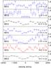 |
Fig. 2 As Fig. 1, but for Ne and O lines. |
| In the text | |
|
Fig. 3 Velocity-dependent total O viii column density N and covering factor fc (lower panels) deduced from fits (upper two panels) to the O viii Lyα and Lyβ lines. |
| In the text | |
|
Fig. 4 Best-fit column densities for a model with 28 absorption components applied to the joint RGS and HETGS spectra. Crosses with labels indicate the positions of the components found in the analysis of the RGS spectrum by Detmers et al. (2011). |
| In the text | |
|
Fig. 5 HEG spectrum near the Fe-K emission line. Shown are the residuals relative to a power-law continuum. The rest frame energies of some important transitions are indicated by dotted lines (the Fe xxv Lyα line consist of two components, and the Fe xxv triplet consists of four components, from left to right the forbidden line, the intercombination lines and the resonance line). |
| In the text | |
|
Fig. 6 HEG spectrum in 2012 near the Fe-K emission line (data points with error bars). The model (solid line) consists of a power-law, narrow emission line and two flat plateaus. |
| In the text | |
|
Fig. 7 HEG spectrum near the Fe-K emission line (data points with error bars) fitted to a model with a narrow emission line and a relativistically blurred cold reflection component. The lines are from bottom to top: contribution from the narrow emission line (solid), reflection component (dot-dashed), powerlaw component (dashed), sum of power law and reflection (dotted) and total model (solid histogram). |
| In the text | |
|
Fig. 8 Best-fit equivalent width (EW) of an iron 1s–2p absorption line for the present spectrum taken with the HEG. The lower x-axis corresponds to the blueshift of an Fe xxv line, the upper x-axis to that of an Fe xxvi line. In this plot positive EW corresponds to emission, negative EW to absorption. Filled squares: present HEG data; open circles: the three components reported by Cappi et al. (2009); star: the component discussed by Ponti et al. (2009). |
| In the text | |
|
Fig. 9 Observed spectra near the strongest Mg xi (left panel) and Ne x (12.54 Å) and Fe xxi (12.69 Å) transitions (right panel). Spectra from top to bottom: RGS, MEG and HEG. For clarity of display we have omitted error bars on the HEG spectra; all spectra have an arbitrary offset in the y-direction, and for better visibility of the weak lines the RGS spectra have in addition been multiplied by a factor of 5 in both panels. The model spectra (thick solid histograms) represent the best-fit HETGS spectrum; for the RGS this model has been simply folded through the RGS data. |
| In the text | |
Current usage metrics show cumulative count of Article Views (full-text article views including HTML views, PDF and ePub downloads, according to the available data) and Abstracts Views on Vision4Press platform.
Data correspond to usage on the plateform after 2015. The current usage metrics is available 48-96 hours after online publication and is updated daily on week days.
Initial download of the metrics may take a while.