| Issue |
A&A
Volume 570, October 2014
|
|
|---|---|---|
| Article Number | A104 | |
| Number of page(s) | 13 | |
| Section | Stellar atmospheres | |
| DOI | https://doi.org/10.1051/0004-6361/201423772 | |
| Published online | 30 October 2014 | |
Improving the surface brightness-color relation for early-type stars using optical interferometry⋆,⋆⋆
1
Laboratoire Lagrange, UMR 7293, UNS/CNRS/OCA, 06300
Nice, France
e-mail: This email address is being protected from spambots. You need JavaScript enabled to view it.
2
Laboratoire Dynamique Moléculaire et Matériaux Photoniques,
UR11ES03, Université de Tunis/ESSTT,
Tunisie
3
Departamento de Astronomía, Universidad de Concepción, Casilla
160-C, Concepción, Paraguay
4
Warsaw University Observatory, AL. Ujazdowskie 4, 00-478
Warsaw,
Poland
5
Univ. Grenoble Alpes, IPAG, 38000
Grenoble,
France
6
CNRS, IPAG, 38000
Grenoble,
France
7
Université Lyon 1, Observatoire de Lyon,
9 avenue Charles André,
69230
Saint Genis Laval,
France
8
CNRS/UMR 5574, Centre de Recherche Astroph. de Lyon, École Normale
Supérieure, 69007
Lyon,
France
9
Georgia State University, PO Box 3969, Atlanta
GA
30302-3969,
USA
10
CHARA Array, Mount Wilson Observatory,
91023
Mount Wilson
CA,
USA
Received: 7 March 2014
Accepted: 2 September 2014
Abstract
Context. The method of distance determination of eclipsing binaries consists in combining the radii of both components determined from spectro-photometric observations with their respective angular diameters derived from the surface brightness-color relation (SBC). However, the largest limitation of the method comes from the uncertainty on the SBC relation: about 2% for late-type stars (or 0.04 magnitude) and more than 10% for early-type stars (or 0.2 mag).
Aims. The aim of this work is to improve the SBC relation for early-type stars in the −1 ≤ V − K ≤ 0 color domain, using optical interferometry.
Methods. Observations of eight B- and A-type stars were secured with the VEGA/CHARA instrument in the visible. The derived uniform disk angular diameters were converted into limb darkened angular diameters and included in a larger sample of 24 stars, already observed by interferometry, in order to derive a revised empirical relation for O, B, A spectral type stars with a V − K color index ranging from −1 to 0. We also took the opportunity to check the consistency of the SBC relation up to V − K ≃ 4 using 100 additional measurements.
Results. We determined the uniform disk angular diameter for the eight following stars: γ Ori, ζ Per, 8 Cyg, ι Her, λ Aql, ζ Peg, γ Lyr, and δ Cyg with V − K color ranging from −0.70 to 0.02 and typical precision of about 1.5%. Using our total sample of 132 stars with V − K colors index ranging from about − 1 to 4, we provide a revised SBC relation. For late-type stars (0 ≤ V − K ≤ 4), the results are consistent with previous studies. For early-type stars (− 1 ≤ V − K ≤ 0), our new VEGA/CHARA measurements combined with a careful selection of the stars (rejecting stars with environment or stars with a strong variability), allows us to reach an unprecedented precision of about 0.16 magnitude or ≃7% in terms of angular diameter.
Conclusions. We derive for the first time a SBC relation for stars between O9 and A3, which provides a new and reliable tool for the distance scale calibration.
Key words: stars: early-type / techniques: interferometric / stars: distances / binaries: eclipsing / methods: observational / stars: atmospheres
Partly based on VEGA/CHARA observations.
Appendix A is available in electronic form at http://www.aanda.org
© ESO, 2014
1. Introduction
The distance measurements to extragalactic targets in the last century revolutionized our understanding of the distance scale of the universe. The distance to the Large Magellanic Cloud is a critical rung on the cosmic distance ladder, and numerous independent methods involving, for instance, RR Lyrae stars (Feast 1997; Szewczyk et al. 2008; Pietrzyński et al. 2008), Cepheids (Bohm-Vitense 1985; Evans 1991, 1992; Freedman & Madore 1996; Freedman et al. 2008), or red clump stars (Udalski et al. 1998b,a; Pietrzyński & Gieren 2002; Laney et al. 2012) have been used to derive its distance.
The main goal of the long term program called the Araucaria project is to significantly improve the calibration of the cosmic distance scale based on observations of several distance indicators in nearby galaxies (Gieren et al. 2005). Eclipsing binary systems are particularly important to provide the zero point of the extragalactic distances and study in detail populational dependence on other distance indicators like RR Lyrae stars, Cepheids, red clump stars, etc. Thirteen long period systems composed of late-type giants were analyzed in the Magellanic Clouds so far: eight in the Large Magellanic Cloud (Pietrzyński et al. 2009, 2013), and five in the Small Magellanic Cloud (Graczyk et al. 2012, 2014). For such systems, the linear dimension of both components can be measured with a precision up to of 1% from the analysis of high-quality spectroscopic and photometric data (e.g., Torres et al. 2010). The distance to an eclipsing binary follows from the dimensions determined in this way, plus the angular diameters derived from the absolute surface brightness, which is very well calibrated for late-type stars (Di Benedetto 2005). This conceptually very simple technique very weakly depends on reddening and metallicity, and provides the most accurate tool for measuring distances to nearby galaxies (Pietrzyński et al. 2013; Graczyk et al. 2014).
However the heart of this method, the surface brightness-color (SBC) relation, is very well calibrated only for late-type stars which significantly limits its usage. The late-type systems composed of main-sequence stars are usually faint, while those composed of giants have very long periods (several hundred days) that makes them very difficult to find. As a result, only about 45 late-type systems, well suited to precise distance determination have been discovered so far in the Magellanic Clouds by the Optical Gravitational Microlensing Experiment (OGLE; Pawlak et al. 2013; Graczyk et al. 2011). On the other hand, many more relatively bright systems are known in nearby galaxies (Massey et al. 2013; Graczyk et al. 2011; Wyrzykowski et al. 2003, 2004; Bonanos et al. 2006; Macri et al. 2001; Mochejska et al. 2001; Vilardell et al. 2006; Pawlak et al. 2013). Therefore, in order to derive the distance to nearby galaxies and to study the geometry of the Magellanic Clouds, it is imperative to calibrate SBC relation for early-type stars.
The purpose of this paper is to improve the SBC relation for early-type stars by using the resolving power of the Visible spEctroGraph and polArimeter (VEGA) beam combiner (Mourard et al. 2009) operating at the focus of the Center for High Angular Resolution Astronomy (CHARA) Array (ten Brummelaar et al. 2005) located at Mount Wilson Observatory (California, USA). The CHARA array consists of six telescopes of 1 m in diameter, configured in a Y shape, which offers 15 different baselines from 34 m to 331 m. These baselines can achieve a spatial resolution up to 0.3 mas in the visible which is necessary in order to resolve early-type stars. Early-type stars are very small in terms of angular diameter and can be affected by several physical phenomena, like fast rotation, winds, and environment, which can potentially bias the interferometric measurements.
Physical parameters of the stars in our sample.
This paper is structured as follows. Section 2 is devoted to a description of the stars in our sample. In Sect. 3, we present the data reduction process and the method used to derive the angular diameters. Section 4 is dedicated to the calibration of the SBC relation, and we discuss our results in Sect. 5. We draw conclusions in Sect. 6.
2. VEGA/CHARA observations of eight early-type stars
We carefully selected eight early-type stars with a (V − K) color index ranging from −0.70 to 0.02. They are north hemisphere main-sequence subgiant and giant stars (δ> 4°) with spectral types ranging from B1 to A1. They are much brighter (with a visual magnitude mV ranging from 1.6 to 4.7) than the limiting magnitude of VEGA (about mV = 7 in medium spectral resolution). They are also bright in the K band (with a mK magnitude lower than 5.1) which makes it possible to track the fringes simultaneously with the infrared CLIMB combiner (Sturmann et al. 2010). All the apparent magnitudes in V and K bands that we have collected from the literature are in the Johnson system (Johnson et al. 1966; see also Mermilliod et al. 1997). The accuracy of their parallaxes π spans from 1.5% to 15%. The color excess E(V − K), the visual absorption AV, the effective temperature Teff, the mass M, the radius R, the luminosity L, the surface gravity log g, and the metallicity index [ Fe/H ] are listed in Table 1. We emphasize that for our purpose (limb-darkening estimates; see end of Sect. 3.1), we do not need very precise estimates of the fundamental parameters of the stars in our sample, which explains why we do not provide any uncertainty on these parameters in the second part of Table 1.
Among the eight early-type stars in our sample, there are six low rotators (λ Aql, γ Ori, γ Lyr, ι Her, 8 Cyg, and ζ Per) and two fast rotating stars (δ Cyg and ζ Peg). In the following, we define fast rotators as stars with vrotsini> 75 km s-1. A theoretical study which aims at quantifying the impact of fast rotation on the SBC relation for early-type stars is currently in progress and will be published in a forthcoming paper.
We observed our sample stars from July 23, 2011, to August 29, 2013, using different suitable triplets available on the CHARA array. A summary of the observations is given in Table 2.
3. The limb-darkened angular diameters
In this section, we describe how we derive the limb-darkened angular diameter for all the stars in our sample.
3.1. Data reduction and methodology
The first step is to calibrate the visibility measurements of our targets using
observations of reference stars. These calibrators (Table 3) were selected using the SearchCal1
software developed by the Jean-Marie Mariotti Center (JMMC; Bonneau et al. 2006). The way this calibration is done is shown in Fig. 1 in the case of γ Lyr (data obtained on
June 21, 2012, with the E1E2W2 three-telescope configuration). We used the standard
sequence C6-S-C6 in which S is the target and C6 is the reference star. The light blue
dots are the raw visibilities obtained on the science star for the three corresponding
baselines: E2E1 (upper panel), E2W2 (middle panel), and E1W2 (bottom panel). Our VEGA
measurements are typically divided into 30 blocks of observations, and each block contains
1000 images with an exposure time of 15 millisec. For each block, the raw squared
visibility is calculated using the auto-correlation mode (Mourard et al. 2009, 2011). The red dots
in the figure represent the transfer function obtained by comparing the expected
visibility of the reference star to the one that has been measured. This transfer function
is then used to calibrate the visibilities obtained on the science target (blue dots). A
cross-check of the quality of the transfer function is usually done for several bandwidths
and over the whole night. Under good seeing conditions, the transfer function of
VEGA/CHARA is generally stable at the level of 2% for more than one hour. The squared
calibrated visibilities  obtained from our VEGA observations are
listed in Tables A.1. The systematic uncertainties
that stem from the uncertainty on the reference stars are negligible compared to the
statistical uncertainties, and are neglected in the rest of this study.
obtained from our VEGA observations are
listed in Tables A.1. The systematic uncertainties
that stem from the uncertainty on the reference stars are negligible compared to the
statistical uncertainties, and are neglected in the rest of this study.
Summary of the observing log.
Reference stars and their parameters, including the spectral type, the visual magnitude (mV), and the predicted uniform disk angular diameter (in mas) derived from the JMMC SearchCal software (Bonneau et al. 2006).
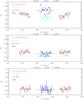 |
Fig. 1 Time sequences of raw visibilities of the science observations (light blue dots), calibrated (blue dots) using the transfer function (red dots). |
The calibrated visibility curves obtained for each star in our sample (Fig. 2) are then used to constrain a model of uniform disk,
that contains only one parameter, the so-called uniform disk angular diameter
(θUD). This is performed using the
LITpro2 software developed by the JMMC (Tallon-Bosc et al. 2008). The following formula of
Hanbury Brown et al. (1974b) provides an
analytical way to convert the equivalent uniform disk angular diameter θUD into the
limb-darkened disk θLD:![Mathematical equation: \begin{equation} \theta_{\mathrm{LD}}(\lambda)=\theta_{\mathrm{UD}}(\lambda)\left[ \frac{(1-\frac{U_{\lambda}}{3})}{(1-\frac{7U_{\lambda}}{15})} \right] ^{\frac{1}{2}}\cdot \end{equation}](/articles/aa/full_html/2014/10/aa23772-14/aa23772-14-eq143.png) (1)For each star, the limb-darkening coefficient
Uλ is derived from the
numerical tables of Claret & Bloemen (2011).
These tables are based on the ATLAS (Kurucz 1970)
and PHOENIX (Hauschildt et al. 1997) atmosphere
models. The input parameters of these tables are the effective temperature
(Teff), the metallicity ([ Fe/H ]), the surface gravity
(log g),
and the micro-turbulence velocity. The steps for these quantities are 250 K, 0.5, 0.5, and
2 km s-1,
respectively. The three first parameters are given in Table 1 and were rounded, for each star, to the closest value found in the
table of Claret. The micro-turbulence velocity has almost no impact on the derived
limb-darkened diameter (fifth decimal). We took arbitrarily 8 km s-1 for stars with Teft> 15 000
K and 4 km s-1for
stars with Teft
< 15 000 K. We also consider the limb-darkening coefficient
applicable to the R band of VEGA (UR in the
following).
(1)For each star, the limb-darkening coefficient
Uλ is derived from the
numerical tables of Claret & Bloemen (2011).
These tables are based on the ATLAS (Kurucz 1970)
and PHOENIX (Hauschildt et al. 1997) atmosphere
models. The input parameters of these tables are the effective temperature
(Teff), the metallicity ([ Fe/H ]), the surface gravity
(log g),
and the micro-turbulence velocity. The steps for these quantities are 250 K, 0.5, 0.5, and
2 km s-1,
respectively. The three first parameters are given in Table 1 and were rounded, for each star, to the closest value found in the
table of Claret. The micro-turbulence velocity has almost no impact on the derived
limb-darkened diameter (fifth decimal). We took arbitrarily 8 km s-1 for stars with Teft> 15 000
K and 4 km s-1for
stars with Teft
< 15 000 K. We also consider the limb-darkening coefficient
applicable to the R band of VEGA (UR in the
following).
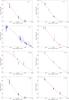 |
Fig. 2 Squared visibility versus spatial frequency for all stars in our sample with their corresponding statistical uncertainties. The red solid lines indicate the best uniform disk model obtained from the LITpro fitting software. |
Angular diameters obtained with VEGA/CHARA and the corresponding surface brightness.
3.2. Results
The uniform disk angular diameter (θUD), the limb-darkening coefficients
(UR), and the derived limb-darkened angular
diameters (θLD) are listed in Table 4 for each star in our sample. The value of
θLD ranges from 0.31 mas to 0.79 mas, with
a relative precision from 0.5% to 3.5% (average of 1.5%). The reduced
 is from 0.4 to 2.9 depending on the
dispersion of the calibrated visibilities. For γ Lyr, our result (θUD = 0.742 ±
0.010 mas) agrees at the 1σ level with the measurements from the PAVO/CHARA
instrument (θUD =
0.729 ± 0.008 mas, Maestro et al.
2013). For γ Ori, our angular diameter (θLD = 0.715 ±
0.005 mas) is consistent with the value derived from the Narrabri
Stellar Intensity Interferometer (NSII) (θLD = 0.72 ± 0.04 mas, Hanbury Brown et al. 1974a). For other stars with
angular diameters lower than 0.6 mas (ι Her, λ Aql, 8 Cyg, and ζ Per) and for the two fast
rotators (ζ
Peg and δ
Cyg) there are no interferometric observations available to our knowledge.
is from 0.4 to 2.9 depending on the
dispersion of the calibrated visibilities. For γ Lyr, our result (θUD = 0.742 ±
0.010 mas) agrees at the 1σ level with the measurements from the PAVO/CHARA
instrument (θUD =
0.729 ± 0.008 mas, Maestro et al.
2013). For γ Ori, our angular diameter (θLD = 0.715 ±
0.005 mas) is consistent with the value derived from the Narrabri
Stellar Intensity Interferometer (NSII) (θLD = 0.72 ± 0.04 mas, Hanbury Brown et al. 1974a). For other stars with
angular diameters lower than 0.6 mas (ι Her, λ Aql, 8 Cyg, and ζ Per) and for the two fast
rotators (ζ
Peg and δ
Cyg) there are no interferometric observations available to our knowledge.
For the two rotators, we derive the apparent oblateness using the approximate relation
provided by van Belle et al. (2006), their Eq. (A1)
 , where Rb,
Ra, M, and G are the major and minor
apparent radius of the star, its mass, and the gravitational constant. We find
, where Rb,
Ra, M, and G are the major and minor
apparent radius of the star, its mass, and the gravitational constant. We find
 for ζ Peg considering
 and M = 3.22
M⊙, where
and M = 3.22
M⊙, where
 is the mean radius (see Table 1), while the rotational projected velocity
vsini is set to 140
km s-1(Abt et al. 2002). For δ Cyg, we find similarly
is the mean radius (see Table 1), while the rotational projected velocity
vsini is set to 140
km s-1(Abt et al. 2002). For δ Cyg, we find similarly
 considering vsini =
140 km s-1(Slettebak et al.
1975; Gray 1980; Carpenter et al. 1984; Abt & Morrell
1995; Abt et al. 2002; van Belle 2012). Consequently, our data might be
sensitive to the expected gravity darkening intensity distribution and the flatness of the
star. However, this also depends on the baseline orientation. For both stars, the three
telescopes (Table 2) are aligned. Thus, even if our
reduced are rather low (1.7 for ζ Peg and 1.2 for
δ Cyg), we
cannot exclude a bias on our derived limb-darkened angular diameters. In order to get a
rough estimate of this bias, we only consider in first approximation the oblateness of the
star while the gravity darkening is set to be negligible. As a consequence, if the
orientation of the baseline is aligned with the polar or equatorial axis, we can estimate
a maximum systematic error of about 0.039 mas (6%) for ζ Peg, while we find 0.047 mas (7%) for δ Cyg. We translate these
uncertainties in terms of Sv magnitude in Sect.
4.
considering vsini =
140 km s-1(Slettebak et al.
1975; Gray 1980; Carpenter et al. 1984; Abt & Morrell
1995; Abt et al. 2002; van Belle 2012). Consequently, our data might be
sensitive to the expected gravity darkening intensity distribution and the flatness of the
star. However, this also depends on the baseline orientation. For both stars, the three
telescopes (Table 2) are aligned. Thus, even if our
reduced are rather low (1.7 for ζ Peg and 1.2 for
δ Cyg), we
cannot exclude a bias on our derived limb-darkened angular diameters. In order to get a
rough estimate of this bias, we only consider in first approximation the oblateness of the
star while the gravity darkening is set to be negligible. As a consequence, if the
orientation of the baseline is aligned with the polar or equatorial axis, we can estimate
a maximum systematic error of about 0.039 mas (6%) for ζ Peg, while we find 0.047 mas (7%) for δ Cyg. We translate these
uncertainties in terms of Sv magnitude in Sect.
4.
4. The calibration of the surface brightness relation
4.1. Methodology
As already mentioned in the introduction, the SBC relation is a very robust tool for the
distance scale calibration. The surface brightness SV of a star is
linked to its visual intrinsic dereddened magnitude mV0 and its
limb-darkened angular diameter θLD by the following relation:
 (2)Instead of SV, the surface
brightness parameter FV =
4.2207−0.1SV is often
adopted in the literature to determine the stellar angular diameters (Barnes & Evans 1976). In order to derive
mV0, we
first selected the apparent mV magnitudes for all
the stars in our sample (Mermilliod et al. 1997).
These magnitudes are expressed in the Johnson system (Johnson et al. 1966) and their typical uncertainty is of about 0.015 mag. In order to correct these
magnitudes from the reddening we then use the following formulae mV0 =
mV −
AV, where
AV is the extinction in
the V band.
Determining the extinction is a difficult task. We adopt the following strategy. For stars
lying closer than 75 pc we use the simple relation
(2)Instead of SV, the surface
brightness parameter FV =
4.2207−0.1SV is often
adopted in the literature to determine the stellar angular diameters (Barnes & Evans 1976). In order to derive
mV0, we
first selected the apparent mV magnitudes for all
the stars in our sample (Mermilliod et al. 1997).
These magnitudes are expressed in the Johnson system (Johnson et al. 1966) and their typical uncertainty is of about 0.015 mag. In order to correct these
magnitudes from the reddening we then use the following formulae mV0 =
mV −
AV, where
AV is the extinction in
the V band.
Determining the extinction is a difficult task. We adopt the following strategy. For stars
lying closer than 75 pc we use the simple relation  (3)where π is the parallax of the
stars [in mas]. This equation is standard in the literature (Blackwell et al. 1990; Di Benedetto
1998, 2005). The corresponding uncertainty
is set to 0.01 mag.
(3)where π is the parallax of the
stars [in mas]. This equation is standard in the literature (Blackwell et al. 1990; Di Benedetto
1998, 2005). The corresponding uncertainty
is set to 0.01 mag.
For distant stars we derive the absorption using the (B − V)
extinction (Laney & Stobie 1993):  (4)The difficulty is then to derive
E(B −
V). We have several possibilities. First, we use the
so-called Q
method, with Q =
(U − B) − 0.72(B −
V), which was originally proposed by Johnson & Morgan (1953). The value of
Q is
derived for each star using observed UBV magnitudes from (Ducati 2002). Then a relation between (B − V)0 and
Q can be
found in Pecaut & Mamajek (2013), and
E(B −
V) is finally derived using E(B − V) =
(B − V) − (B −
V)0.
(4)The difficulty is then to derive
E(B −
V). We have several possibilities. First, we use the
so-called Q
method, with Q =
(U − B) − 0.72(B −
V), which was originally proposed by Johnson & Morgan (1953). The value of
Q is
derived for each star using observed UBV magnitudes from (Ducati 2002). Then a relation between (B − V)0 and
Q can be
found in Pecaut & Mamajek (2013), and
E(B −
V) is finally derived using E(B − V) =
(B − V) − (B −
V)0.
Second, from the spectral type of the stars in our sample, we can derive their intrinsic
colors in different bands using Table 5 of Wegner
(1994). We thus obtain (B − V)0,
(V −
R)0, (V −
I)0, (V −
J)0, (V −
H)0, and (V −
K)0. Once compared with the observed colors
from Ducati (2002), we derive E(B −
V), E(V − R),
E(V −
I), E(V − J),
E(V −
H), and E(V − K), and we
finally use Table 2 (Col. 4) from Fitzpatrick
(1999) and assume total to selective extinction ratio in B-band
 (Table 3 from Cardelli et al. 1989) to perform a conversion into E(B −
V) using the following equations:
(Table 3 from Cardelli et al. 1989) to perform a conversion into E(B −
V) using the following equations:
 We finally obtain seven values of the
extinction (Q
method, and six values derived from Table 5 of Wegner
1994). These quantities are averaged and their statistical dispersion provides a
realistic uncertainty (indicated in Table 1 for the
VEGA sample). However, the Q method is applicable only for stars of class IV and
V, while Table 5 of Wegner (1994) can be used only
for spectral types O and B. We thus have in some cases fewer than seven values. And even,
in the case of γ Lyr, for instance (which is an A1III star standing
at a distance greater than 75 pc), we used other E(B −
V) estimates available in the literature (see Table
1). The uncertainty on SV is finally derived
from the uncertainty on mV (typically 0.015),
the angular diameter (see Table 4), and
AV.
We finally obtain seven values of the
extinction (Q
method, and six values derived from Table 5 of Wegner
1994). These quantities are averaged and their statistical dispersion provides a
realistic uncertainty (indicated in Table 1 for the
VEGA sample). However, the Q method is applicable only for stars of class IV and
V, while Table 5 of Wegner (1994) can be used only
for spectral types O and B. We thus have in some cases fewer than seven values. And even,
in the case of γ Lyr, for instance (which is an A1III star standing
at a distance greater than 75 pc), we used other E(B −
V) estimates available in the literature (see Table
1). The uncertainty on SV is finally derived
from the uncertainty on mV (typically 0.015),
the angular diameter (see Table 4), and
AV.
In order to mitigate the effects from a somewhat erroneous calibration of the intrinsic colors, we recalculate (V − K)0 from the derived E(B − V) value. First we calculate E(B − V) from averaging via Eqs. (5)−(9). Then using this value and Eq. (9), we derive E(V − K) (given in Table 1). From E(V − K), mV, and mK we obtain (V − K)0. The uncertainty on (V − K)0 is derived assuming an uncertainty of 0.015 for mV, 0.03 for mK (following Di Benedetto 2005), and the uncertainty on E(V − K), itself derived from the uncertainty obtained on E(B − V). The mV and mK magnitudes for the stars in our sample are given in Table 1 together with π, E(V − K), and AV. The derived values of the surface brightness for each star are given in Table 4.
In order to calibrate the SBC relation, we also need to combine the eight limb-darkened angular diameters derived from the VEGA observations with different sets of diameters already available in the literature.
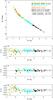 |
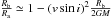
Fig. 3 Relation between visual surface brightness SV as a function of the color index (V − K)0. The black, light blue, green, brown, and red measurements are from Di Benedetto (2005), Boyajian et al. (2012), Hanbury Brown et al. (1974a), Maestro et al. (2013), and VEGA (this work), respectively. The red line corresponds to our fit when considering all stars. The rms of the difference between the surface brightness computed from our fit and measured surface brightness is presented in the lower panels (see the text for more detail). |
4.2. A revised SBC relation for late- and early-type stars
Historically, the SBC was first derived from interferometric observations of 18 stars by Wesselink (1969) using the (B − V) index. Five years later, the apparent angular diameters of 32 stars in the spectral range O5 to F8 have been measured using the NSII (Hanbury Brown et al. 1974a). Based on this sample, Barnes et al. (1976) and Barnes & Evans (1976) calibrated the SBC for late-type and early-type stars, respectively, but this was not done with the V − K color index. In order to constrain the SBC relation as a function of V − K we therefore use these 32 angular diameters (but 6 are rejected, see below). This is the first set of data we have used. We emphasize that the (V − K)0 color index is usually used to calibrated the SBC relation because it provides the lowest rms and it is mostly parallel to the reddening vector on the Sv − (V − K) diagram. Moreover, for all the datasets we have considered, we have recalculated the (V − K)0 and AV values in a similar way as for the VEGA objects (see Sect. 4.1).
More than ten years later, Di Benedetto (1998) made a careful compilation of 22 stars (with A, F, G, K spectral types) for which angular diameters were available in the literature and calibrated the SBC relation. Moreover, the direct application of the SBC relation to Cepheids was done by Fouque & Gieren (1997) and Di Benedetto (1998). Later, 27 stars were measured by NPOI and Mark III optical interferometers and the derived high precision angular diameters were published by Nordgren et al. (2001) and Mozurkewich et al. (2003), respectively. Finally, using a compilation of 29 dwarfs and subgiant (including the sun) in the 0.0 ≤ (V − K)0 ≤ 6.0 color range, Kervella et al. (2004) calibrated for the first time a linear SBC relation with an intrinsic dispersion of 0.02 mag or 1% in terms of angular diameter. A short time later, Di Benedetto (2005) made the same kind of compilation but with 45 stars in the − 0.1 ≤ (V − K)0 ≤ 3.7 color range (accuracy of 0.04 mag or 2% in terms of angular diameter). We use this larger second data set for our analysis.
One year later, Bonneau et al. (2006) provided a SBC relation (as function of V − K color magnitude) based on interferometric measurements, lunar occultation, and eclipsing binaries. We compare our results with those of Bonneau et al. (2006) and also Di Benedetto (2005) in Sect. 5.
Recently, Boyajian et al. (2012) enlarged the sample to 44 main-sequence A-, F-, and G-type stars using CHARA array measurements. In addition, ten stars with spectral types from B2 to F6 were observed using the astronomical visible observations (PAVO) beam combiner at the CHARA array (Maestro et al. 2013) and these recent CHARA measurements have been incorporated in our analysis.
However, in order to derive a SBC relation accurate enough for distance determination, one has to perform a consistent selection. Our strategy is the following: we consider all stars in multiple systems (as soon as the companion is far and faint enough not to contaminate interferometric measurements), fast rotators, and single stars. Fast rotating stars should be included as they improve the statistics of the relation (in particular for early-type objects), even if a slight bias is not excluded as discussed in Sect. 3.2 (see also next section). Conversely, we exclude stars with environments (like Be stars with strong wind) or stars with a strong variability. Following these criteria, we found seven stars to reject. The first one is Zeta Orionis (ζ Ori). Its angular diameter, measured by Hanbury Brown et al. (1974a) is most probably biased by a companion which was discovered later and with a separation of 40 mas (Hummel et al. 2000, 2013). Kappa Orionis (κ Ori) shows a P Cygni profile in Hα caused by a stellar wind (Searle et al. 2008; Stalio et al. 1981; Cassinelli et al. 1983). Delta Scorpii (δ Sco) is an active binary star exhibiting the Be phenomenon (Meilland et al. 2013). Gamma2 Velorum (γ2 Vel) is a binary system with a large spectral contribution from the Wolf-Rayet star (Millour et al. 2007). Zeta Ophiuchi (ζ Oph) is a magnetic star of Oe-type (Hubrig et al. 2011). Alpha Virginis (α Vir) is a double-lined spectroscopic binary (B1V+B4V) with an ellipsoidal variation of 0.03 mag due to tidal distortion (Harrington et al. 2009). The last one, Zeta Cassiopeiae (ζ Cas), is in the PAVO sample (Maestro et al. 2013). It stands at 7σ from the relation. It is a β Cepheid and the photometric contamination by a surrounding environment and/or a close companion is not excluded (Sadsaoud et al. 1994; Nardetto et al. 2011).
We finally end with 26 stars from Hanbury Brown et al.
(1974a), 44 stars from Boyajian et al.
(2012), 9 stars from Maestro et al.
(2013), and 45 values of Sv from Di Benedetto (2005), to which we can add our eight
angular diameters obtained with VEGA/CHARA. The total sample is composed of 132 stars
(with − 0.876 < V −
K < 3.69), including 32 early-type stars with
− 1 < V −
K < 0. Using this sample of 132 stars, we find
the relation 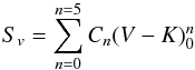 (10)with, C0 = 2.624 ±
0.009, C1 = 1.798 ± 0.020, C2 = − 0.776 ±
0.034, C3 = 0.517 ± 0.036, C4 = − 0.150 ±
0.015, and C5 = 0.015 ± 0.002. Uncertainties on
coefficients of the SBC relation do not take into account the X-axis uncertainties on
(V −
K)0. This relation can be used
consistently in the range − 0.9 ≤
V − K ≤ 3.7 with σSv =
0.10 mag. This corresponds to a relative precision on the angular
diameter of
(10)with, C0 = 2.624 ±
0.009, C1 = 1.798 ± 0.020, C2 = − 0.776 ±
0.034, C3 = 0.517 ± 0.036, C4 = − 0.150 ±
0.015, and C5 = 0.015 ± 0.002. Uncertainties on
coefficients of the SBC relation do not take into account the X-axis uncertainties on
(V −
K)0. This relation can be used
consistently in the range − 0.9 ≤
V − K ≤ 3.7 with σSv =
0.10 mag. This corresponds to a relative precision on the angular
diameter of 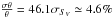 derived from Eq. (5) of Di Benedetto (2005). For stars earlier than A3
(− 0.9 < V −
K < 0.0), we successfully reached a magnitude
precision of σ =
0.16 or 7.3% in terms of angular diameter.
derived from Eq. (5) of Di Benedetto (2005). For stars earlier than A3
(− 0.9 < V −
K < 0.0), we successfully reached a magnitude
precision of σ =
0.16 or 7.3% in terms of angular diameter.
5. Discussion
Figure 3a shows the resulting SB relation as a function of the (V − K)0 color index for the five different data sets we have considered. The VEGA data appear in red in the figure. The residual O−Cv, which is the difference obtained between the measured surface brightness (O) and the relation provided by Eq. (10) (Cv), is shown in Fig. 3b. In the following, we define σ+ and σ− as the positive and negative standard deviation. We obtain σ+ = 0.07 and σ− = 0.09 for 0 < V − K < 3.7 (late-type stars, dot-dashed line in the figure) and σ+ = 0.13 mag and σ− = 0.18 mag for − 0.9 < V − K < 0 (early-type stars, dotted line in the figure). In Fig. 3c we derive the residual compared to the Di Benedetto (2005) relation (Eq. (2)) which is applicable only in the −0.1 < V − K < 4 color domain. We obtain a residual (O−Cd) which are similar: σ+ = 0.08 mag and σ− = 0.07 mag. This basically means that improving the statistics does not improve the thinnest of the relations. For this purpose, a homogeneous set of V and K photometry is probably required.
We also compare our results with those of Bonneau et al.
(2006), which is, to our knowledge, the only SBC relation, versus V − K,
provided for early-type stars in the literature (actually the relation is set from
−1.1 to 7, their Table 2), but
instead of using Eq. (2), they considered
another quantity,  . We therefore made a conversion to compare
with the SV quantity. The
residual (O−Cb) is shown in
Fig. 3d. We find σ+ = 0.10 mag and
σ− =
0.11 mag for 0 <
V − K < 4 (or late-type stars) and
σ+ =
0.23 mag and σ− = −0.23 mag for − 1 < V − K <
0 (or early-type stars). These residuals are significantly larger then
the ones obtained when using our Eq. (10) or
Eq. (2) from Di Benedetto (2005).
. We therefore made a conversion to compare
with the SV quantity. The
residual (O−Cb) is shown in
Fig. 3d. We find σ+ = 0.10 mag and
σ− =
0.11 mag for 0 <
V − K < 4 (or late-type stars) and
σ+ =
0.23 mag and σ− = −0.23 mag for − 1 < V − K <
0 (or early-type stars). These residuals are significantly larger then
the ones obtained when using our Eq. (10) or
Eq. (2) from Di Benedetto (2005).
In Fig. 3a we also have indicated the fast rotating stars and binaries. In Fig. 4 we provide a zoom of the SBC relation over the −1 < V − K < 0.25 color range. In this zoom we have also indicated the uncertainties and the names of the stars in our VEGA sample. We find that the O−Cv residual in the (V − K) color range −1 to 0 is σ = 0.06, σ = 0.17, and σ = 0.18, for stars in binary systems (6), for fast rotating stars (8), and for single stars (18). We note the following points:
First, we want to emphasize that a careful selection (by rejected stars with environment and stars with companions in contact), in particular in the range of −1 < V − K < 0 can significantly improve the precision on the SBC relation. We obtain σ ≃ 0.4 otherwise.
Second, the dispersion of the O−C residual for stars in binary systems is significantly lower (0.06) than to the one obtained with the whole sample (about 0.16), which indicates that interferometric and photometric measurements are not contaminated by the binarity.
Third, we obtain a large dispersion (σ = 0.17) for fast rotating stars. Five stars are beyond 1σ, while three are within, including ζ Peg in our VEGA sample (see Fig. 3b). Delta Cygni (δ Cyg) is, in particular, at 2σ. In Sect. 3.2, we estimated the impact of the fast rotation on the angular diameters of ζ Peg and δ Cyg to be 0.039 mas and 0.047 mas, respectively. Using Eq. (2), it translates into a magnitude effect of ± 0.150 mag and ± 0.127 mag, respectively. As already said, fast rotation modifies several stellar properties such as the shape of the photosphere (Collins 1963; Collins & Harrington 1966) and its brightness distribution (von Zeipel 1924a,b), which should be taken into consideration. However, studying these effects requires dedicated modeling, and this will be done in a forthcoming paper. Finally, in our VEGA sample, four stars are beyond 1σ from the relation, but when also considering the uncertainty in V − K, they remain consistent with the relation (see Fig. 4).
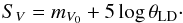
Fourth, we calculate the SBC relation for luminosity classes I and II, III, IV, and V (Fig.
5). We obtain the following results:
![Mathematical equation: \begin{eqnarray} &&-0.88\leq(V-K)_{0}\leq3.21 \nonumber\\ &&S_{v}=2.291 + 2.151(V-K)_{0} - 0.461(V-K)^{2}_{0} + 0.073(V-K)^{3}_{0} \nonumber\\ &&\left[\sigma_{S_{v}}=0.08~\mathrm{mag};\sigma_{\theta} \simeq 3.5\%; 12~\mathrm{stars; Class~I+II} \right] \\ \nonumber\\ &&-0.74\leq(V-K)_{0}\leq3.69 \nonumber\\ && S_{v}=2.497 + 1.916(V-K)_{0} -0.335(V-K)^{2}_{0} + 0.050(V-K)^{3}_{0}\nonumber\\ && \left[\sigma_{S_{v}}=0.07~\mathrm{mag};\sigma_{\theta} \simeq 3.4\%; 41~\mathrm{stars; Class~III} \right]\\ \nonumber \\ &&-0.58\leq(V-K)_{0}\leq2.06 \nonumber\\ &&S_{v}=2.625 + 1.823(V-K)_{0} -0.606(V-K)^{2}_{0} + 0.197(V-K)^{3}_{0}\nonumber\\ &&\left[\sigma_{S_{v}}=0.10~\mathrm{mag};\sigma_{\theta} \simeq 4.8\%; 79~\mathrm{stars; Class~IV+V} \right]\cdot \end{eqnarray}](/articles/aa/full_html/2014/10/aa23772-14/aa23772-14-eq305.png) We find a slight difference in the zero-points
of these relations. Their dispersion is, however, similar, about 0.09 mag, which is slightly
lower than the global dispersion of 0.16 mag that we obtain when considering the whole
sample.
We find a slight difference in the zero-points
of these relations. Their dispersion is, however, similar, about 0.09 mag, which is slightly
lower than the global dispersion of 0.16 mag that we obtain when considering the whole
sample.
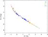 |
Fig. 5 Relation between the visual surface brightness SV and the color index (V − K)0 for luminosity class I (⋄), luminosity class II (∗), luminosity class III (×), luminosity class IV (△), and luminosity class V (°). |
6. Conclusions
Taking advantage of the unique VEGA/CHARA capabilities in terms of spatial resolution, we determined the angular diameters of eight bright early-type stars in the visible with a precision of about 1.5%. By combining these data with previous angular diameter determinations, we provide for the very first time a SBC relation for early-type stars with a precision of about 0.16 mag, which means that this SBC relation can be used to derive the angular diameter of early-type stars with a precision of 7.3%. This relation is a powerful tool for the distance scale calibration as it can be used to derive the individual angular diameters of detached, early-type, and thus bright eclipsing binary systems. It will be used in the course of the Araucaria Project (Gieren et al. 2005) to derive the distance of different galaxies in the Local Group, for exemple M33. As the eclipsing binary method is independent of the metallicity of the star, it can be used as a reference to test the impact of the metallicity on several other distance indicators, in particular the Cepheids. In the course of the Araucaria project, we also aim to test the method consistently on galactic early-type eclipsing binaries using photometry, spectroscopy, and interferometry.
Online material
Appendix A
Journal of the observations.
Available at http://www.jmmc.fr/searchcal
Available at http://www.jmmc.fr/litpro
Acknowledgments
This research has made use of the SIMBAD and VIZIER databases at the CDS (http://cdsweb.u- strasbg.fr/), Strasbourg (France), of the Jean-Marie Mariotti Center Aspro service (http://www.jmmc.fr/aspro), and of the electronic bibliography maintained by the NASA/ADS system. The research leading to these results has received funding from the European Community’s Seventh Framework Programme under Grant Agreement 312430 and financial support from the Ministry of Higher Education and Scientific Research (MHESR) − Tunisia. The CHARA Array is funded by the National Science Foundation through NSF grants AST-0606958 and AST-0908253 and by Georgia State University through the College of Arts and Sciences, as well as the W. M. Keck Foundation. W.G. gratefully acknowledges financial support for this work from the BASAL Centro de Astrofisica y Tecnologias Afines (CATA) PFB-06/2007, and from the Millenium Institute of Astrophysics (MAS) of the Iniciativa Cientifica Milenio del Ministerio de Economia, Fomento y Turismo de Chile, project IC120009. We acknowledge financial support for this work from ECOS-CONICYT grant C13U01. Support from the Polish National Science Center grant MAESTRO 2012/06/A/ST9/00269 is also acknowledged. We also wish to thank the referee, Dr Puls, for his numerous and precise suggestions for improving the photometric aspects of the paper. This was an enormous help in refining our results. This research has largely benefited from the support, suggestions, advice of our colleague Olivier Chesneau, who passed away this spring. The whole team wish to pay homage to him.
References
- Abt, H. A., & Morrell, N. I. 1995, ApJS, 99, 135 [Google Scholar]
- Abt, H. A., Levato, H., & Grosso, M. 2002, ApJ, 573, 359 [NASA ADS] [CrossRef] [Google Scholar]
- Allen de Prieto, C., & Lambert, D. L. 1999, A&A, 352, 555 [NASA ADS] [Google Scholar]
- Barnes, T. G., & Evans, D. S. 1976, MNRAS, 174, 489 [NASA ADS] [CrossRef] [Google Scholar]
- Barnes, T. G., Evans, D. S., & Parsons, S. B. 1976, MNRAS, 174, 503 [NASA ADS] [CrossRef] [Google Scholar]
- Blackwell, D. E., Petford, A. D., Arribas, S., Haddock, D. J., & Selby, M. J. 1990, A&A, 232, 396 [NASA ADS] [Google Scholar]
- Bohm-Vitense, E. 1985, ApJ, 296, 169 [NASA ADS] [CrossRef] [Google Scholar]
- Bonanos, A. Z., Stanek, K. Z., Kudritzki, R. P., et al. 2006, ApJ, 652, 313 [NASA ADS] [CrossRef] [Google Scholar]
- Bonneau, D., Clausse, J.-M., Delfosse, X., et al. 2006, A&A, 456, 789 [NASA ADS] [CrossRef] [EDP Sciences] [Google Scholar]
- Boyajian, T. S., McAlister, H. A., van Belle, G., et al. 2012, ApJ, 746, 101 [NASA ADS] [CrossRef] [Google Scholar]
- Cardelli, J. A., Clayton, G. C., & Mathis, J. S. 1989, ApJ, 345, 245 [NASA ADS] [CrossRef] [Google Scholar]
- Carpenter, K. G., Slettebak, A., & Sonneborn, G. 1984, ApJ, 286, 741 [CrossRef] [Google Scholar]
- Cassinelli, J. P., Myers, R. V., Hartmann, L., Dupree, A. K., & Sanders, W. T. 1983, ApJ, 268, 205 [NASA ADS] [CrossRef] [Google Scholar]
- Claret, A., & Bloemen, S. 2011, A&A, 529, A75 [NASA ADS] [CrossRef] [EDP Sciences] [Google Scholar]
- Collins, II, G. W. 1963, ApJ, 138, 1134 [NASA ADS] [CrossRef] [Google Scholar]
- Collins, II, G. W., & Harrington, J. P. 1966, ApJ, 146, 152 [NASA ADS] [CrossRef] [Google Scholar]
- Di Benedetto, G. P. 1998, A&A, 339, 858 [NASA ADS] [Google Scholar]
- Di Benedetto, G. P. 2005, MNRAS, 357, 174 [NASA ADS] [CrossRef] [Google Scholar]
- Ducati, J. R. 2002, VizieR Online Data Catalog: II/237 [Google Scholar]
- Evans, N. R. 1991, ApJ, 372, 597 [NASA ADS] [CrossRef] [Google Scholar]
- Evans, N. R. 1992, ApJ, 389, 657 [NASA ADS] [CrossRef] [Google Scholar]
- Feast, M. W. 1997, MNRAS, 284, 761 [NASA ADS] [CrossRef] [Google Scholar]
- Fitzpatrick, E. L. 1999, PASP, 111, 63 [NASA ADS] [CrossRef] [Google Scholar]
- Fitzpatrick, E. L., & Massa, D. 2005, AJ, 129, 1642 [NASA ADS] [CrossRef] [EDP Sciences] [Google Scholar]
- Fouque, P., & Gieren, W. P. 1997, A&A, 320, 799 [NASA ADS] [Google Scholar]
- Freedman, W. L., & Madore, B. F. 1996, in Clusters, Lensing, and the Future of the Universe, eds. V. Trimble, & A. Reisenegger, ASP Conf. Ser., 88, 9 [Google Scholar]
- Freedman, W. L., Madore, B. F., Rigby, J., Persson, S. E., & Sturch, L. 2008, ApJ, 679, 71 [NASA ADS] [CrossRef] [Google Scholar]
- Gieren, W., Pietrzyński, G., Soszyński, I., et al. 2005, ApJ, 628, 695 [NASA ADS] [CrossRef] [Google Scholar]
- Gies, D. R., & Lambert, D. L. 1992, ApJ, 387, 673 [NASA ADS] [CrossRef] [Google Scholar]
- Graczyk, D., Soszyński, I., Poleski, R., et al. 2011, Acta Astron., 61, 103 [NASA ADS] [Google Scholar]
- Graczyk, D., Pietrzyński, G., Thompson, I. B., et al. 2012, ApJ, 750, 144 [NASA ADS] [CrossRef] [Google Scholar]
- Graczyk, D., Pietrzyński, G., Thompson, I. B., et al. 2014, ApJ, 780, 59 [NASA ADS] [CrossRef] [Google Scholar]
- Gray, D. F. 1980, PASP, 92, 771 [NASA ADS] [CrossRef] [Google Scholar]
- Hanbury Brown, R., Davis, J., & Allen, L. R. 1974a, MNRAS, 167, 121 [NASA ADS] [CrossRef] [Google Scholar]
- Hanbury Brown, R., Davis, J., Lake, R. J. W., & Thompson, R. J. 1974b, MNRAS, 167, 475 [NASA ADS] [CrossRef] [Google Scholar]
- Harrington, D., Koenigsberger, G., Moreno, E., & Kuhn, J. 2009, ApJ, 704, 813 [NASA ADS] [CrossRef] [Google Scholar]
- Hauschildt, P. H., Baron, E., & Allard, F. 1997, ApJ, 483, 390 [NASA ADS] [CrossRef] [Google Scholar]
- Hohle, M. M., Neuhäuser, R., & Schutz, B. F. 2010, Astron. Nachr., 331, 349 [NASA ADS] [CrossRef] [Google Scholar]
- Hubrig, S., Oskinova, L. M., & Schöller, M. 2011, Astron. Nachr., 332, 147 [NASA ADS] [CrossRef] [Google Scholar]
- Hummel, C. A., White, N. M., Elias, II, N. M., Hajian, A. R., & Nordgren, T. E. 2000, ApJ, 540, L91 [NASA ADS] [CrossRef] [Google Scholar]
- Hummel, C. A., Rivinius, T., Nieva, M.-F., et al. 2013, A&A, 554, A52 [NASA ADS] [CrossRef] [EDP Sciences] [Google Scholar]
- Johnson, H. L., & Morgan, W. W. 1953, ApJ, 117, 313 [NASA ADS] [CrossRef] [Google Scholar]
- Johnson, H. L., Mitchell, R. I., Iriarte, B., & Wisniewski, W. Z. 1966, Communications of the Lunar and Planetary Laboratory, 4, 99 [Google Scholar]
- Kervella, P., Thévenin, F., Di Folco, E., & Ségransan, D. 2004, A&A, 426, 297 [NASA ADS] [CrossRef] [EDP Sciences] [Google Scholar]
- Kurucz, R. L. 1970, SAO Special Report, 309 [Google Scholar]
- Laney, C. D., & Stobie, R. S. 1993, MNRAS, 263, 921 [Google Scholar]
- Laney, C. D., Joner, M. D., & Pietrzyński, G. 2012, MNRAS, 419, 1637 [NASA ADS] [CrossRef] [Google Scholar]
- Lyubimkov, L. S., Rachkovskaya, T. M., Rostopchin, S. I., & Lambert, D. L. 2002, MNRAS, 333, 9 [NASA ADS] [CrossRef] [Google Scholar]
- Macri, L. M., Stanek, K. Z., Sasselov, D. D., Krockenberger, M., & Kaluzny, J. 2001, AJ, 121, 870 [NASA ADS] [CrossRef] [Google Scholar]
- Maestro, V., Che, X., Huber, D., et al. 2013, MNRAS, 434, 1321 [NASA ADS] [CrossRef] [Google Scholar]
- Massey, P., Neugent, K. F., Hillier, D. J., & Puls, J. 2013, ApJ, 768, 6 [NASA ADS] [CrossRef] [Google Scholar]
- McDonald, I., Zijlstra, A. A., & Boyer, M. L. 2012, MNRAS, 427, 343 [NASA ADS] [CrossRef] [Google Scholar]
- Meilland, A., Stee, P., Spang, A., et al. 2013, A&A, 550, L5 [NASA ADS] [CrossRef] [EDP Sciences] [Google Scholar]
- Mermilliod, J.-C., Mermilliod, M., & Hauck, B. 1997, A&AS, 124, 349 [NASA ADS] [CrossRef] [EDP Sciences] [Google Scholar]
- Millour, F., Petrov, R. G., Chesneau, O., et al. 2007, A&A, 464, 107 [NASA ADS] [CrossRef] [EDP Sciences] [Google Scholar]
- Mochejska, B. J., Kaluzny, J., Stanek, K. Z., & Sasselov, D. D. 2001, AJ, 122, 1383 [NASA ADS] [CrossRef] [Google Scholar]
- Mourard, D., Clausse, J. M., Marcotto, A., et al. 2009, A&A, 508, 1073 [NASA ADS] [CrossRef] [EDP Sciences] [Google Scholar]
- Mourard, D., Bério, P., Perraut, K., et al. 2011, A&A, 531, A110 [NASA ADS] [CrossRef] [EDP Sciences] [Google Scholar]
- Mozurkewich, D., Armstrong, J. T., Hindsley, R. B., et al. 2003, AJ, 126, 2502 [NASA ADS] [CrossRef] [Google Scholar]
- Nardetto, N., Mourard, D., Tallon-Bosc, I., et al. 2011, A&A, 525, A67 [NASA ADS] [CrossRef] [EDP Sciences] [Google Scholar]
- Nordgren, T. E., Sudol, J. J., & Mozurkewich, D. 2001, AJ, 122, 2707 [NASA ADS] [CrossRef] [Google Scholar]
- Pasinetti Fracassini, L. E., Pastori, L., Covino, S., & Pozzi, A. 2001, A&A, 367, 521 [NASA ADS] [CrossRef] [EDP Sciences] [Google Scholar]
- Pawlak, M., Graczyk, D., Soszyński, I., et al. 2013, Acta Astron., 63, 323 [NASA ADS] [Google Scholar]
- Pecaut, M. J., & Mamajek, E. E. 2013, ApJS, 208, 9 [NASA ADS] [CrossRef] [Google Scholar]
- Pietrzyński, G., & Gieren, W. 2002, AJ, 124, 2633 [NASA ADS] [CrossRef] [Google Scholar]
- Pietrzyński, G., Gieren, W., Szewczyk, O., et al. 2008, AJ, 135, 1993 [NASA ADS] [CrossRef] [Google Scholar]
- Pietrzyński, G., Thompson, I. B., Graczyk, D., et al. 2009, ApJ, 697, 862 [NASA ADS] [CrossRef] [Google Scholar]
- Pietrzyński, G., Graczyk, D., Gieren, W., et al. 2013, Nature, 495, 76 [NASA ADS] [CrossRef] [PubMed] [Google Scholar]
- Sadsaoud, H., Le Contel, J. M., Chapellier, E., Le Contel, D., & Gonzalez-Bedolla, S. 1994, A&A, 287, 509 [NASA ADS] [Google Scholar]
- Searle, S. C., Prinja, R. K., Massa, D., & Ryans, R. 2008, A&A, 481, 777 [NASA ADS] [CrossRef] [EDP Sciences] [Google Scholar]
- Slettebak, A., Collins, II, G. W., Parkinson, T. D., Boyce, P. B., & White, N. M. 1975, ApJS, 29, 137 [NASA ADS] [CrossRef] [Google Scholar]
- Stalio, R., Sedmak, G., & Rusconi, L. 1981, A&A, 101, 168 [NASA ADS] [Google Scholar]
- Sturmann, J., ten Brummelaar, T., Sturmann, L., & McAlister, H. A. 2010, in SPIE Conf. Ser., 7734, 45 [Google Scholar]
- Szewczyk, O., Pietrzyński, G., Gieren, W., et al. 2008, AJ, 136, 272 [NASA ADS] [CrossRef] [Google Scholar]
- Tallon-Bosc, I., Tallon, M., Thiébaut, E., et al. 2008, SPIE, 7013 [Google Scholar]
- ten Brummelaar, T. A., McAlister, H. A., Ridgway, S. T., et al. 2005, ApJ, 628, 453 [NASA ADS] [CrossRef] [Google Scholar]
- Tetzlaff, N., Neuhäuser, R., & Hohle, M. M. 2011, MNRAS, 410, 190 [NASA ADS] [CrossRef] [Google Scholar]
- Torres, G., Andersen, J., & Giménez, A. 2010, A&ARv, 18, 67 [Google Scholar]
- Udalski, A., Pietrzyński, G., Woźniak, P., et al. 1998a, ApJ, 509, L25 [NASA ADS] [CrossRef] [Google Scholar]
- Udalski, A., Szymanski, M., Kubiak, M., et al. 1998b, Acta Astron., 48, 1 [Google Scholar]
- van Belle, G. T. 2012, A&ARv, 20, 51 [NASA ADS] [CrossRef] [Google Scholar]
- van Belle, G. T., Ciardi, D. R., Ten Brummelaar, T., et al. 2006, ApJ, 637, 494 [NASA ADS] [CrossRef] [Google Scholar]
- van Leeuwen, F. 2007, A&A, 474, 653 [NASA ADS] [CrossRef] [EDP Sciences] [Google Scholar]
- Vilardell, F., Ribas, I., & Jordi, C. 2006, A&A, 459, 321 [NASA ADS] [CrossRef] [EDP Sciences] [Google Scholar]
- von Zeipel, H. 1924a, MNRAS, 84, 665 [NASA ADS] [CrossRef] [Google Scholar]
- von Zeipel, H. 1924b, MNRAS, 84, 684 [NASA ADS] [CrossRef] [Google Scholar]
- Wegner, W. 1994, MNRAS, 270, 229 [NASA ADS] [CrossRef] [Google Scholar]
- Wesselink, A. J. 1969, MNRAS, 144, 297 [NASA ADS] [CrossRef] [Google Scholar]
- Wu, Y., Singh, H. P., Prugniel, P., Gupta, R., & Koleva, M. 2011, A&A, 525, A71 [NASA ADS] [CrossRef] [EDP Sciences] [Google Scholar]
- Wyrzykowski, L., Udalski, A., Kubiak, M., et al. 2003, Acta Astron., 53, 1 [NASA ADS] [CrossRef] [Google Scholar]
- Wyrzykowski, L., Udalski, A., Kubiak, M., et al. 2004, Acta Astron., 54, 1 [NASA ADS] [CrossRef] [Google Scholar]
- Zorec, J., & Royer, F. 2012, A&A, 537, A120 [NASA ADS] [CrossRef] [EDP Sciences] [Google Scholar]
- Zorec, J., Cidale, L., Arias, M. L., et al. 2009, A&A, 501, 297 [NASA ADS] [CrossRef] [EDP Sciences] [Google Scholar]
All Tables
Reference stars and their parameters, including the spectral type, the visual magnitude (mV), and the predicted uniform disk angular diameter (in mas) derived from the JMMC SearchCal software (Bonneau et al. 2006).
Angular diameters obtained with VEGA/CHARA and the corresponding surface brightness.
All Figures
|
Fig. 1 Time sequences of raw visibilities of the science observations (light blue dots), calibrated (blue dots) using the transfer function (red dots). |
| In the text | |
|
Fig. 2 Squared visibility versus spatial frequency for all stars in our sample with their corresponding statistical uncertainties. The red solid lines indicate the best uniform disk model obtained from the LITpro fitting software. |
| In the text | |
|
Fig. 3 Relation between visual surface brightness SV as a function of the color index (V − K)0. The black, light blue, green, brown, and red measurements are from Di Benedetto (2005), Boyajian et al. (2012), Hanbury Brown et al. (1974a), Maestro et al. (2013), and VEGA (this work), respectively. The red line corresponds to our fit when considering all stars. The rms of the difference between the surface brightness computed from our fit and measured surface brightness is presented in the lower panels (see the text for more detail). |
| In the text | |
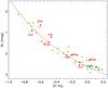 |
Fig. 4 Same as Fig.3, but with the names of the VEGA/CHARA stars in our sample (in red). |
| In the text | |
|
Fig. 5 Relation between the visual surface brightness SV and the color index (V − K)0 for luminosity class I (⋄), luminosity class II (∗), luminosity class III (×), luminosity class IV (△), and luminosity class V (°). |
| In the text | |
Current usage metrics show cumulative count of Article Views (full-text article views including HTML views, PDF and ePub downloads, according to the available data) and Abstracts Views on Vision4Press platform.
Data correspond to usage on the plateform after 2015. The current usage metrics is available 48-96 hours after online publication and is updated daily on week days.
Initial download of the metrics may take a while.