| Issue |
A&A
Volume 570, October 2014
|
|
|---|---|---|
| Article Number | A116 | |
| Number of page(s) | 15 | |
| Section | Stellar structure and evolution | |
| DOI | https://doi.org/10.1051/0004-6361/201423757 | |
| Published online | 31 October 2014 | |
Revealing the pulsational properties of the V777 Herculis star KUV 05134+2605 by its long-term monitoring⋆
1 Konkoly Observatory, MTA CSFK, Konkoly Thege M. u. 15-17, 1121 Budapest, Hungary
e-mail: This email address is being protected from spambots. You need JavaScript enabled to view it.
2 Facultad de Ciencias Astronómicas y Geofísicas, Universidad Nacional de La Plata, Argentina
3 Consejo Nacional de Investigaciones Científicas y Ténicas (CONICET), Argentina
4 Instituto de Física, Universidade Federal do Rio Grande do Sul, 91501-900 Porto-Alegre, RS, Brazil
5 Department of Astronomy, Eötvös Loránd University, Pázmány Péter sétány 1/A, 1117 Budapest, Hungary
Received: 4 March 2014
Accepted: 11 August 2014
Abstract
Context. KUV 05134+2605 is one of the 21 pulsating DB white dwarfs (V777 Her or DBV variables) known so far. The detailed investigation of the short-period and low-amplitude pulsations of these relatively faint targets requires considerable observational efforts from the ground, long-term single-site or multi-site observations. The observed amplitudes of excited modes undergo short-term variations in many cases, which makes determining pulsation modes difficult.
Aims. We aim to determine the pulsation frequencies of KUV 05134+2605, find regularities between the frequency and period components, and perform an asteroseismic investigation for the first time.
Methods. We re-analysed the published data and collected new measurements. We compared the frequency content of the different datasets from the different epochs and performed various tests to check the reliability of the frequency determinations. The mean period spacings were investigated with linear fits to the observed periods, Kolmogorov-Smirnov and inverse variance significance tests, and with a Fourier analysis of different period sets, including a Monte Carlo test that simulated the effect of alias ambiguities. We employed fully evolutionary DB white dwarf models for the asteroseismic investigations.
Results. We identified 22 frequencies between 1280 and 2530 μHz. These form 12 groups, which suggests at least 12 possible frequencies for the asteroseismic investigations. Thanks to the extended observations, KUV 05134+2605 joined the group of rich white dwarf pulsators. We identified one triplet and at least one doublet with a ≈ 9 μHz frequency separation, from which we derived a stellar rotation period of 0.6 d. We determined the mean period spacings of ≈ 31 s and 18 s for the modes we propose as dipole and quadrupole. We found an excellent agreement between the stellar mass derived from the ℓ = 1 period spacing and the period-to-period fits, all providing M∗ = 0.84 − 0.85 M⊙ solutions. Our study suggests that KUV 05134+2605 is the most massive amongst the known V777 Her stars.
Key words: techniques: photometric / stars: individual: KUV 05134+2605 / stars: interiors / stars: oscillations / white dwarfs
Tables of the photometric time series are only available at the CDS via anonymous ftp to cdsarc.u-strasbg.fr (130.79.128.5) or via http://cdsarc.u-strasbg.fr/viz-bin/qcat?J/A+A/570/A116
© ESO, 2014
1. Introduction
The discovery of the first pulsating DB-type white dwarf (GD 358 or V777 Her) was not serendipitous: it was the result of a dedicated search for unstable modes in these stars, driven by the partial ionization of the atmospheric helium (Winget et al. 1982).
The V777 Her stars are similar to their “cousins”, the ZZ Ceti (or DAV) stars, in their pulsational properties. Both show light variations caused by non-radial g-mode pulsations with periods between 100−1400 s. However, the V777 Her stars have higher effective temperatures (22 000−29 000 K) than the DAVs (10 900−12 300 K). Another significant difference is the composition of their atmospheres: hydrogen dominates the DAV, while helium constitutes the DBV atmospheres. The classification of the recently discovered cool (Teff ~ 8000−9000 K), extremely low-mass pulsating DA white dwarfs as ZZ Ceti stars was proposed by the modelling results of Van Grootel et al. (2013). However, except for their similar driving mechanism and surface composition, they are completely different: they likely have a binary origin, their cores are dominated by helium, and they pulsate with longer periods associated to g-modes than the ZZ Ceti stars (Hermes et al. 2013). About 80% of the white dwarfs belong to the DA spectral class (e.g. Kleinman et al. 2013) and most of the known white dwarf pulsators are ZZ Ceti variables. With the discovery of pulsations in KIC 8626021, there are still only 21 known V777 Her stars (Østensen et al. 2011).
The regularities between the observed frequencies and periods offer great potential for asteroseismic investigations of pulsating white dwarfs. Theoretically, rotational splitting of dipole and quadrupole modes into three or five equally spaced components allows determining the stellar rotation period, but the internal differential rotation (Kawaler et al. 1999) and the magnetic field (Jones et al. 1989) can complicate this picture. These rotationally split frequencies can also be hard to detect: we need a long enough dataset to resolve the components, the overlapping splitting structures of the closely spaced modes can make the finding of the regularities difficult, and the frequency separations can be close to the daily alias of ground-based measurements. Furthermore, observational results indicate that in many cases not all of the components reach an observable amplitude at a given time, for unknown reasons (Winget & Kepler 2008).
The other theoretically predicted regularity is the quasi equally spaced formation of the consecutive radial overtone pulsation periods of the same spherical harmonic index (ℓ). The inner chemical stratification breaks the uniform spacings, while the mean period spacing is an indicator of the total stellar mass.
The typical feature of the white dwarf pulsation is that the light curves are not sinusoidal, and we can detect combination (nfi ± mfj), harmonic (nfi), or even subharmonic (n/ 2fi) peaks in the corresponding Fourier transforms. These features reveal the importance of the non-linear effects on the observed light variations.
For more details on the general properties of white dwarf pulsators, we refer to the reviews of Winget & Kepler (2008), Fontaine & Brassard (2008), and Althaus et al. (2010).
The pulsation frequencies of V777 Her stars are reported to undergo short-term amplitude and phase variations (see e.g. Handler et al. 2003 and 2002). The most famous example is the so-called sforzando effect observed in GD 358. This star showed a high-amplitude sinusoidal light variation for a short period of time instead of the non-linear variability observed just a day before (Kepler et al. 2003; Provencal et al. 2009). To explain the short-term changes in the pulsational behaviour of a star is challenging. Because convection plays an important role in driving the pulsations, interactions of pulsation and convection might explain some of the temporal variations (Montgomery et al. 2010). For the pre-white dwarf GW Vir pulsator PG 0122+200, Vauclair et al. (2011) found that the temporal variations of pulsation modes may be the result of resonant coupling induced by rotation within triplets. In some cases, observed amplitude variations are the result of the insufficient frequency resolution of the datasets, and do not reflect real changes in the frequencies’ energy content.
We assume that the structure of a star, which determines which pulsation frequencies can be excited, does not change on time-scales as short as the number of detectable frequencies and their amplitudes in many white dwarfs. As a consequence of amplitude variations, one dataset reveals only a subset of the possible frequencies, but with observations at different epochs, we can add more and more frequencies to the list of observed ones, which is essential for asteroseismic investigations (see e.g. the pioneer case of G29-38 reported by Kleinman et al. 1998). Here, observations of KUV 05134+2605 at different epochs provide a more complete sampling of the pulsation frequencies, which will then lead to a more detailed asteroseismic analysis.
Asteroseismology can provide information on the masses of the envelope layers, the core structure, and the stellar mass. These are crucial for building more realistic models and improving our knowledge of stellar evolution. More than 95% of the stars will end their life as white dwarfs and the information we gather on pulsating members is representative of the non-pulsating ones because most, if not all, stars pulsate when they cross the instability strip. Therefore asteroseismic studies of DAVs and DBVs provide important constraints on our models of stellar evolution and galactic history.
For KUV 05134+2605, previous observations suggested a rich amplitude spectrum showing considerable amplitude variations from season to season (Handler et al. 2003). This made the star a promising target for additional monitoring. Our main goal was to find the excited normal modes with data obtained in different seasons. In this paper, we discuss our findings and the results on the asteroseismic investigations based on the set of pulsation modes.
2. Observations and data reduction
The first detection of the light variations of KUV 05134+2605 (V = 16.3 mag, α2000 = 05h16m28s, δ2000 = + 26d08m38s) was announced by Grauer et al. (1989). Later, several multi- and single-site observations followed the discovery run. Data were collected in 1992, 2000, and 2001, including the Whole Earth Telescope (WET, Nather et al. 1990) run in 2000 November (XCov20), when KUV 05134+2605 was one of the secondary targets. In this paper, we re-analyse these datasets. The log of observations and the reduction process applied in these cases are summarized in Handler et al. (2003).
To complement the earlier measurements, we collected data on KUV 05134+2605 on 11 nights in the 2007/2008 observing season with the 1m Ritchey-Chrétien-Coudé telescope at Piszkéstető mountain station of Konkoly Observatory. We continued the observations in 2011 for three nights. The measurements were made with a Princeton Instruments VersArray:1300B back-illuminated CCD camera in white light and with 30 s integration times. Table 1 shows the journal of the Konkoly observations. We obtained ≈ 48 and 7 h of data in 2007/2008 and 2011.
Log of observations of KUV 05134+2605, performed at Piszkéstető, Konkoly Observatory.
We followed the standard reduction procedure of the raw data frames: we applied bias, dark and flat corrections, and performed aperture photometry of the variable and comparison stars, using standard IRAF1 routines. We converted the Julian date (JD) times to barycentric JDs in barycentric dynamical time (BJDTDB) using the applet of Eastman et al. (2010)2. After the aperture photometry, we verified that the light curves of the possible comparison stars were free from any instrumental effects or variability. Finally, we selected three stars and used their average brightness as a comparison for the differential photometry. Figure 1 shows the variable and the comparisons in the CCD field. We corrected for the atmospheric extinction and for the instrumental trends by applying low-order polynomial fits to the resulting light curves. This affected the low-frequency region in the Fourier transforms (FTs) below 350 μHz. Therefore we did not investigate this frequency domain. Figure 2 presents the light curves from the 2007/2008 and 2011 seasons. The Rayleigh frequency resolutions (1 / ΔT) of the light curves for these two epochs are 0.1 and 2.3 μHz.
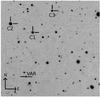 |
Fig. 1 One of the CCD frames obtained at Piszkéstető, Konkoly Observatory, with the variable and comparison stars marked. The field of view is ≈ 7′ × 7′. |
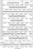 |
Fig. 2 Normalized differential light curves of the Konkoly runs. Data were collected in the 2007/2008 observing season (upper panels) and in 2011 (lower panels). For better visibility of the pulsation cycles, we connected the points with grey lines. Boldface numbers in the corners correspond to the run numbers in Table 1. |
The most important parameters of the individual datasets used in this study can be found in Table 2. This way, we can compare the different runs quantitatively, which can also be useful in interpreting their frequency content.
3. Frequency content of the datasets
We performed a Fourier analysis of the datasets using the program MuFrAn (Multi-Frequency Analyser, Kolláth 1990; Csubry & Kolláth 2004). This tool can handle gapped and unequally spaced data, has fast Fourier and discrete Fourier transform abilities, and is also capable of performing linear and non-linear fits of Fourier components. The results were also checked with PERIOD04 (Lenz & Breger 2005) and the photometry modules of FAMIAS (Zima 2008).
As Table 2 shows, the long time-base of the data obtained in the 2007/2008 season (hereafter Konkoly2007 data) and the WET data from 2000 (hereafter WET2000 data) provide the best Rayleigh frequency resolution and have the lowest noise levels. We review the results of the Fourier analyses of these two datasets first.
Comparison of the different observing runs on KUV 05134+2605.
3.1. Analysis of the WET2000 and Konkoly2007 data
Figure 3 presents the successive pre-whitening steps of the datasets. We checked not only the resulting amplitude, phase, and frequency values, but the significance of the peaks in every fit. We took into account the peaks that reached the 4 ⟨ A ⟩ level (dashed lines), calculated by the moving average of radius ~ 1000 μHz of the residual of the previous step’s FT.
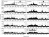 |
Fig. 3 Successive pre-whitening steps of the analyses of the WET2000 and Konkoly2007 datasets. The window functions are given in the insets. Dashed lines denote the 4 ⟨ A ⟩ significance levels calculated by the moving average of the spectra. |
The choice of the frequencies showing the highest amplitudes was not automatic during the pre-whitening process, as the 1 d-1 alias peaks have relatively large amplitudes (see the window functions inserted in Fig. 3). Thus, we fitted the data in different trials not only with the subsequent frequency with the highest amplitude, but also with its ±1−2 d-1 aliases instead, and compared the resulting FTs and the associated light-curve residual values (this represents the square root of the mean standard deviation between the fitted curve and the data). For the Konkoly2007 dataset, the results of data subsets’ Fourier analyses also helped to decide which frequency we considered as real. For the frequency determination tests, see Sect. 3.3.
The first columns of Table 3 summarize the pre-whitening results obtained on the WET2000 and Konkoly2007 data, showing the frequencies and amplitudes of the 9 and 13 peaks that exceed the 4 ⟨ A ⟩ significance level.
Results of the frequency analyses of the datasets from different observing seasons.
In the WET2000 dataset, we detect two closely spaced frequencies as dominant ones (at 1901.9 and 1892.3 μHz) with a 9.6 μHz frequency spacing (see the first two panels on the left of Fig. 3). The main pulsation frequency region is between ≈ 1200 and 2000 μHz.
The 1893.8 μHz frequency is close to a higher amplitude frequency (δf = 1.5 μHz, beat period: 7.5 d). We considered and investigated in Sect. 3.3 the possibility that this is not a real pulsation frequency, but represents an example for an artificial peak that emerges as a result of temporal amplitude variations.
Similarly to the WET2000 data, two closely spaced frequencies dominate the Konkoly2007 dataset, but at 1623.7 and 1614.5 μHz. The dominant frequencies of the WET2000 data are below the detection limit. An additional frequency can be detected at 1633.0 μHz in the Konkoly2007 data, which completes the dominant doublet into an almost exactly equidistant triplet with spacings of 9.2 and 9.3 μHz (and corresponding beat periods of 1.3 and 1.2 d). This is the only complete triplet structure detected in a single dataset.
In the Konkoly2007 data, we find a doublet around 1450 μHz in addition to the triplet, but with a different spacing: only 6.9 μHz. In the 1700 − 1900 μHz region there are many peaks, and identifying the real pulsation peaks is difficult. We consider the three-frequency solution, in which one of the frequencies, at 1831.0 μHz, can also be detected in a Konkoly2007 data subset (see Sect. 3.3). The other two frequencies at 1767.1 and 1800.5 μHz are the same within the uncertainties as the 1762.9 and 1798.6 μHz frequencies detected in the 2001 and WET2000 data, respectively.
The 2275.1 μHz frequency is also considerably close to a larger amplitude frequency at 2277.6 μHz, similarly to the 1893.8 μHz frequency of the WET2000 data.
The 3902.1 μHz frequency in the Konkoly2007 dataset is a combination (f1 + f2) of the two large-amplitude frequencies at 1623.7 and 2277.6 μHz. We did not detect other combination frequencies in the WET2000 or in the Konkoly2007 dataset.
In conclusion, we find a common frequency of the WET2000 and Konkoly2007 datasets at 1800 μHz. The frequencies at 1633.0 μHz (2007) and 1644.2 (2000) are also common, if we consider that these are most likely 1 d-1 (11.574 μHz) aliases.
The peaks found at 1681.7 and 1767.1 μHz (2007) are also slightly different from those detected at 1699.9 and 1781.7 μHz (2000). Different scenarios can explain the emergence of these frequency pairs (alias ambiguities, rotational splitting, the mixing of dipole and quadrupole modes). We discuss them in Sect. 3.4.
3.2. Analysis of the short datasets obtained between 1988 and 2011
Table 3 also summarizes the results of the Fourier analysis of the short light curves. The largest number of frequencies are detected in the 1988 and 1992 data (5−5 frequencies). In 2000, 2001, and 2011, two, one, and two frequencies exceeded the 4 ⟨ A ⟩ significance level, respectively. The dominant frequency, around 1901 μHz, did not change from 2000 October to 2000 November−December (WET2000), while it was different in all the other observing seasons.
1988: the 1287.6 and the 1504.5 μHz frequencies are candidates for new pulsation modes. The 1414.7 μHz frequency is close to the 2 d-1 alias of the 1390.6 μHz peak of the WET2000 dataset, but it could still be an independent frequency. The two frequencies above 2800 μHz can be interpreted as combination terms, considering the alias ambiguities.
1992: in the 1992 dataset, we detect a doublet at 1465.4 and 1474.5 μHz with 9.1 μHz separation. We note that this separation is slightly lower than the Rayleigh frequency resolution of the dataset (9.9 μHz). We checked the reliability of this doublet in the course of the frequency determination tests, see Sects. 3.3 and 3.4. The 1612.9 μHz frequency corresponds to the 1614.5 μHz frequency from 2007. The 2504.7 μHz frequency might be a −2 d-1 alias of the 2530.7 μHz frequency that was also detected in 2007, or might represent a new pulsation frequency.
2000: the two significant frequencies obtained in 2000 October correspond to the two largest amplitude frequencies detected in the WET2000 dataset.
2001: the only significant frequency of the 2001 data at 1762.9 μHz is the same within the uncertainties as the 1767.1 μHz frequency observed in 2007, which confirms the choice of the latter during the pre-whitening process.
2011: the 2023.7 μHz peak is a promising candidate for a new pulsation mode. The frequency at 1472 μHz was found in the 1992 data.
3.3. Frequency determination tests
We performed several different tests based both on observational and synthetic data to investigate the reliability of the frequency solutions presented in Table 3. These tests also help to calculate more realistic uncertainties for the frequency values than the simple formal uncertainties derived from the light-curve fits.
Analysis of data subsets: the Konkoly2007 dataset provides the longest time base, but it also has the poorest temporal coverage. We selected four data subsets for independent analysis: subset 1 (runs 3 and 4 in Table 1), subset 2 (runs 1 − 4), subset 3 (runs 6 − 8) and subset 4 (runs 9 − 11). Comparing to the result of the Fourier analysis of the whole dataset (Table 3), we found five frequencies that were also significant in the subset data. Four of them (at 1456, 1624, 1633, and 1831 μHz) were detected only once, but we found the 2277 μHz frequency in every subset.
Analysis of synthetic datasets: we performed this test separately for every dataset: the 1988, 1992, 2000 Oct., WET2000, 2001, Konkoly2007, Konkoly2011, and also the subset 1 − 4 data. In this step, we generated at least 50 synthetic light-curves with the same timings as the original data and with Gaussian random noise added, using the frequencies, amplitudes, and phases of the corresponding light-curve solution presented in Table 3. The applied noise level was calculated according to the residual scatter of the given light-curve solution. We carried out an independent and automated frequency analysis of each synthetic dataset with the program SigSpec (Reegen 2007). In this way we eliminated the subjective personal factor for instance in the selection of the starting frequency. We finally checked the percentage that the program found for the input frequencies instead of their aliases. The success rates we obtained for the different frequencies are between 34 and 100 percent, but above 70 percent in most cases.
Analysis of synthetic datasets with amplitude variations: temporal variations in pulsating white dwarfs are well known, and from comparing the FTs of different epoch datasets, the amplitude variations of KUV 05134+2605 are obvious. However, the Fourier analysis method we applied for the pre-whitening assumes constant amplitudes, frequencies, and phases for the pulsation. Any deviations from this assumption may result in the emergence of additional peaks in the Fourier spectrum.
We divided the Konkoly2007 dataset into five subsets: subset a, b, c, d, and e (runs 1–2, 3–4, 5, 6–8, and 9−11), and generated synthetic light-curves for the times of these subsets. We fixed the Konkoly2007 frequencies and phases according to those determined by the whole dataset, but let the amplitudes vary from subset to subset for every frequency. We omitted only the combination term at 3902.1 μHz and the 2275.1 μHz frequency from the test. This latter may be an artefact resulting from temporal variations in the pulsation, and we checked in this way whether amplitude changes can really cause such closely spaced peaks. We chose the amplitudes applied to represent both slight and major variations from subset to subset, based on the observed values. We constructed in this way a new, synthetic Konkoly2007 dataset with variable amplitudes. We then created 50 of these and added Gaussian random noise as in the case of the fixed-amplitude tests, and analysed them with SigSpec. The program found the original frequencies with 22–98 percent success rates, and 6 out of the 11 frequencies reached or exceeded the 70 percent rate.
The other finding is that amplitude variations can indeed cause the emergence of closely spaced low-amplitude peaks in the Fourier transforms. For example, the doublet at 2277.6 and 2278.5 μHz, which shows 3.9 mmag and 2.8 mmag amplitudes and a frequency separation of 0.9 μHz in one of the test datasets. Similarly closely spaced peaks were detected for example in the ZZ Ceti stars KUV 02464+3239 (Bognár et al. 2009) and EC14012-1446 (Provencal et al. 2012). Both stars show variable amplitudes on a time scale of weeks.
3.3.1. Conclusions
The main goal of these tests was to investigate the robustness of the light-curve solutions presented in Table 3. Based on the results, we constructed the list of frequencies considered as real (see Table 4) by applying the following rules: (1) for the Konkoly2007 frequencies, we considered a frequency as real if it was detected at least with a 75 percent success rate in at least in two test cases (considering the analyses of data subsets and the whole dataset with fixed or variable amplitudes). (2) For the other datasets, we considered a frequency as real if it was found with at least a 75 percent success rate in the corresponding test data. (3) If two frequencies were found to be the same within the uncertainties, we chose the one with the lower uncertainty. (4) Finally, we did not consider the 1893.8 and 2275.1 μHz frequencies as real because based on the test with variable amplitude frequencies, we cannot exclude the possibility that these closely spaced peaks are artefacts from these variations.
However, these simple rules does not help to choose between the 1644.2 and 1633.0 μHz 1 d-1 alias frequencies. We included the 1633.0 μHz frequency in the list of Table 4, but with the additional note that its + 1 d-1 alias solution is also acceptable.
The uncertainties presented in Tables 3 and 4 were calculated by the analyses of the test light-curves. In calculations with Monte Carlo simulations, we usually determine the standard deviations of the input frequencies derived from many test datasets. In this case, we calculated the uncertainties including the cases when the program found not the original frequency, but one of its alias peaks. In this way, we took the effect of alias ambiguities in the uncertainties into account.
3.4. Investigating the set of frequencies
In total, 22 frequencies were considered as the most probable set of frequencies after the tests described in Sect. 3.3. Table 4 lists these and also summarizes the frequency spacings. Considering these spacing values, we can form groups of frequencies in which the separation of the consecutive members is smaller than 26 μHz (~ 2 × 1 d-1, taking the uncertainties on the frequencies into account). These groups are also indicated in Table 4. The frequency separation was chosen to be ~ 2 × 1 d-1 to ensure that even if one or both frequencies suffer from 1 d-1 alias ambiguities, they remain in the same group.
Frequencies and periods of the accepted pulsation frequencies of KUV 05134+2605.
The many excited modes are most obvious. The frequency grouping suggests that at least 12 normal modes can be detected by the ensemble treatment of the different datasets. This means that KUV 05134+2605 has become one of the “rich” white dwarf pulsators known. We know only a few of them (Bischoff-Kim 2009; Bischoff-Kim & Metcalfe 2012), and more modes constrain the asteroseismic investigations better. When the modes are asymptotic, adding one or two new frequencies to the list of equidistant modes adds little new information. This is not the case of KUV 05134+2605 (see Table 4). Consequently, KUV 05134+2605 is particularly important among the white dwarf variables, especially those of V777 Her type.
We described in Sects. 3.1 and 3.2 the doublets and the triplet with frequency spacings of ≈ 9 μHz. The doublet of the 1992 dataset failed in the frequency determination test because we only retrieved both peaks in the same dataset in 26 percent of the test cases, which is a low success rate. However, this is expected because their separation is close to the dataset’s Rayleigh frequency resolution. The 1892 − 1901 μHz doublet found by the WET2000 data seems to be a robust finding because the test returned a 100 percent success rate for the determination of both components. For the triplet at 1623 μHz in the Konkoly2007 dataset we detected all three components in 74 percent of the fixed-amplitude cases. We also found two of the components in the data of subset 3, with a doublet-finding rate of 82 percent. The recurring emergence of the ≈ 9 μHz spacing in different datasets (epochs) with different window functions strongly suggests that this is not the result of the 1 d-1 alias problem, but that these frequency components have a pulsational origin.
It is also conspicuous that frequencies were found not only with ≈ 9 μHz spacings, but also with its double. However, we must be cautious in interpreting these spacings: the doublet components originate from different datasets, therefore we may see the outcome of the frequency determination uncertainties and the 1 d-1 alias problem. If these frequencies are real, a possible explanations is that the frequencies with ≈ 18 μHz spacings are m ± 1 peaks of the same triplet.
Table 4 also shows doublets with ≈ 16 and 26 μHz spacings. We discuss them in Sects. 3.4.1 and 3.4.2.
3.4.1. Stellar rotation
Because of the better visibility of dipole (ℓ = 1) over quadrupole (ℓ = 2) modes (see e.g. Castanheira & Kepler 2008 and references therein), we expect that most of the detected frequencies are ℓ = 1. There is a recurring ≈ 9 μHz spacing in our datasets, and the most robust finding is the δf = 9.6 μHz doublet in the WET2000 data. Assuming that the frequency components are high-overtone (k ≫ 1) ℓ = 1, m = − 1,0 or m = 0,1 modes, the rotation period of the star can be calculated by the asymptotic relation δfk,ℓ,m = δm(1 − Ck,ℓ)Ω, where the coefficient Ck,ℓ ≃ 1 /ℓ(ℓ + 1) and Ω is the rotation frequency. Thus, the 9.6 μHz splitting value implies a 0.6 d rotation period for KUV 05134+2605.
According to theory (Winget et al. 1991), the ratio of the rotational splitting for ℓ = 1 and ℓ = 2g-modes is δfℓ = 1/δfℓ = 2 = 0.60 in the asymptotic limit, as δf ~ [ 1 − 1 /ℓ(ℓ + 1) ]. We find two closely spaced frequencies with δf = 16.9 μHz in the WET2000 dataset. Assuming that these are components of rotationally split ℓ = 2 modes, the corresponding splitting ratio is (9.6 ± 0.1) / (16.9 ± 3.3) = 0.57 ± 0.11. This is the same within the errors as the theoretical 0.60 value. However, these two frequencies can still also be m = − 1, + 1, ℓ = 1 components. The 15.9 μHz separation of the 1456 and 1472 μHz frequencies might also be interpreted as rotational splitting of ℓ = 2 modes (9.6 / 15.9 = 0.60).
3.4.2. Period spacings
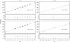 |
Fig. 4 Periods of Table 4 plotted in the Δk – period planes. Filled circles denote average periods by the 9 μHz spacings. The panels on the left and right show the ℓ = 1 and 2 solutions and their linear least-squares fits, respectively. The residuals of the fits are also presented. Top and bottom rows display different solutions by changing some periods’ presumed ℓ values. The resulting period spacings (ΔΠℓ = 1,2) are denoted. |
For g-modes with high radial order k (long periods), the separation of consecutive periods (Δk = 1) becomes nearly constant at a value given by the asymptotic theory of non-radial stellar pulsations. Specifically, the asymptotic period spacing (Tassoul et al. 1990) is given by  (1)where
 ![Mathematical equation: \begin{equation} \label{asympeq} \Pi_0= 2 \pi^2 \left[ \int_{r_1}^{r_2} \frac{N}{r} {\rm d}r\right]^{-1}, \end{equation}](/articles/aa/full_html/2014/10/aa23757-14/aa23757-14-eq137.png) (2)N being the Brunt-Väisälä frequency. In principle, one can compare the asymptotic period spacing computed from a grid of models with different masses and effective temperatures with the mean period spacing exhibited by the star, and then infer the value of the stellar mass. This method has been applied in numerous studies of pulsating PG 1159 stars (see, for instance, Córsico et al. 2007a,b, 2008, 2009a, and references therein). For the method to be valid, the periods exhibited by the pulsating star must be associated with high-order g-modes, that is, the star must be within the asymptotic regime of pulsations. In addition, the star needs to be chemically homogeneous for Eq. (1) to be strictly valid. However, the interior of DB white dwarf stars are assumed to be chemically stratified and characterized by strong chemical gradients built up during the progenitor star life. Therefore the direct application of the asymptotic period spacing to infer the effective temperature and stellar mass of KUV 05134+2605 is questionable. A better way to compare our models with the period spacing of the observed pulsation spectrum is to calculate the average of the computed period spacings, using
(2)N being the Brunt-Väisälä frequency. In principle, one can compare the asymptotic period spacing computed from a grid of models with different masses and effective temperatures with the mean period spacing exhibited by the star, and then infer the value of the stellar mass. This method has been applied in numerous studies of pulsating PG 1159 stars (see, for instance, Córsico et al. 2007a,b, 2008, 2009a, and references therein). For the method to be valid, the periods exhibited by the pulsating star must be associated with high-order g-modes, that is, the star must be within the asymptotic regime of pulsations. In addition, the star needs to be chemically homogeneous for Eq. (1) to be strictly valid. However, the interior of DB white dwarf stars are assumed to be chemically stratified and characterized by strong chemical gradients built up during the progenitor star life. Therefore the direct application of the asymptotic period spacing to infer the effective temperature and stellar mass of KUV 05134+2605 is questionable. A better way to compare our models with the period spacing of the observed pulsation spectrum is to calculate the average of the computed period spacings, using  (3)where ΔΠk is the “forward” period spacing defined as ΔΠk = Πk + 1 − Πk, and n is the number of computed periods located in the range of the observed periods. The theoretical period spacing of the models as computed through Eqs. (1) and (3) shares the same general trends (that is, the same dependence on M∗ and Teff), although
  is usually somewhat higher than
  .
.
As a preliminary mode identification, we attempted to determine the ℓ values of the observed frequencies using not only the effect of rotational splitting, but the derived period-spacing values. The period values of the frequencies are given in Table 4.
Assuming that the frequencies with δf ≈ 9 μHz spacings or its double are ℓ = 1, we created an initial set of the (assumed) ℓ = 1 modes: 527.2, 591.4, 615.9, and 649.1 s. These are the averages of the observed triplet and doublet peaks. In this way, we avoided any assumption on the actual m values. The period differences in this case are 64.3 (2 × 32.2), 24.5, and 33.2 s, respectively. We did not use the average of the peaks at 560 s, but investigated the three frequencies separately.
The effective temperature and surface gravity parameters of KUV 05134+2605 are Teff = 24 700 ± 1300 K and log g = 8.21 ± 0.06 (M∗ = 0.73 ± 0.04 M⊙), from model atmosphere fits to a high signal-to-noise optical spectrum of the star (Bergeron et al. 2011). Bergeron et al. (2011) also found that KUV 05134+2605 belongs to the DBA spectral class, which means that it shows not only helium, but hydrogen lines.
Theoretical calculations show that period spacings of ℓ = 1 modes of 0.7 and 0.8 M∗ model stars can vary between ≈ 25 − 40 s, depending on mode trapping (Bradley et al. 1993). It is also known that the mean period spacing decreases with increasing stellar mass. Figure 8 of Bradley et al. (1993) shows that the minima in the period-spacing diagrams of 0.7 and 0.8 M∗ model stars are ≈ 30 and 25 s for the ℓ = 1 modes, respectively. Trapped modes have lower kinetic energies, and minima in period-spacing diagrams correspond to minima in kinetic energies (Bradley & Winget 1991). Assuming that there is a missing overtone in our period list, the period-spacing values are ≈ 30 s, except for one case with the lower value of 25 s. These are acceptable values of period spacings for this relatively high-mass variable.
Fu et al. (2013) demonstrated for the ZZ Ceti star HS 0507+0434B that the mean period-spacing value can also be determined by the linear least-squares fit of the m = 0 modes plotted in the Δk – period plane. Assuming that most of the observed frequencies correspond to ℓ = 1 modes, we fitted almost all of the periods on the top left panel of Fig. 4, excluding only the periods at 664 and 546 s; because of the high frequency-density in these regions, it seems improbable that they are all ℓ = 1. This solution reflects the expectation that the period differences should be higher and lower than 25 s for the ℓ = 1 and 2 modes, respectively. The formula used for the fits is Pk = P0 + ΔP × Δk (Fu et al. 2013). For the assumed ℓ = 1 modes, we selected the 615.9 s mode as k0.
The top panels of Fig. 4 show the corresponding ℓ = 1 and 2 fits and their residuals. Filled circles denote the four average periods of the assumed ℓ = 1 modes by the 9 μHz spacings. The average ℓ = 1 period spacing determined this way is ΔΠl = 1 = 31.2 ± 0.4 s. We present a possible fit to the two ℓ = 2 periods (ΔΠl = 2 = 16.9 s) for comparison with the next fit’s result.
Because there are some outliers in the ℓ = 1 fit, we assumed that their previously attributed ℓ values are not correct, and in the next step, we moved them to the ℓ = 2 group in an attempt to optimize our fit. The bottom panels of Fig. 4 show the results of this solution. The corresponding ΔΠ values for the ℓ = 1 and 2 modes are 31.4 ± 0.3 and 18.0 ± 0.3 s. The results show that with the change of the ℓ values of some periods, the average period spacings change little. This method alone cannot be used for mode identification, but strongly suggests that even if there are frequencies in our list that are not correctly determined because of the alias ambiguities, the frequencies are not randomly distributed, and especially for the presumed ℓ = 1 modes, this points to a definite mean spacing value.
According to theoretical calculations (e.g. Reed et al. 2011), the asymptotic ratio of the period spacings of ℓ = 1 and 2 modes is  . For the second fits presented above, this ratio is (31.4 ± 0.3) / (18.0 ± 0.3) = 1.74 ± 0.03. That is, the result agrees with the theoretical prediction within the uncertainty.
For the frequency pairs, we can conclude that (1) the 719 and 706 s periods, if both are real pulsation frequencies and not aliases, cannot have the same ℓ, and the 706 s one may be the ℓ = 2. (2) The 686 − 679 s peaks either can be rotationally split or 1 d-1 alias ℓ = 1 or 2 frequencies. (3) According to the period fits, the 561 and 556 s periods may be rotationally split ℓ = 1 frequencies (m = − 1, + 1) and not ℓ = 2 ones. In this case, the 567 s period is an ℓ = 2, and its 18.8 μHz frequency separation with the 561 s peak is a coincidence and has nothing to do with the assumed 9 μHz rotational splitting. (4) The 399 s member of the 395 − 399 s pair fits better into the series of ℓ = 1 modes. The last two columns of Table 4 show the presumed ℓ and m values determined by the assumed rotational multiplets and the period-spacing investigations.
3.4.3. Tests on period spacings
All of our efforts aim to know more about the stellar structure, especially about the mass of the observed object. As we mentioned above, the mean period spacing is an indicator of the stellar mass, and by applying linear fits to the observed periods, we determined 31.4 s for the presumed ℓ = 1 modes. Because of the 1 d-1 alias ambiguities, the reliability of this value must be investigated. We performed several tests to verify our solution.
We searched for a characteristic period spacing between the periods listed in Table 4 by using Kolmogorov-Smirnov (K-S; Kawaler 1988) and inverse variance (I-V; O’Donoghue 1994) significance tests. In the K-S test, the quantity Q is defined as the probability that the observed periods are randomly distributed. Thus, any characteristic period spacings in the period spectrum should appear as a minimum in Q. In the I-V test, a maximum of the I-V will indicate a constant period spacing. Taking all the periods of Table 4, or in other words, without any assumptions based on frequency or period spacings, both methods strongly indicate a characteristic period spacing of about 31 s (see Fig. 5). The minimum in the K-S test is at 31.0 s, while the maximum in the I-V plot is at 31.4 s. These values agree very well with the mean period spacings found by linear fits for ℓ = 1 modes.
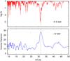 |
Fig. 5 Characteristic spacings of the periods listed in Table 4 as a result from applying Kolmogorov-Smirnov (K-S) and inverse variance (I-V) significance tests. The vertical dotted line denotes the 31.4 s spacing value obtained in Sect. 3.4.2. |
Another well-known method to find a characteristic spacing value is the Fourier analysis of the periods themselves (see e.g. Handler et al. 1997). At first, we performed the Fourier analysis of the periods listed in Table 4 and found a clear maximum at 31.4 s. This also supports the spacing derived by the linear fits and by the K-S and I-V tests. In the next step, we modified the period list: we randomly chose eight frequencies and (also randomly) added or subtracted 11.574 μHz (1 d-1) to these values. That is, we changed almost 40 percent of the periods. Afterwards, we generated a new period list with these modified frequencies, simulating the effect of the 1 d-1 aliasing that is present in all datasets. We generated 20 such aliased period lists and performed Fourier analyses. Applying this Monte Carlo test, we still find a common maximum around 31 s in each simulation. The average of the maxima for the 20 different cases is 31.4 ± 0.2 s.
Finally, we created a period list containing the periods presented in Handler et al. (2003) and marked in Table 4, which were selected as the dominant and well-separated peaks from the different epochs’ datasets. We complemented this with five periods from the Konkoly2007 dataset (686.6, 615.9, 594.6, 439.1, and 395.1 s), and also performed a Fourier analysis. This list only contains 14 periods, but we still obtain a maximum at 31.3 s in the ΔΠ = 25 − 40 s region. Figure 6 shows the FT of the original period set of Table 4, five of the FTs of the aliased period lists, and the FT of the 14-period list.
These tests demonstrate that even if the dataset suffers from alias problems, the results from different methods remain consistent and thus the mean period spacing at 31 s is a robust finding. Considering all of the mean period spacings derived by the linear fits, the K-S, I-V, and Monte Carlo (Fourier) tests, we consider 31.4 ± 0.3 s as the best estimate for the mean spacing of ℓ = 1 modes.
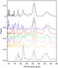 |
Fig. 6 Fourier transforms of different period sets. From top to bottom: FT of the periods of Table 4 (black solid line), test FTs of 5 of the 20 “aliased” period lists (coloured lines), FT of the combined list (black dashed line) using the periods determined by Handler et al. (2003) and five additional periods from the Konkoly2007 dataset (altogether 14 items). The vertical dotted line denotes the 31.4 s spacing value. |
4. Stellar models
4.1. New spectroscopic mass of KUV 05134+2605
We employed the DB white dwarf evolutionary tracks of Córsico et al. (2012) to infer the stellar mass of KUV 05134+2605 from the spectroscopic determination of Teff = 24 700 ± 1300 K and log g = 8.21 ± 0.06 by Bergeron et al. (2011). These tracks cover a wide range of effective temperatures (35 000 ≳ Teff ≳ 18 000 K) and masses (0.51 ≲ M∗/M⊙ ≲ 0.870). The sequences of DB white dwarf models have been obtained with a complete treatment of the evolutionary history of progenitors stars (see Althaus et al. 2009 for details; or Córsico et al. 2012 for a brief discussion). We varied the stellar mass and the effective temperature parameters in our model calculations, while the helium content, the chemical structure at the core, and the thickness of the chemical transition regions were fixed by the evolutionary history of progenitor objects.
In Fig. 7 we plot the evolutionary tracks along with the location of all the DBV stars known to date. We infer a new value of the spectroscopic mass for this star on the basis of this set of evolutionary models. This is relevant because this same set of DB white dwarf models is used in the next sections to derive the stellar mass from the period spacing and the individual pulsation periods of KUV 05134+2605. We found M∗ = 0.72 ± 0.04 M⊙, in agreement with the value quoted in Sect. 3.4.2 (M∗ = 0.73 ± 0.04 M⊙).
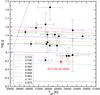 |
Fig. 7 Location of the known DBV stars on the Teff − log g plane. Our DB white dwarf evolutionary tracks are also included and are displayed with different colours according to the stellar mass. The location of KUV 05134+2605 as given by spectroscopy is highlighted with a red asterisk. The theoretical blue edge of the DBV instability strip corresponding to the version MLT2 (α = 1.25) of the MLT theory of convection, as derived by Córsico et al. (2009b), is depicted with a blue dashed line. |
4.2. Clues of the stellar mass from the period spacing
The observed mean period spacing of the dipole modes of KUV 05134+2605, as derived and checked in Sect. 3.4.3, is ΔΠℓ = 1 = 31.4 ± 0.3 s. This period spacing is certainly shorter than the values measured in other DBV stars, that is, EC20058-5234 (ΔΠ = 36.5 s; Bischoff-Kim & Østensen 2011), GD 358 (ΔΠ = 38.8 s; Provencal et al. 2009), and white dwarf J1929+4447 (ΔΠ = 35.9 s; Bischoff-Kim & Østensen 2011). This suggests that KUV 05134+2605 might be more massive than other pulsating stars within the V777 Her class.
In Fig. 8, we show the run of the average of the computed period spacings (Eq. (3)) with ℓ = 1, in terms of the effective temperature for all of our DB white-dwarf evolutionary sequences. The g-mode pulsation periods were computed with the LP-PUL adiabatic pulsation code described in Córsico & Althaus (2006). The curves displayed in the plot are somewhat jagged. This is because the average of the computed period spacings is evaluated for a fixed period interval, and not for a fixed k-interval. As the star evolves towards lower effective temperatures, the periods generally increase with time. At a given Teff, there are n computed periods in the chosen period interval. Later, when the model has cooled enough, it is possible that the accumulated period drift nearly matches the period separation between adjacent modes (| Δk | = 1). In these circumstances, the number of periods in the chosen (fixed) period interval is n ± 1, and exhibits a small jump. To smooth the curves of , we considered pulsation periods in a wider range of periods (100 ≲ Πk ≲ 1200 s) for Fig. 8 than that observed in KUV 05134+2605 (390 ≲ Πk ≲ 780 s)3. The location of KUV 05134+2605 is indicated by a red asterisk according to the solution for ΔΠℓ = 1 (Sect. 3.4.3).
We can estimate the stellar mass free from any possible uncertainty in the spectroscopic analysis. If the possible range of masses for the star is within the DBV instability strip (21 500 ≲ Teff ≲ 29 000 K), then 0.74 ≲ M∗/M⊙ ≲ 1.00. This conclusion relies only on the measured mean period spacing and on the average of the computed period spacing, a global quantity that is not affected by the precise shape of the chemical transition regions of the models. This result is independent of the mass of the He-rich envelope. Indeed, Tassoul et al. (1990) have shown that the asymptotic period spacing of DBV white dwarfs is particularly insensitive to the mass of the He-rich mantle, changing by less than 1 s for a change of ten orders of magnitude in the mass of the He-rich mantle (see their Fig. 42). This conclusion is also independent of the effective temperature of the star. This means that the result that the mass of KUV 05134+2605 is higher than the average mass of DB white dwarfs (see Kepler et al. 2007; Bergeron et al. 2011; Kleinman et al. 2013) is reliable.
If we adopt the spectroscopic effective temperature of KUV 05134+2605 (Teff = 24 700 ± 1300 K) as a constraint, we infer a mass for the star of M∗ = 0.85 ± 0.05 M⊙. This value is higher than the spectroscopic mass (~ 0.72 − 0.73 M⊙). The two estimates of the stellar mass of KUV 05134+2605 are based on the same DB white dwarf evolutionary models, which is a necessary condition for the comparison between the two values to be consistent.
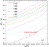 |
Fig. 8 Average of the computed period spacings for ℓ = 1 corresponding to our DB white dwarf sequences with different stellar masses. The location of KUV 05134+2605 is shown with a red asterisk (Teff = 24 700 ± 1300 K) for the observed ΔΠℓ = 1 = 31.4 ± 0.3 solution of mean period spacing. By simple linear interpolation, we found that the mass of the star according to its period spacing is M∗ = 0.85 ± 0.05 M⊙. |
4.3. Constraints from the individual observed periods
The usual way to infer the stellar mass, the effective temperature, and details of the internal structure of pulsating white dwarfs is to investigate their individual pulsation periods. In this approach, we seek a DB white dwarf pulsation model that best matches the pulsation periods of KUV 05134+2605. The goodness of the match between the theoretical pulsation periods (Πk) and the observed individual periods (Πobs,i) is measured by means of a quality function defined as ![Mathematical equation: \begin{equation} \chi^2(M_*, T_{\rm eff})= \frac{1}{N} \sum_{i=1}^{N} \min[(\Pi_{{\rm obs},i}- \Pi_k)^2], \label{ptpf} \end{equation}](/articles/aa/full_html/2014/10/aa23757-14/aa23757-14-eq202.png) (4)where N is the number of observed periods. The DB white dwarf model that shows the lowest value of χ2 is adopted as the best-fit model. Our asteroseismological approach combines (i) a significant exploration of the parameter space; and (ii) detailed and updated input physics, in particular, regarding the internal structure, which is a crucial aspect for correctly separating the information encoded in the pulsation patterns of variable white dwarfs (see Córsico et al. 2007a,b, 2008, 2009a, 2012; Romero et al. 2012, 2013).
(4)where N is the number of observed periods. The DB white dwarf model that shows the lowest value of χ2 is adopted as the best-fit model. Our asteroseismological approach combines (i) a significant exploration of the parameter space; and (ii) detailed and updated input physics, in particular, regarding the internal structure, which is a crucial aspect for correctly separating the information encoded in the pulsation patterns of variable white dwarfs (see Córsico et al. 2007a,b, 2008, 2009a, 2012; Romero et al. 2012, 2013).
We evaluated the function χ2(M∗,Teff) for stellar masses of 0.515,0.530,0.542,0.565,0.584,0.609,0.664,0.741, and 0.870 M⊙. For the effective temperature, we employed a finer grid (ΔTeff = 10 − 30 K). The quality of our period fits was assessed by means of the average of the absolute period differences,  , where δi = Πobs,i − Πk, and by the root-mean-square residual,
 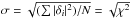 .
.
Because of the unusually many (for DBV standards) pulsation periods observed in KUV 05134+2605, we considered several cases for the set of periods to be employed in our asteroseismological fits.
4.3.1. Case 0
Here, we considered that all the identified periods shown in Table 4 are associated with either ℓ = 1or ℓ = 2, that is, no mixture of ℓ. Because of the small separations between some periods in the pulsation spectrum of KUV 05134+2605, the modes should all be ℓ = 2. However, it is improbable that a pulsating white dwarf shows only quadrupole modes (Winget et al. 1994; Costa et al. 2008), and we discarded this.
4.3.2. Case 1
In this case, we assumed that the periods exhibited by KUV 05134+2605 correspond to a mix of dipole and quadrupole modes. Here, we performed a period fit in which the value of ℓ for the theoretical periods is not fixed at the outset but instead is obtained as an output of our period fit procedure, with the allowed values of ℓ = 1 and ℓ = 2. We assumed as real five rotational multiplets of frequencies and selected the period of the m = 0 component (if present) to perform our period fit. The period corresponding to the average of the frequencies assumed to be the m = − 1 and m = + 1 components if the m = 0 component is absent. We also assumed that the component m = 0 in the assumed triplet at periods in the interval 525.8 − 528.5 s is the period at 525.8 s4. Specifically, we adopted a set of 16 periods.
We investigated the quantity (χ2)-1 in terms of the effective temperature for different stellar masses and found one strong maximum for a model with M∗ = 0.87 M⊙ and Teff = 25 980 K. This pronounced maximum in the inverse of χ2 implies that the theoretical and observed periods agree well. The effective temperature of this model is somewhat higher than (but still agrees with) the spectroscopic effective temperature of KUV 05134+2605 (Teff = 24 700 ± 1300 K). Another maximum, albeit much less pronounced, is encountered for a model with the same stellar mass and lower effective temperature (Teff ~ 24 000 K). However, because the observed and theoretical periods for these models match less well, we adopted the model with Teff = 25 980 K as the best-fit asteroseismological model. To have an indicator of the quality of the period fit, we computed the Bayes information criterion (BIC; Koen & Laney 2000):  (5)where Np is the number of free parameters and N is the number of observed periods. The lower the value of BIC, the better the quality of the fit. In our case, Np = 2 (stellar mass and effective temperature), N = 16, and σ = 2.8 s. We obtained BIC = 1.06, which means that our fit is relatively good.
An important caveat should be kept in mind: from the period-fit procedure, most of the periods are associated with ℓ = 2 modes. This contradicts the well-known property that ℓ = 1 modes exhibit substantially larger amplitudes than ℓ = 2 modes because geometric cancellation effects become increasingly severe as ℓ increases (Dziembowski 1977). As a result of this, pulsating white dwarfs are expected to exhibit preferentially dipole modes. Finally, we note a shortcoming of our asteroseismological model: the pair of close periods at (395.1, 399.2) s is fitted by a single period at 398.1 s.
4.3.3. Case 2
Here, we assumed that the periods close to each other (the period pairs) that cannot be considered as components of triplets with a frequency separation of ~ 9 μHz are a single period. We considered the period resulting from the average of the frequencies present. That is, we replaced the pair (395.1, 399.2) s by a single period at 397.2 s, the pair (679.1, 686.6) s by a period at 682.8 s, and the pair (706.8, 719.1) s by a period at 712.9 s. The reduced list contains 13 periods. In this case, the best-fit model has M∗ = 0.87 M⊙ and Teff = 25 890 K [ (χ2)-1 ~ 0.13 ], thus the solution found in Case 1 still persists. However, in this case, other solutions [Teff ~ 27 100 K, (χ2)-1 ~ 0.12, and Teff ~ 24 150 K, (χ2)-1 ~ 0.11] with the same stellar mass are equally valid from a statistical point of view. The number of ℓ = 2 modes still exceeds the number of ℓ = 1 modes in the fit.
4.3.4. Case 3
At variance with the previous cases, here we assumed the ℓ-identification shown in Table 4 to be correct and then constrained the ℓ = 1 observed modes to be fitted by ℓ = 1 theoretical modes, and the ℓ = 2 observed modes to be fitted by ℓ = 2 theoretical modes. According to Table 4, there are several possible assumptions for the mode identification. Specifically, the period at 439.1 s can be associated with ℓ = 1 or ℓ = 2; the m = 0 component in the (525.8, 528.5) s doublet can be either 525.8 s or 528.5 s; and the period at 679.1 s may be associated with ℓ = 1 and the period at 686.6 s to ℓ = 2, or vice versa. On the other hand, the period at 395.1 s must be an ℓ = 2 mode if the period at 399.2 s is an ℓ = 1 mode. Similarly, the 706.8 s period must be associated with ℓ = 2 if the 719.1 s period is an ℓ = 1 mode. We have taken into account all the possible combinations in our period fits. Regardless of the assumptions we adopted for the periods at 439.1 s, 525.8 s, 528.5 s, 679.1 s, and 686.6 s, we obtained a clear and recurrent single solution for a model with M∗ = 0.87 M⊙ and Teff = 24 060 K. The set of observed periods and their assigned ℓ values (9 modes with ℓ = 1 and 7 modes with ℓ = 2) are listed in the first two columns of Table 5. The theoretical periods of this fit are shown in the third column of this table, and the results of the period fit are displayed in Fig. 9. The quality of the fit is described by a BIC index of 1.17.
Comparison between the observed 16 periods and theoretical (ℓ = 1,2) periods corresponding to the seismological solutions in Case 3 (Cols. 3 and 4), with M∗ = 0.87 M⊙ and Teff = 24 060 K, and considering the additional evolutionary sequences with masses between M∗ = 0.74 M⊙ and M∗ = 0.87 M⊙ (Cols. 5 and 6, Πk,zoom and kzoom).
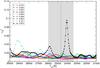 |
Fig. 9 Inverse of the quality function of the period fit in terms of the effective temperature for Case 3. The vertical grey strip indicates the spectroscopic Teff and its uncertainties (Teff = 24 700 ± 1300 K). |
4.4. Zooming-in on the best-fit model region
To search for possible closer solutions in the region of the parameter space where the best-fit model from period-to-period fits (M∗ ~ 0.87 M⊙) was found, we extended our exploration by generating a set of additional DB white dwarf evolutionary sequences with masses between 0.74 M⊙ and 0.87 M⊙. These sequences were constructed by scaling the stellar mass from the 0.87 M⊙ sequence at very high effective temperatures. The internal chemical profiles (of utmost importance for the pulsation properties of white dwarfs) of these new sequences are consistently assessed through linear interpolation between the chemical profiles of the sequences with 0.74 M⊙ and 0.87 M⊙.
Specifically, we computed ℓ = 1,2g-mode periods of these additional sequences with M∗ = 0.76, 0.78, 0.80, 0.805, 0.82, 0.84, 0.85, 0.86 M⊙, and carried out period fits to these models. We discuss Case 3 in detail. The main results of the period fits are displayed in Fig. 10. The best solution is a model with a stellar mass of 0.84 M⊙ and an effective temperature of 25 050 K, characterized by a BIC index of 1.06, which is slightly lower than for Case 3.
This period fit corresponds to the case in which the period at 439.1 s is associated with ℓ = 1, the m = 0 component in the (525.8, 528.5) s doublet is assumed to be at 525.8 s, the period at 679.1 s is an ℓ = 1, and the period at 686.6 s is an ℓ = 2 mode. We also searched for asteroseismological solutions taking other combinations of these assumptions into account. Interestingly, the assignation of the harmonic degree to the periods at 679.1 s and 686.6 s proved to be crucial for our results. Specifically, we obtained the solution (M∗/M⊙,Teff) = (0.84,25 050 K) whenever we assumed that the period at 679.1 s is an ℓ = 1, and the 686.6 s period is an ℓ = 2 mode. If not, we obtained a second seismological solution with M∗ = 0.82 M⊙ and Teff = 25 700 K. The quality of the period fit, however, is poorer (BIC = 1.19). We also performed fits replacing the pair (679.1, 686.6) s by a single period at 682.8 s. Assuming that this (average) period is ℓ = 1, the best-fit solution is M∗ = 0.85 M⊙ and Teff = 24 690 K. The preferred model is M∗ = 0.84 M⊙ and Teff = 25 050 K, if the 682.8 s period is ℓ = 2. Finally, we adopted the model with (M∗/M⊙,Teff) = (0.84,25 050 K), when the 679.1 s period is an ℓ = 1 and the 686.6 s period is an ℓ = 2, as our asteroseismological solution for KUV 05134+2605. This solution is characterized by the lowest BIC index and has an effective temperature that agrees excellently with the value predicted by spectroscopy. The set of theoretical periods of this fit is listed in Table 5 (Col. 5).
4.4.1. Best-fit model
The main features of our best-fit model considering the additional evolutionary sequences are summarized in Table 6, where we also include the parameters from spectroscopy (Bergeron et al. 2011). In the table, the quantity MHe corresponds to the total content of He of the envelope of the model.
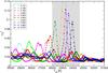 |
Fig. 10 Same as in Fig. 9, but restricted to the set of model sequences with masses between 0.74 M⊙ and 0.87 M⊙. |
We briefly describe the main properties of our best-fit DB model for KUV 05134+2605. In Fig. 11, we depict the internal chemical structure of this model (upper panel), where the abundance by mass of the main constituents (4He, 12C, and 16O) is shown in terms of the outer mass fraction [− log (1 − Mr/M∗)]. The chemical structure of our models consists of a C/O core − resulting from the core He burning of the previous evolution − shaped by processes of additional mixing, for example, overshooting. The core is surrounded by a mantle rich in He, C, and O, which is the remnant of the regions altered by the nucleosynthesis during the thermally pulsing asymptotic giant branch. Above this shell, there is a pure He mantle with a mass MHe/M∗ ~ 1.4 × 10⁻³, constructed by the action of gravitational settling that causes He to float to the surface and heavier species to sink.
The lower panel of Fig. 11 displays the run of the two critical frequencies of non-radial stellar pulsations, that is, the Brunt-Väisälä frequency and the Lamb frequency (Lℓ) for ℓ = 1. The precise shape of the Brunt-Väisälä frequency largely determines the properties of the g-mode period spectrum of the model. In particular, each chemical gradient in the model contributes locally to the value of N. The most notable feature is the highly peaked structure at the C/O chemical transition [− log (1 − Mr/M∗) ~ 0.5]. On the other hand, the He/C/O transition region at − log (1 − Mr/M∗) ~ 2 − 5 is very smooth and does not affect the pulsation spectrum much.
Main characteristics of KUV 05134+2605 and our best-fit model considering the additional evolutionary sequences with masses between M∗ = 0.74 M⊙ and M∗ = 0.87 M⊙.
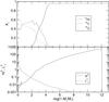 |
Fig. 11 Internal chemical structure (upper panel) and the squared Brunt-Vaïsälä and Lamb frequencies for ℓ = 1 (lower panel) corresponding to our best-fit DB white dwarf model with a stellar mass M∗ = 0.84 M⊙, an effective temperature Teff = 25 050 K, and a He envelope mass of MHe/M∗ ~ 1.5 × 10⁻³. |
4.4.2. Periods from a DBA model
Bergeron et al. (2011) reported that KUV 05134+2605 belongs to the DBA spectral class. Therefore, we performed exploratory computations of the period spectrum of a DB white dwarf model with pure helium atmosphere (“DB model”) and a similar model that has small impurities of hydrogen (“DBA model”). In the DBA model, the hydrogen is mixed with helium throughout the helium envelope (as in the DBA models of Córsico et al. 2009b, Sect. 4). Both models have M∗ = 0.74 M⊙ and Teff ~ 24 600 K. In particular, we analysed the case in which log (NH/NHe) ~ − 3.8 (the value corresponding to KUV 05134+2605 according to Bergeron et al. 2011).
We found that the relative differences in the pulsation periods of these two models are on average lower than 0.2%. This means an absolute difference lower than 0.8 s for periods around 400 s, and below 1.6 s for periods around 800 s. That is, the presence of small abundances of hydrogen in the almost pure helium atmospheres of DB white dwarfs does not significantly alter the pulsation periods. As a result, pure helium envelope models like those we employed in this study are suitable for asteroseismic modelling of DBA white dwarfs like KUV 05134+2605.
5. Summary and conclusions
The almost continuous, high-precision light curves provided by photometric space missions completely revolutionized the variable star studies in many fields. However, up to now, only one V777 Her and three ZZ Ceti stars were monitored from space (Greiss et al. 2014; Hermes et al. 2011; Østensen et al. 2011; Hermes et al. 2014). This means that exploring their pulsational properties and thus studying their interiors is still mainly based on ground-based observations. Even though their pulsation periods are short, in many cases extended observations (e.g. multi-site campaigns and/or at least one season-long monitoring) are needed to determine enough (at least half a dozen) normal modes for asteroseismic investigations (see e.g. the cases of KUV 02464+3239, Bognár et al. 2009, and GD 154, Paparó et al. 2013). Otherwise, the few detected modes can result in models with fairly different physical parameters that can fit the observed periods similarly well. This shows the particular importance of the rich pulsators, in which at least a dozen normal modes can be fitted. Amplitude variations on short time-scales seem to be common among the white dwarf pulsators. This can help to detect new modes because from observing the star in different epochs we can find new frequencies and complement the list of known excited modes.
For KUV 05134+2605, we used photometric datasets obtained in seven different epochs between 1988 and 2011. We re-analysed the data published by Handler et al. (2003) and also collected data at the Piszkéstető mountain station of Konkoly Observatory in two different observing seasons. Comparing the frequency content of the different datasets and considering the results of the frequency determination tests, we arrived at 22 pulsation frequencies between 1280 and 2530 μHz. The frequency grouping suggests at least 12 possible modes for the asteroseismic model fits. With this, KUV 05134+2605 joined the – not populous – group of rich white dwarf pulsators. We also showed that considering a ≈ 9 μHz frequency separation, one triplet and at least one doublet can be determined. Assuming that the frequencies showing the ≈ 9 μHz separation are ℓ = 1 modes, we estimated the stellar rotation period to be 0.6 d. We determined a 31 s mean period spacing using different methods, such as linear fits to the observed periods, Kolmogorov-Smirnov and inverse variance tests, and Fourier analyses of different period lists. We also simulated the effect of alias ambiguities on the mean period-spacing determination. All of the results were consistent and point to the 31 s characteristic spacing for the dipole modes.
The extended list of frequencies provided the opportunity for asteroseismic investigations of KUV 05134+2605 for the first time. For period-to-period fits, the effective temperature of the selected model is Teff = 25 050 K, which is the same as the spectroscopic temperature (Teff = 24 700 ± 1300 K, Bergeron et al. 2011) within the uncertainties. This model’s helium layer mass is 1.2 × 10⁻³M⊙.
The stellar mass derived from the period spacing data and the period-to-period fits agreed excellently well, all providing M∗ = 0.84 − 0.85 M⊙ solutions. The mass inferred from spectroscopy is 17 − 18% lower than these values. One should keep in mind, however, that around the V777 Her instability strip, the helium lines are at maximum strength and therefore there is an ambiguity about a hot and a cool solution, just like the ambiguity of the high and low mass from the asteroseismological side. There also remain uncertainties in the synthetic line profile calculations. Similarly, we made assumptions on the physics of stars in the asteroseismic modelling. It is beyond the scope of this paper to discuss which method is better suited to estimate the stellar mass and why.
Therefore, we consider the agreement between the results of three methods to be satisfactory. All three methods result in a mass for KUV 05134+2605 higher than the average mass of DB white dwarfs. Moreover, our study suggests that this star is the most massive of the known DBVs.
IRAF is distributed by the National Optical Astronomy Observatories, which are operated by the Association of Universities for Research in Astronomy, Inc., under cooperative agreement with the National Science Foundation.
If we adopt a shorter range of periods, closer to the range of periods exhibited by KUV 05134+2605 (e.g. 390−780 s), the curves we obtain are much more irregular and jagged, although the results do not change much.
We also considered the case in which the period adopted is 528.5 s and the situation in which the pair (525.8, 528.5) s is not really a multiplet, but instead two distinct modes with different ℓ-values. We obtained results almost identical to those described in this section, similar to Metcalfe (2003).
Acknowledgments
The authors thank the anonymous referee for the constructive comments and recommendations on the manuscript. We thank Gerald Handler for providing the KUV 05134+2605 data obtained in 1988, 1992, 2000 October, 2001, and during the Whole Earth Telescope campaign in 2000 (XCov20). The authors also acknowledge the contribution of L. Molnár, E. Plachy, H. Ollé and E. Verebélyi to the observations of KUV 05134+2605. We thank Ádám Sódor for critically reading the manuscript and his useful comments. Zs.B. acknowledges the support of the Hungarian Eötvös Fellowship (2013) and the kind hospitality of the Royal Observatory of Belgium as a temporary voluntary researcher (2013–2014). Zs.B. and M.P. acknowledge the support of the ESA PECS project 4000103541/11/NL/KML.
References
- Althaus, L. G.. Panei, J. A.. Miller Bertolami, M. M., et al. 2009, ApJ, 704, 1605 [NASA ADS] [CrossRef] [Google Scholar]
- Althaus, L. G., Córsico, A. H., Isern, J., & García-Berro, E. 2010, A&ARv, 18, 471 [NASA ADS] [CrossRef] [Google Scholar]
- Bergeron, P., Wesemael, F., Dufour, P., et al. 2011, ApJ, 737, 28 [NASA ADS] [CrossRef] [EDP Sciences] [Google Scholar]
- Bischoff-Kim, A. 2009, in AIP Conf. Ser., 1170, eds. J. A. Guzik, & P. A. Bradley, 621 [Google Scholar]
- Bischoff-Kim, A., & Metcalfe, T. S. 2012, in Progress in Solar/Stellar Physics with Helio- and Asteroseismology, eds. H. Shibahashi, M. Takata, & A. E. Lynas-Gray, ASP Conf. Ser., 462, 164 [Google Scholar]
- Bischoff-Kim, A., & Østensen, R. H. 2011, ApJ, 742, L16 [NASA ADS] [CrossRef] [Google Scholar]
- Bognár, Zs., Paparó, M., Bradley, P. A., & Bischoff-Kim, A. 2009, MNRAS, 399, 1954 [NASA ADS] [CrossRef] [Google Scholar]
- Bradley, P. A., & Winget, D. E. 1991, ApJS, 75, 463 [NASA ADS] [CrossRef] [Google Scholar]
- Bradley, P. A., Winget, D. E., & Wood, M. A. 1993, ApJ, 406, 661 [NASA ADS] [CrossRef] [Google Scholar]
- Castanheira, B. G., & Kepler, S. O. 2008, MNRAS, 385, 430 [Google Scholar]
- Córsico, A. H., & Althaus, L. G. 2006, A&A, 454, 863 [NASA ADS] [CrossRef] [EDP Sciences] [Google Scholar]
- Córsico, A. H.. Althaus, L. G.. Miller Bertolami, M. M., & Werner, K. 2007a, A&A, 461, 1095 [NASA ADS] [CrossRef] [EDP Sciences] [Google Scholar]
- Córsico, A. H.. Miller Bertolami, M. M., Althaus, L. G., Vauclair, G., & Werner, K. 2007b, A&A, 475, 619 [NASA ADS] [CrossRef] [EDP Sciences] [Google Scholar]
- Córsico, A. H.. Althaus, L. G.. Kepler, S. O.. Costa, J. E. S.. & Miller Bertolami, M. M. 2008, A&A, 478, 869 [NASA ADS] [CrossRef] [EDP Sciences] [Google Scholar]
- Córsico, A. H.. Althaus, L. G.. Miller Bertolami, M. M., & García-Berro, E. 2009a, A&A, 499, 257 [NASA ADS] [CrossRef] [EDP Sciences] [Google Scholar]
- Córsico, A. H.. Althaus, L. G.. Miller Bertolami, M. M., & García-Berro, E. 2009b, J. Phys. Conf. Ser., 172, 012075 [NASA ADS] [CrossRef] [Google Scholar]
- Córsico, A. H.. Althaus, L. G.. Miller Bertolami, M. M., & Bischoff-Kim, A. 2012, A&A, 541, A42 [NASA ADS] [CrossRef] [EDP Sciences] [Google Scholar]
- Costa, J. E. S., Kepler, S. O., Winget, D. E., et al. 2008, A&A, 477, 627 [NASA ADS] [CrossRef] [EDP Sciences] [Google Scholar]
- Csubry, Z., & Kolláth, Z. 2004, in SOHO 14 Helio- and Asteroseismology: Towards a Golden Future, ed. D. Danesy, ESA SP, 559, 396 [Google Scholar]
- Dziembowski, W. 1977, Acta Astron., 27, 1 [NASA ADS] [Google Scholar]
- Eastman, J., Siverd, R., & Gaudi, B. S. 2010, PASP, 122, 935 [NASA ADS] [CrossRef] [Google Scholar]
- Fontaine, G., & Brassard, P. 2008, PASP, 120, 1043 [NASA ADS] [CrossRef] [Google Scholar]
- Fu, J.-N., Dolez, N., Vauclair, G., et al. 2013, MNRAS, 429, 1585 [NASA ADS] [CrossRef] [Google Scholar]
- Grauer, A. D., Wegner, G., Green, R. F., & Liebert, J. 1989, AJ, 98, 2221 [NASA ADS] [CrossRef] [Google Scholar]
- Greiss, S., Gänsicke, B. T., Hermes, J. J., et al. 2014, MNRAS, 438, 3086 [NASA ADS] [CrossRef] [Google Scholar]
- Handler, G.. Pikall, H.. O’Donoghue, D., et al. 1997, MNRAS, 286, 303 [NASA ADS] [CrossRef] [Google Scholar]
- Handler, G., Metcalfe, T. S., & Wood, M. A. 2002, MNRAS, 335, 698 [NASA ADS] [CrossRef] [Google Scholar]
- Handler, G.. O’Donoghue, D., Müller, M., et al. 2003, MNRAS, 340, 1031 [NASA ADS] [CrossRef] [Google Scholar]
- Hermes, J. J., Mullally, F., Østensen, R. H., et al. 2011, ApJ, 741, L16 [NASA ADS] [CrossRef] [Google Scholar]
- Hermes, J. J., Montgomery, M. H., Gianninas, A., et al. 2013, MNRAS, 436, 3573 [NASA ADS] [CrossRef] [Google Scholar]
- Hermes, J. J., Charpinet, S., Barclay, T., et al. 2014, ApJ, 789, 85 [NASA ADS] [CrossRef] [Google Scholar]
- Jones, P. W., Hansen, C. J., Pesnell, W. D., & Kawaler, S. D. 1989, ApJ, 336, 403 [NASA ADS] [CrossRef] [Google Scholar]
- Kawaler, S. D. 1988, in Advances in Helio- and Asteroseismology, eds. J. Christensen-Dalsgaard, & S. Frandsen, IAU Symp., 123, 329 [Google Scholar]
- Kawaler, S. D., Sekii, T., & Gough, D. 1999, ApJ, 516, 349 [NASA ADS] [CrossRef] [Google Scholar]
- Kepler, S. O., Nather, R. E., Winget, D. E., et al. 2003, A&A, 401, 639 [NASA ADS] [CrossRef] [EDP Sciences] [Google Scholar]
- Kepler, S. O., Kleinman, S. J., Nitta, A., et al. 2007, MNRAS, 375, 1315 [NASA ADS] [CrossRef] [Google Scholar]
- Kleinman, S. J., Nather, R. E., Winget, D. E., et al. 1998, ApJ, 495, 424 [NASA ADS] [CrossRef] [Google Scholar]
- Kleinman, S. J., Kepler, S. O., Koester, D., et al. 2013, ApJS, 204, 5 [NASA ADS] [CrossRef] [MathSciNet] [Google Scholar]
- Koen, C., & Laney, D. 2000, MNRAS, 311, 636 [NASA ADS] [CrossRef] [Google Scholar]
- Kolláth, Z. 1990, Konkoly Observatory Occasional Technical Notes, 1, 1 [Google Scholar]
- Lenz, P., & Breger, M. 2005, Comm. Asteroseismol., 146, 53 [Google Scholar]
- Metcalfe, T. S. 2003, Balt. Astron., 12, 247 [NASA ADS] [Google Scholar]
- Montgomery, M. H., Provencal, J. L., Kanaan, A., et al. 2010, ApJ, 716, 84 [NASA ADS] [CrossRef] [Google Scholar]
- Nather, R. E., Winget, D. E., Clemens, J. C., Hansen, C. J., & Hine, B. P. 1990, ApJ, 361, 309 [NASA ADS] [CrossRef] [Google Scholar]
- O’Donoghue, D. 1994, MNRAS, 270, 222 [NASA ADS] [CrossRef] [Google Scholar]
- Østensen, R. H., Bloemen, S., Vučković, M., et al. 2011, ApJ, 736, L39 [NASA ADS] [CrossRef] [Google Scholar]
- Paparó, M., Bognár, Zs., Plachy, E., Molnár, L., & Bradley, P. A. 2013, MNRAS, 432, 598 [NASA ADS] [CrossRef] [Google Scholar]
- Provencal, J. L., Montgomery, M. H., Kanaan, A., et al. 2009, ApJ, 693, 564 [NASA ADS] [CrossRef] [Google Scholar]
- Provencal, J. L., Montgomery, M. H., Kanaan, A., et al. 2012, ApJ, 751, 91 [NASA ADS] [CrossRef] [Google Scholar]
- Reed, M. D., Baran, A., Quint, A. C., et al. 2011, MNRAS, 414, 2885 [Google Scholar]
- Reegen, P. 2007, A&A, 467, 1353 [NASA ADS] [CrossRef] [EDP Sciences] [Google Scholar]
- Romero, A. D., Córsico, A. H., Althaus, L. G., et al. 2012, MNRAS, 420, 1462 [Google Scholar]
- Romero, A. D., Kepler, S. O., Córsico, A. H., Althaus, L. G., & Fraga, L. 2013, ApJ, 779, 58 [NASA ADS] [CrossRef] [Google Scholar]
- Tassoul, M., Fontaine, G., & Winget, D. E. 1990, ApJS, 72, 335 [Google Scholar]
- Van Grootel, V., Fontaine, G., Brassard, P., & Dupret, M.-A. 2013, ApJ, 762, 57 [NASA ADS] [CrossRef] [Google Scholar]
- Vauclair, G., Fu, J.-N., Solheim, J.-E., et al. 2011, A&A, 528, A5 [NASA ADS] [CrossRef] [EDP Sciences] [Google Scholar]
- Winget, D. E., & Kepler, S. O. 2008, ARA&A, 46, 157 [NASA ADS] [CrossRef] [EDP Sciences] [Google Scholar]
- Winget, D. E., Robinson, E. L., Nather, R. D., & Fontaine, G. 1982, ApJ, 262, L11 [NASA ADS] [CrossRef] [Google Scholar]
- Winget, D. E., Nather, R. E., Clemens, J. C., et al. 1991, ApJ, 378, 326 [NASA ADS] [CrossRef] [Google Scholar]
- Winget, D. E., Nather, R. E., Clemens, J. C., et al. 1994, ApJ, 430, 839 [NASA ADS] [CrossRef] [Google Scholar]
- Zima, W. 2008, Commun. Asteroseismo., 155, 17 [NASA ADS] [CrossRef] [Google Scholar]
All Tables
Log of observations of KUV 05134+2605, performed at Piszkéstető, Konkoly Observatory.
Results of the frequency analyses of the datasets from different observing seasons.
Comparison between the observed 16 periods and theoretical (ℓ = 1,2) periods corresponding to the seismological solutions in Case 3 (Cols. 3 and 4), with M∗ = 0.87 M⊙ and Teff = 24 060 K, and considering the additional evolutionary sequences with masses between M∗ = 0.74 M⊙ and M∗ = 0.87 M⊙ (Cols. 5 and 6, Πk,zoom and kzoom).
Main characteristics of KUV 05134+2605 and our best-fit model considering the additional evolutionary sequences with masses between M∗ = 0.74 M⊙ and M∗ = 0.87 M⊙.
All Figures
|
Fig. 1 One of the CCD frames obtained at Piszkéstető, Konkoly Observatory, with the variable and comparison stars marked. The field of view is ≈ 7′ × 7′. |
| In the text | |
|
Fig. 2 Normalized differential light curves of the Konkoly runs. Data were collected in the 2007/2008 observing season (upper panels) and in 2011 (lower panels). For better visibility of the pulsation cycles, we connected the points with grey lines. Boldface numbers in the corners correspond to the run numbers in Table 1. |
| In the text | |
|
Fig. 3 Successive pre-whitening steps of the analyses of the WET2000 and Konkoly2007 datasets. The window functions are given in the insets. Dashed lines denote the 4 ⟨ A ⟩ significance levels calculated by the moving average of the spectra. |
| In the text | |
|
Fig. 4 Periods of Table 4 plotted in the Δk – period planes. Filled circles denote average periods by the 9 μHz spacings. The panels on the left and right show the ℓ = 1 and 2 solutions and their linear least-squares fits, respectively. The residuals of the fits are also presented. Top and bottom rows display different solutions by changing some periods’ presumed ℓ values. The resulting period spacings (ΔΠℓ = 1,2) are denoted. |
| In the text | |
|
Fig. 5 Characteristic spacings of the periods listed in Table 4 as a result from applying Kolmogorov-Smirnov (K-S) and inverse variance (I-V) significance tests. The vertical dotted line denotes the 31.4 s spacing value obtained in Sect. 3.4.2. |
| In the text | |
|
Fig. 6 Fourier transforms of different period sets. From top to bottom: FT of the periods of Table 4 (black solid line), test FTs of 5 of the 20 “aliased” period lists (coloured lines), FT of the combined list (black dashed line) using the periods determined by Handler et al. (2003) and five additional periods from the Konkoly2007 dataset (altogether 14 items). The vertical dotted line denotes the 31.4 s spacing value. |
| In the text | |
|
Fig. 7 Location of the known DBV stars on the Teff − log g plane. Our DB white dwarf evolutionary tracks are also included and are displayed with different colours according to the stellar mass. The location of KUV 05134+2605 as given by spectroscopy is highlighted with a red asterisk. The theoretical blue edge of the DBV instability strip corresponding to the version MLT2 (α = 1.25) of the MLT theory of convection, as derived by Córsico et al. (2009b), is depicted with a blue dashed line. |
| In the text | |
|
Fig. 8 Average of the computed period spacings for ℓ = 1 corresponding to our DB white dwarf sequences with different stellar masses. The location of KUV 05134+2605 is shown with a red asterisk (Teff = 24 700 ± 1300 K) for the observed ΔΠℓ = 1 = 31.4 ± 0.3 solution of mean period spacing. By simple linear interpolation, we found that the mass of the star according to its period spacing is M∗ = 0.85 ± 0.05 M⊙. |
| In the text | |
|
Fig. 9 Inverse of the quality function of the period fit in terms of the effective temperature for Case 3. The vertical grey strip indicates the spectroscopic Teff and its uncertainties (Teff = 24 700 ± 1300 K). |
| In the text | |
|
Fig. 10 Same as in Fig. 9, but restricted to the set of model sequences with masses between 0.74 M⊙ and 0.87 M⊙. |
| In the text | |
|
Fig. 11 Internal chemical structure (upper panel) and the squared Brunt-Vaïsälä and Lamb frequencies for ℓ = 1 (lower panel) corresponding to our best-fit DB white dwarf model with a stellar mass M∗ = 0.84 M⊙, an effective temperature Teff = 25 050 K, and a He envelope mass of MHe/M∗ ~ 1.5 × 10⁻³. |
| In the text | |
Current usage metrics show cumulative count of Article Views (full-text article views including HTML views, PDF and ePub downloads, according to the available data) and Abstracts Views on Vision4Press platform.
Data correspond to usage on the plateform after 2015. The current usage metrics is available 48-96 hours after online publication and is updated daily on week days.
Initial download of the metrics may take a while.