| Issue |
A&A
Volume 570, October 2014
|
|
|---|---|---|
| Article Number | A15 | |
| Number of page(s) | 10 | |
| Section | Interstellar and circumstellar matter | |
| DOI | https://doi.org/10.1051/0004-6361/201423603 | |
| Published online | 07 October 2014 | |
The W43-MM1 mini-starburst ridge, a test for star formation efficiency models⋆
1 Laboratoire AIM Paris-Saclay, CEA/IRFU – CNRS/INSU – Université Paris Diderot, Service d’Astrophysique, Bât. 709, CEA-Saclay, 91191 Gif-sur-Yvette Cedex, France
e-mail: This email address is being protected from spambots. You need JavaScript enabled to view it.
2 Harvard-Smithsonian Center for Astrophysics, Cambridge MA, USA
3 Scottish Universities Physics Alliance (SUPA), School of Physics and Astronomy, University of St. Andrews, North Haugh, St Andrews, Fife KY16 9SS, UK
4 OASU/LAB-UMR 5804, CNRS/INSU – Université Bordeaux 1, 2 rue de l’Observatoire, BP 89, 33270 Floirac, France
5 LERMA, UMR 8112 du CNRS, Observatoire de Paris, École Normale Supérieure, 24 rue Lhomond, 75231 Paris Cedex 05, France
6 Joint ALMA ObservatoryAlonso de Cordova 3107, 763 0355 Vitacura Santiago Chile
7 Institut de Radioastronomie Millimétrique (IRAM), 300 rue de la Piscine, 38406 Saint Martin d’Hères, France
8 School of Physics and Astronomy, Cardiff University, Queens Buildings, The Parade, Cardiff CF24 3AA, UK
9 School of Physics and Astronomy, University of Exeter, Stocker Road, Exeter EX4 4QL, UK
10 Physikalisches Institut, Universität zu Köln, Zülpicher Str. 77, 50937 Köln, Germany
11 LERMA2, Observatoire de Paris, 61 Av. de l’Observatoire, 75014 Paris, France
12 Max-Planck-Institut für Radioastronomie, Auf dem Hügel 69, 53121 Bonn, Germany
13 Canadian Institute for Theoretical Astrophysics, University of Toronto, 60 St. George Street, Toronto, ON M5S 3H8, Canada
14 California Institute of Technology, Pasadena CA 91125, USA
15 Sorbonne Universités, Université Pierre et Marie Curie, Paris 6, CNRS, Observatoire de Paris, UMR 8112, LERMA, Paris, France
Received: 9 February 2014
Accepted: 23 May 2014
Abstract
Context. Star formation efficiency (SFE) theories are currently based on statistical distributions of turbulent cloud structures and a simple model of star formation from cores. They remain poorly tested, especially at the highest densities.
Aims. We investigate the effects of gas density on the SFE through measurements of the core formation efficiency (CFE). With a total mass of ~2 × 10⁴ M⊙, the W43-MM1 ridge is one of the most convincing candidate precursors of Galactic starburst clusters and thus one of the best places to investigate star formation.
Methods. We used high-angular resolution maps obtained at 3 mm and 1 mm within the W43-MM1 ridge with the IRAM Plateau de Bure Interferometer to reveal a cluster of 11 massive dense cores, and, one of the most massive protostellar cores known. A Herschel column density image provided the mass distribution of the cloud gas. We then measured the “instantaneous” CFE and estimated the SFE and the star formation rate (SFR) within subregions of the W43-MM1 ridge.
Results. The high SFE found in the ridge (~6% enclosed in ~8 pc3) confirms its ability to form a starburst cluster. There is, however, a clear lack of dense cores in the eastern part of the ridge, which may be currently assembling. The CFE and the SFE are observed to increase with volume gas density, while the SFR per free fall time steeply decreases with the virial parameter, αvir. Statistical models of the SFR may describe the outskirts of the W43-MM1 ridge well, but struggle to reproduce its inner part, which corresponds to measurements at low αvir. It may be that ridges do not follow the log-normal density distribution, Larson relations, and stationary conditions forced in the statistical SFR models.
Key words: stars: formation / stars: protostars / stars: massive / ISM: clouds / submillimeter: ISM / submillimeter: stars
Final IRAM/PdBI FITS cube is only available at the CDS via anonymous ftp to cdsarc.u-strasbg.fr (130.79.128.5) or via http://cdsarc.u-strasbg.fr/viz-bin/qcat?J/A+A/570/A15
© ESO, 2014
1. Introduction
The formation of high-mass stars remains poorly understood, but an emerging scenario suggests that they form in massive dense cores (MDCs: ~0.1 pc and >105 cm-3 as defined in Motte et al. 2007; see also Wang et al. 2014) through dynamical processes, such as colliding flows initiated by cloud formation (e.g. Csengeri et al. 2011; Nguyen Luong et al. 2013). The Herschel key program HOBYS (see Motte et al. 2010, 2012) identifies ridges as high-density filaments, above 1023 cm-2 in column density, which is favorable to the formation of high-mass (OB-type, ≥8 M⊙) stars (see Hill et al. 2011; Nguyen Luong et al. 2011a; Hennemann et al. 2012). The most extreme of these ridges, W43-MM1, lies in the massive, highly concentrated and very dynamic W43 molecular complex located at 6 kpc (Nguyen Luong et al. 2011b; Carlhoff et al. 2013). In its central region, W43-MM1 is thought to be experiencing a cloud collision (Nguyen Luong et al. 2013), causing a remarkably efficient burst of high-mass star formation (Motte et al. 2003). The W43-MM1 ridge can be modeled by a 3.9 pc × 2 pc × 2 pc ellipsoid with a total mass of ~2 × 10⁴ M⊙ and an average density of ~4.3 ×104 cm-3, which is physically large and massive enough to form a large cluster. Its fragmentation has been studied before with 0.2 pc resolution by Motte et al. (2003). Fragmentation, magnetic field, outflows, and the hot core of the densest part of the W43-MM1 ridge has also been observed with high angular resolution by Cortes & Crutcher (2006) and Sridharan et al. (2014).
Main observational parameters.
A handful of studies have been carried out to estimate the core formation efficiency (CFE) in high-mass star-forming regions, and it has been suggested that the stellar formation efficiency (SFE) increases with gas density (Bontemps et al. 2010; Palau et al. 2013). As for the stellar formation rates (SFRs), most statistical models directly relate it to the amount of gas above a given density threshold (Krumholz & McKee 2005; Padoan & Nordlund 2011; Hennebelle & Chabrier 2011). If this view agrees with the SFR measurements in low-mass star-forming clouds (Heiderman et al. 2010), which are found to be proportional to cloud masses (Eq. (3) of Lada et al. 2010; Evans et al. 2014), they are not representative of typical Galactic clouds forming high-mass stars (Motte et al. 2003; Nguyen Luong et al. 2011a). These observational differences cast doubt on the accuracy of extrapolating scaling laws observed in low-mass star-forming regions to describe star formation in clouds forming high-mass stars.
MDCs hosting high-mass protostars can be used to investigate the fragmentation of ridges and measure the concentration of its gas into high-density seeds and then high-mass stars.
In the present paper1, we investigate the CFE variations through the W43-MM1 ridge and compare the resulting SFE and SFR estimates to predictions of star formation models. Section 2 presents an interferometric imaging of W43-MM1 that reveals a cluster of MDCs characterized in Sect. 3. Section 4 presents an analysis of the CFE in subregions of the ridge and discusses the CFE variations with cloud volume density. In Sect. 5 we present two methods of computing the SFEs and the SFRs from the observed CFEs in W43-MM1. Finally, the SFR measured in the different subregions of the ridge are compared to predictions of statistical models of star formation in Sect. 6.
2. Observations, reduction, and dataset
2.1. IRAM/PdBI
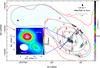 |
Fig. 1 IRAM/PdBI 3 mm continuum image of the W43-MM1 ridge, revealing a cluster of MDCs. The black dashed contour outlines the area where the confidence-weight map exceeds 90%. Column densities yielded by Herschel imaging (see Nguyen Luong et al. 2013) and shown in red contours are used to define A–D subregions. The black dotted-dashed line and the 1023 cm-2 contour outline the eastern and western parts of the ridge. Black and white ellipses plus numbers locate MDCs extracted by Getsources (see Table 2), the green ellipse outlines N12, and the black asterisk pinpoints a source identified by Beuther et al. (2012). Negative contours have been removed to reduce confusion. See Fig. 6 for the version with negative contours. Zoom inset: IRAM/PdBI 1 mm continuum image of the W43-N1 MDC. Black ellipses are HMPCs extracted by Getsources (see Table 2). |
A seven-field 3 mm mosaic of the W43-MM1 ridge and a single 1 mm pointing toward W43-N1, its most massive dense core, were carried out with the IRAM Plateau de Bure Interferometer (hereafter IRAM/PdBI, see Table 1). Configurations C2 and D with four and six antennas, respectively, were used in March–April and October–November 2002 for the single pointing toward the phase center (α,δ) = 18:47:47.1, −01:54:28; configurations C and D were used in October and July 2011 with respectively five and six antennas for the mosaic. Broad-band continuum and spectral lines (not shown here) were simultaneously observed. The phase, amplitude, and correlator bandpass were calibrated on strong quasars (3C 273, 4C 09.57, and 1936-155 in 2002; 3C 454.3, 1827+062, and 0215+015 in 2011), while the absolute flux density scale was derived from MWC349 observations. The absolute flux calibration uncertainty is estimated to be ~15%.
The two WIDEX subunits were combined to observe the continuum emission with a total bandwidth of 3.6 GHz centered at 87.5 GHz (3 mm). Two correlator units were summed into a 640 MHz bandwidth centered at 239.5 GHz (1 mm). The mean angular resolutions were respectively  at 3 mm and
  at 1 mm.
We used the GILDAS2 package to calibrate each dataset, merge the visibility data of all fields for the 3 mm mosaic, then invert and clean (natural cleaning) both the 1 mm and 3 mm. We built a “pure” continuum map at 3 mm from spectral bands of WIDEX free of strong lines. The 3 mm continuum map is given in Fig. 1. It displays a very inhomogeneous repartition of the continuum with much more emission in the southwestern part of the map. Owing to limited dynamic range around the strong continuum and extended source W43-N1, we obtain significantly different rms levels in the northeastern part of the 3 mm mosaic (3σ ~ 0.11 mJy/beam) than in the southern region around W43-N1 (3σ ~ 3.8 mJy/beam). As for the 1 mm pointing, we measured a 3σ rms level of ~0.15 Jy/beam.
2.2. Herschel dust temperature and column density maps
We used the dust temperature and column density images built from Hi-GAL and HOBYS data (Molinari et al. 2010; Motte et al. 2010) and presented by Nguyen Luong et al. (2013). Using three of the four longest wavelengths of Herschel (160–350 μm), they derived the total (gas+dust) column density (NH2) and average dust temperature maps of W43-Main with an angular resolution of 25″ (see Table 1). Following the procedure fully described in Hill et al. (2011, 2012), they fitted pixel-by-pixel spectral energy distributions (SEDs) with modified blackbody models. They used a dust opacity law similar to that of Hildebrand (1983) but with β = 2 instead of β = 1 and assumed a gas-to-dust ratio of 100: κν = 0.1 × (300 μm /λ)2 cm2 g-1. It provides column density images with very low (20% when Av> 10 mag) relative uncertainties, arising from SED fit errors (Hill et al. 2009) and possible variations in the emissivity index through the map. The absolute accuracy of Herschel NH2 maps has been estimated to be around 40% (Roy et al. 2014).
3. MDCs census in the W43-MM1 ridge
MDC and HMPC samples.
To extract the MDCs, we used the source extraction tool Getsources (Men’shchikov et al. 2012). Developed for multiwavelength Herschel images, it calculates the local noise and local background to properly extract compact sources from a complex cloud environment. We increased the quality constraints3 of Getsources to account for the specificity of our interferometric images. To perform a confident extraction of MDCs, we masked the map borders where confidence map weights drop below 10% (dashed contour in Fig. 1). We also set a maximum source size of 0.25 pc to focus on 0.1 pc MDCs at 3 mm, and 0.02 pc at 1 mm to focus on 0.01 pc high-mass protostellar cores (HMPCs).
At 3 mm, Getsources identified 11 MDCs, with average deconvolved sizes of ~0.07 pc, all located in the densest southwestern part of the W43-MM1 ridge (see Fig. 1 and Table 2). Four MDCs are substructures of ~0.2 pc clumps extracted by Motte et al. (2003) and four correspond to the ~0.02 pc HMPCs identified by Sridharan et al. (2014). Among our MDCs, six have outflows (Louvet et al., in prep.). Only N12, the least massive of our sample (~20 M⊙), was suggested by outflows but not extracted by Getsources. Beuther et al. (2012) detected another diffuse dust source of ~30′′ size that remains undetected (see Fig. 1), likely filtered out by the interferometer (filtering scale ~20′′). The map shown in Fig. 1 suggests an uneven distribution of the dense gas, with three MDCs forming in the eastern part of the ridge and eight MDCs in its western part.
The 1 mm map only covers the W43-N1 MDC (see Fig. 1). It shows that this core splits into two HMPCs (see Fig. 1 and Table 2) with sizes approaching that of protostellar envelope scales (e.g., Rathborne et al. 2007; Bontemps et al. 2010).
To derive the masses of the MDCs in our sample, we assumed that the 3 mm continuum emission mainly arises from thermal dust and is optically thin. The free-free contribution to the 3 mm fluxes is estimated to be much less than 20% for the MDCs. Indeed, the noise peaks found in the Cornish survey at 2 cm (Hoare et al. 2012) and extrapolated at 3.4 mm assuming an optically thin free-free emission spectral index correspond to a free-free contamination of ~0% for most MDCs up to ~20% for N7.
The MDC masses are calculated from the integrated fluxes measured by Getsources,  , via
, via 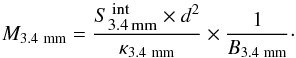 with d the distance from the Sun and B3.4 mm(Tdust) the Planck function. The dust mass opacity was taken to be equal to κ3.4 mm = 2.6 × 10⁻³ cm2 g-1, following the κν = 0.1 cm2 g-1 × (ν/ 1000 GHz)β equation with an opacity index β = 1.5, which is typical of dense and cool media (Ossenkopf & Henning 1994).
We used Tdust = 20 K as suggested by the averaged Herschel dust-temperature map over the W43-MM1 ridge (see Sect. 2) and the dust temperature estimated for the W43-MM1 clump alone (Motte et al. 2003; Bally et al. 2010). The formula results in 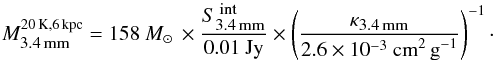 (1)Errors on the
  masses mostly arise from the dust mass opacity at 3.4 mm, which could be a factor 3.5 smaller, if one uses an optical index of β = 2, thus increasing the masses by a similar factor. Moreover, since N1 hosts a hot core (e.g. Herpin et al. 2012; Sridharan et al. 2014), its temperature could be higher than 20 K. The temperature constraints presented in Motte et al. (2003) and Sridharan et al. (2014), namely 20 K and 300 K for a full width half maximum (FWHM) of 0.25 pc and 0.017 pc, respectively, suggest a temperature profile of T ∝ FWHM-1. This would leads to a temperature of 55 K for the N1 MDC, and would decrease its mass down by a factor of 3.
The masses of HMPCs at 1.3 mm (see Table 2) were calculated from an equivalent equation to Eq. (1) at 1.3 mm, using κ1.3 mm = 0.01 cm2 g-1. The dust opacity uncertainties could contribute to errors on the mass measurements up to a factor 2. Application of the temperature profile derived above (T ∝ FWHM-1) would decrease the 1.3 mm mass of N1a by a factor of 10.
Following the above assumptions on κ and T = 20 K, we recalculated the published masses of a few MDC and protostar samples (Beuther et al. 2002; Rathborne et al. 2007; Motte et al. 2007; Bontemps et al. 2010; Peretto et al. 2013; Wang et al. 2014) to make meaningful comparisons with the present study (see Table 2 and Fig. 2). Because of obvious spatial resolution constraints, most searches for high-mass protostars focused on <3.5 kpc regions. We recall that, at these close distances from the Sun, the richest high-mass star-forming region is Cygnus X (see Kryukova et al. 2014, and references therein).
W43-MM1 MDCs have radii that are twice smaller than those found in the MDCs of Cygnus X (Motte et al. 2007), and they are ten times denser (see Table 2). As shown in Fig. 2, W43 MDCs lie above the general correlation of density versus radius found for samples of MDCs (Motte et al. 2007) and HMPCs (e.g., Rathborne et al. 2007; Peretto et al. 2013; Wang et al. 2014).
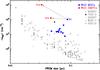 |
Fig. 2 Comparison of density to radius of the W43 MDCs (massive dense cores) and HMPCs (high-mass protostellar cores) with the sources presented in Motte et al. (2007), Rathborne et al. (2007), Bontemps et al. (2010), Peretto et al. (2013), and Wang et al. (2014). The W43 MDCs and HMPCs lie above the general trend, and with respect to their sizes, they are the densest cloud structures. |
Physical properties in subregionsa of W43-MM1.
Special case of the remarkable objects N1a and N1b
It is statistically understandable to find the most extreme objects in W43, since it is one of the most massive and most concentrated cloud complexes of the Milky Way (Nguyen Luong et al. 2011b). Nevertheless, we stress the remarkable N1a and N1b HMPCs extracted at 1 mm, which are ~1100 M⊙ and ~400 M⊙, respectively, gathering together 70% of the N1 MDC mass measured at 3 mm. Their masses are consistent with those measured by Sridharan et al. (2014) when the difference in spatial resolution, dust mass opacity, and temperature are accounted for. These two HMPCs are a factor 30–90 as massive as those found in Cygnus X (see Table 2 and Fig. 2). They look even more exceptional compared to the high-mass protostars studied by Wang et al. (2014) (see Table 2).
N1a is even three times more massive and 15 times denser than the SDC335-MM1 HMPC (Peretto et al. 2013) (see Table 2). Remarkably, N1a is still in its earliest phase of evolution since it is only associated with weak mid-infrared emission (Motte et al. 2003). Given its mass and following the definition of Motte et al. (2007), N1a should host the most massive protostar known in the IR-quiet phase, i.e., before a >8 M⊙ embryo has formed.
4. Core formation efficiency of W43-MM1
We divided the ridge into four subregions A, B, C, and D (see Fig. 1). Assuming4cs ≃ 0.2 km s-1, they are spaced from one another by more than five crossing lengths. This ensures that one generation of protostars takes place before MDCs change subregion. Translated in terms of column density, this leads to subregion A having NH2> 3.5 × 1023 cm-2. Subregions B, C, and D are then shells associated with the annular areas where NH2∈[1.75 − 3.5], NH2∈[1 − 1.75] × 1023 cm-2, and NH2<1023 cm-2, respectively. We hereafter define the CFE as the ability to concentrate pc3 clouds with nH2 ~ 104 cm-3 density into high-density seeds of ~10-3 pc3 and nH2 ~ 107 cm-3. This CFE connects those measured for 100 pc cloud complex to 1 pc clumps (e.g., Nguyen Luong et al. 2011a; Eden et al. 2012) to those for 0.1 pc MDCs to 0.01 pc protostars (e.g., Motte et al. 1998; Bontemps et al. 2010; Palau et al. 2013). We calculated the CFE as  , which is the ratio of the gas mass within MDCs over the subregion cloud mass.
The total mass of MDCs in each subregion,  , was computed from the masses derived for MDCs extracted by Getsources, as explained in Sect. 3 (see Table 2). The repartition of cores in the subregions A, B, C and D assumes that there are no projection effects, i.e., for instance, N9 belongs to B, not C or D. To check the robustness of this assumption, we made tests randomly distributing MDCs in the different subregions. When N5, N7, and N11 MDCs, which should logically cluster in the high-density medium of subregion A, are located within subregion B, CFEs of A and B become 31% and 15%, respectively. Thus, as long as the most massive MDCs N1 and N2 belong to subregion A, the slope index of the correlation discussed below between the CFE and the density changes by less than 20%.
The cloud masses, Mcloud (see Table 3), were derived from the Herschel column density map, after subtracting the 4 × 1022 cm-2 background level defined as in Nguyen Luong et al. (2013). To derive cloud densities, we had to define the 3D geometry of the subregions. Subregions are separated shells, in the sense that region B does not include region A, etc. Subregion A was taken to be a sphere of radius 0.53 pc. The subregions sums A+B, A+B+C, and A+B+C+D are assumed to be ellipsoids with major axes in pc of 1.6 × 1.6 × 2.3, 2 × 2 × 3.9 and 2.1 × 2.1 × 4.6, respectively. For instance, the volume of region B, VB, is then VA+B-V pc3. The relative uncertainties for volume densities of subregions A–D should be negligible and are not reported in Figs. 3–4. The absolute errors for cloud densities are ~50%, taking absolute uncertainties of ~40% for the cloud masses and 30% error on cloud volumes due to line-of-sight effects into account.
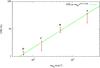 |
Fig. 3 Linear correlation of the core formation efficiency from pc3 clouds to 10-3 pc3 dense cores with the cloud volume density. Relative uncertainties are estimated from error measures on MDCs masses, and the green line is the power-law fit to these four points corresponding to subregions A–D. |
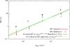 |
Fig. 4 Linear dependence of the star formation efficiency in subregions A–D on cloud volume density. The red points and error bars correspond to the first approach explained in Sect. 5 to derive the SFEs and blue points to the second. The green line is the linear fit to the first approach and the brown line the relation of Bonnell et al. (2011). |
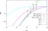 |
Fig. 5 SFR estimates over W43-MM1 compared to the multifreefall extrapolation of models from Krumholz & McKee (2005), Padoan & Nordlund (2011), and Hennebelle & Chabrier (2011), given in Federrath & Klessen (2012) and a magnetized model from Hennebelle & Chabrier (2013) (blue, pink, cyan, and black curves, respectively). The analytic models struggle to reproduce the observed SFRff (red errorbars, blue stars and green line) at low αvir. |
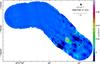 |
Fig. 6 IRAM/PdBI 3 mm continuum image of the W43-MM1 ridge. The black dashed contour delimits the area where the confidence map exceeds 10%. Black and white ellipses plus numbers locate MDCs extracted by Getsources. |
Figure 3 displays the CFE measured for regions A–D as a function of their mean density. Relative uncertainties on the CFEs are only two to 15%, since they only depend on the quality of the MDCs extraction. In contrast, absolute uncertainties could be as high as a factor of 4. This mostly comes from the combined inaccuracies of the dust mass emissivity both at Herschel and 3.4 mm wavelengths. In Figs. 3–5, we only consider relative uncertainties, since we hereafter mainly discuss the relative behavior of the CFE (resp. the SFE) as a function of the cloud density. Figure 3 reveals a clear correlation between the CFE and the cloud density, represented well by CFE  . This slope has to be considered as a lower limit since the noise level of the 3.4 mm map increases toward its central part (i.e., from D to A), decreasing our MDC detection capabilities. With the relative CFE uncertainties and projection effects described above, the slope is uncertain by 5% and 20%, respectively.
Palau et al. (2013) studied the fragmentation of a few ~0.1 pc MDCs into ~0.01 pc protostars. They gathered results from many other high-resolution millimeter studies and plotted the CFE against volume density. Their Fig. 6 displays the same trend as our W43-MM1 observations. The ability to concentrate gas thus seems to increase with density for the cloud scale of 1–10 pc, as well as the dense core scale of 0.1 pc, and possibly regardless of the physical scale considered.
5. Star formation efficiency and star formation rate
5.1. The instantaneous SFE and SFR
We used the MDCs census from Sect. 3 to estimate the SFE and the SFR (see also Motte et al. 2003; Nguyen Luong et al. 2011a; Nguyen Luong 2012). The SFE is the ratio of the total mass of stars forming, M⋆, to the cloud mass Mcloud (see Table 3): SFE = M⋆/Mcloud. The star formation rate itself is the ratio of stellar mass, M⋆, to the age of the star formation event considered. We used a mean protostellar lifetime of ~0.2 Myr (Russeil et al. 2010; Duarte-Cabral et al. 2013) to derive the SFRs.
The above calculations give access to the “instantaneous” SFEs and SFRs. Indeed, the counting of protostars in each MDC should provide a direct measurement of star formation occurring in a cloud during one generation of protostars. It is especially adequate for ridges, which are forced-falling clouds (see Schneider et al. 2010; Nguyen Luong et al. 2013). This contrasts with counts of Spitzer young stellar objects in nearby clouds (e.g., Heiderman et al. 2010), which compare the mass of already formed young stellar objects to the mass of a cloud forming a new generation of stars, assuming a continuous star formation over 2 Myr. These counts provide, by analogy, the “integrated” SFE and SFR.
5.2. Calculation approaches
The main difficulty encountered when estimating the instantaneous SFEs and SFRs is defining the total mass of forming stars, M⋆, in each dense core. We estimated M⋆, hence the SFEs and SFRs, using two approaches. The first one simply assumes that a constant efficiency from MDC to stellar cluster, ϵ, is suitable for MDCs. The second one is based on an estimate of the most massive star each MDC can form, which is extrapolated to a protostellar cluster mass using the stellar initial mass function (IMF).
For the first approach in estimating M⋆, a “MDC-to-stellar cluster” efficiency of ϵ = 30% was assumed in the relation  . On small scales, this core efficiency is generally assumed to be constant regardless of the core mass (e.g., Alves et al. 2007). This efficiency bridges the value estimated for the Cygnus X MDCs (40% in Bontemps et al. 2010) and those measured for the lower mass ρ Oph dense cores (5 − 35% in Motte et al. 1998). It also recalls the efficiency measured by comparing the core mass function of low-mass star-forming regions to the IMF (ϵ = 30% according to Alves et al. 2007; André et al. 2010). This approach directly relates the CFEs measured in Sect. 4 to the SFEs by SFE-Method1 = ϵ× CFE. It is based on the assumption that ϵ does not depend on the MDC density, which is questionable according to, say, Palau et al. (2013, and references therein).
The second approach follows the finding of Bontemps et al. (2010) that Cygnus X MDCs, which weigh ~60 M⊙ within 0.1 pc, form on average two (± 1) 8 M⊙ protostars. To be conservative, we assumed that MDCs less massive than 200 M⊙ would form only one 8 M⊙ protostar, along with its associated cluster. For cores N2 and N3, which are more massive than 200 M⊙, they should be able to form at least one 50 M⊙ star, given the result of Peretto et al. (2013). In the particular case of N1, the 1 mm data at 2 2 show a fragmentation into two ~0.04 pc cores, N1a and N1b. Each of them is above 200 M⊙, we therefore assumed that N1 would form two stars of 50 M⊙ and their associated clusters.
From these estimations of the most massive star forming in each MDC, we calculated the total stellar mass, M⋆ (see Table 3), applying the canonical IMF description of Kroupa (2001)5. For this, we assumed that the IMF distribution applies to each subregion. It assumes that the detected MDCs along with the undetected lower mass ones display a CMF that will correctly sample the IMF. The IMF was integrated from the brown dwarf limit of 0.08 M⊙ to 150 M⊙ (Martins et al. 2008; Schnurr et al. 2008), leading to a fraction of stellar mass within high–mass (>8 M⊙) stars of ~22%. The choice of 150 M⊙ for the upper limit has little impact on this stellar fraction, and a choice of 300 M⊙ for instance (see Crowther et al. 2010) would lead to a stellar fraction within high-mass stars of ~25%.
Given the assumptions associated with these two approaches, the SFE and SFR values we derived are consistent with each other. They agree within factors of 1.15 to 2 (see Table 3). The main limitation of the first method is the assumption that no star forms outside the detected MDCs. As for the second method, the limitation comes from the applicability of the IMF to each subregion. The relative and absolute uncertainties of the SFEs and the SFRs mostly arise from uncertainties on CFEs (see Sect. 4) and protostellar lifetime. We estimate relative uncertainties to be 20% and 40% and absolute ones to be four and ten for the SFEs and the SFRs, respectively.
Subregion properties to be compared to SFR statistical models.
5.3. SFE relation with cloud density
Figure 4 displays the SFE estimated through both approaches as a function of the cloud volume density for the four subregions A–D. The correlation found between the CFE and density is retrieved for the SFE:  . It obviously comes from the linear relation taken for the first approach, but it validates the SFE values of the second approach, for which we fit SFE-Approach2
 .
.
We then aim to compare the observed SFEs versus ⟨ nH2 ⟩ cloud relation with those predicted by models. There is a lack of published plots that could be compared to our Fig. 4. We thus investigated the recent numerical simulations by Bonnell et al. (2011), whose cloud mass and size, as well as fragmentation resolution, suit our present study. They simulated a 104 M⊙, 10 pc elongated molecular cloud, initially marginally unbound due to turbulence, but with the high-mass star-forming region centered on the part of the cloud that is gravitationally bound. Sink particles are used to follow regions of gravitational collapse over densities of 1.7 × 1010 cm-3 and sizes <0.001 pc. We investigated the behavior of the SFE within shells around clumps against density and found a relation close to SFE ∝ for 100 − 2 × 105cm-3 densities (see Fig. 7). Astonishingly, this SFE relation is extremely close to the observed one, and it clearly increases with density. A similarly good correlation is found with volume density for the SFE measured within clumps rather than shells. This behavior contrasts with past cloud-scale studies of the SFR (Evans et al. 2009; Lada et al. 2010). Indeed, they suggest a linear correlation, in log-log space, with the mass of the cloud above an Av threshold, rather than its density (see, however, Gutermuth et al. 2011).
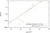 |
Fig. 7 Efficiency of core formation measured as the fraction of mass that is inside the SPH sink particles as a function of the cloud gas density (extrapolated from Bonnell et al. 2011). Both the efficiency and the gas densities are measured in spherical shells centered on the densest region of the simulation and span size scales from ~ 0.04 to 10 pc. The points represent regions where the sink particles are all between 40 000 and 100 000 years old. The efficiencies increase with time such that older systems would have higher efficiencies, but the relation between SFE and ⟨ nH2 ⟩ remains. |
5.4. SFE/SFR absolute values
The SFEs obtained for the W43-MM1 ridge and its subregions A and B are large, SFEs = 3 − 11%, and their SFRs estimates are 4–11 larger than the values predicted, given the subregion masses, by the simple equation proposed by Lada et al. (2013). Our estimations of the SFE and of the SFR over the ridge confirm its ability to form a rich cluster of massive stars: SFE = 6% and SFR = 6000 M⊙ Myr-1 over only a 8 pc3 volume. These values are reminiscent of those found, on larger physical and time scales, for starburst galaxies (see e.g., Kennicutt 1998). As already noted by Motte et al. (2003), the W43-MM1 ridge qualifies as a ministarburst region. As in the case of the G035.39–00.33 ridge (Nguyen Luong et al. 2011a), both fragmentation and stellar formation are efficient in the high-density regions forming the W43-MM1 ridge. The absolute value of the SFR of the W43-MM1 ridge has to be taken with caution owing to the numerous uncertainties, but it may account for one twentieth of the total ~1 M⊙ yr-1 SFR of the Milky Way, during one protostellar lifetime of ~0.2 Myr.
A closer inspection of star formation activity between the eastern and the western parts of the ridge reveals a clear disparity (see Fig. 1 and Table 3). Even though they have similar masses, the SFE and the SFR in the western part are about twenty times greater than in the eastern one (10.2% versus 0.6%). With a microturbulent support alone, the cloud of the eastern ridge would instantly fragment and form stars. However, the W43-MM1 ridge is constituted of several gas flows/filaments that are supersonically merging (Louvet et al., in prep.) and developing shears and low-velocity shocks (Nguyen Luong et al. 2013). The observed SFE disparity is thus coherent with the western part of the ridge having already formed a protostellar cluster (see Fig. 1) and its eastern part still being assembling material (Louvet et al., in prep.).
6. Comparison to statistical models of star formation rate
The SFR statistical models are analytic descriptions of a turbulent cloud that include magnetized turbulence and self-gravity, which acts as a filter to select the core progenitors (Krumholz & McKee 2005; Padoan & Nordlund 2011; Hennebelle & Chabrier 2013). They are based on the integration of the density probability distribution function (PDF), which is assumed to be a log-normal distribution. In the simplest approach, the density PDF is weighted by the free-fall time and integrated above a certain density threshold. Therefore, the different models differ by the density threshold that is chosen in the integration of the PDF (see e.g., Hennebelle & Chabrier 2011; Federrath & Klessen 2012). However in practice, while reasonable, this approach does not take the complex and heterogeneous spatial distribution of the gas into account. Moreover, it is rather unclear that simple thresholds, based for example on mean Jeans mass, are justified since the density varies over orders of magnitude. A different type of approach is the calculations performed by Hennebelle & Chabrier (2011, 2013) (see also multifreefall extrapolations of SFR models by Federrath & Klessen 2012). They use the multiscale method developed in cosmology (Press & Schechter 1974) and take the gas spatial distribution characterized by a power spectrum into account. If the density variance is of independent scale, it is equivalent to the PDF integration approach described above. Due to our lack of knowledge in the exact statistics of molecular clouds, in particular how to define their boundaries, this approach is also hampered by large uncertainties.
To infer a dimensionless star formation rate independent of the cloud mass and density, SFRff (Krumholz & McKee 2005), the following normalized quantity has been defined:  (2)The freefall times,
  and
and  , are estimated from the mean cloud and mean MDCs densities respectively via
  (3)where G is the gravitational constant and ρ the cloud or MDCs gas density.
Usually, models plot the SFRff as a function of the virial parameter, αvir = 2Ekin/ | Egrav | = σ2 × Rcloud × 5/(3 × G × Mcloud) because they are two normalized quantities. We thus computed the freefall times of all subregions A–D, plus the mean freefall time of the MDCs they host (see Table 4). We estimated αvir for all subregions6 (see Fig. 1 and Table 4), using a turbulence velocity of σ = 2.2 km s-1 (Nguyen Luong et al. 2013) adequate for the complete W43-MM1 ridge. We calculated the SFRff for the two approaches (see Table 4) presented in Sect. 5. We selected models of Mach number equal to 9.5 and parameters proposed in Federrath & Klessen (2012)7. As described above, these three models integrate the density PDF and differ by the density thresholds. The model labeled KM05 uses the sonic length, i.e., the length at which velocity dispersion and sound speed are equal, and requires that the Jeans length be less that its value. The model labeled PN11 requires that the Jeans length must be less than the typical size of the shocked layer, while the model labeled HC11 simply states that the integration should be performed over all pieces of gas whose densities are such that the associated Jeans length is less than a fraction of the cloud size. Second, since a significant magnetic field has been measured toward W43-MM1 (mass-to-flux ratio ~2, Cortes et al. 2010), we also present a magnetic model taken from Hennebelle & Chabrier (2013). A magnetic field of 20 μG ×(nH2/ 103 cm-3)0.3 is assumed for this model. These values are reasonable given what is known on the magnetic field in this region (Cortes et al. 2010). Their exact choice, at this stage, is dictated by the reasonable agreement with the data on the SFR.
Before comparing our results with the models, we would like to stress that all models have similar behaviors. Indeed, for extremely cold clouds (i.e., have low α), most of the gas is gravitationally unstable, and therefore a significant fraction of the density PDF contributes in the integration. Since it is normalized by the total mass and mean freefall time, the SFR tends toward a constant value which is on order of ϵ. However, because the density PDF is weighted by the freefall time, which is shorter at high densities, the normalized SFR can be larger than ϵ, here taken to be 30%. For clouds that are supported more against gravity, only the densest regions contribute to star formation. Thus only the high-density part of the PDF contributes. This leads to a SFR that can be arbitrarily low and can have a stiff dependence on the cloud parameters.
Figure 5 displays our SFRff estimates against αvir along with the multifreefall extrapolation of isothermal models from Krumholz & McKee (2005) and Padoan & Nordlund (2011) computed by Federrath & Klessen (2012), plus the magnetized model exposed in Hennebelle & Chabrier (2013). As in models, the observed SFRff relation at high αvir increases with decreasing virial parameter αvir and its dependence index recalls the one of models at high αvir (see Fig. 5). But, none of the models can correctly describe the observations at low αvir (<0.2). Indeed, all models depart from the αvir-dependent regime to join the saturation regime, while observations still seem to be anti-correlated to αvir. We nevertheless note the HC13 model is in better agreement and that the second approach in estimating SFRff has a trend closer to the model behavior.
Both theories and observations need to go one step further to solving this question. For theories, the difference in behavior could be understood when recalling that ridges do not fit two major hypotheses of these analytic models. Ridges first represent column density points that depart from the log-normal distribution assumed in all models (Hill et al. 2011). Second, these regions are forced-falling clouds whose turbulence level probably does not follow the Larson law used in the SFRff models (Schneider et al. 2010; Nguyen Luong et al. 2013). Combined, these two reasons could explain why, in gravity-dominated regions, the current SFRff models cannot apply in their present formulation. From the observational side, a higher resolution and deeper imaging are needed to estimate robust SFR values from a complete census of high- to low-mass protostellar cores.
7. Conclusion
We used the IRAM Plateau de Bure interferometer to image the W43-MM1 ridge at 3 mm and a zoom on its main MDC at 1 mm (see Fig. 1). We compared the mass distribution observed throughout these maps with the column density image of W43-MM1 built from Herschel data. Our main results and conclusions may be summarized as follows
-
The 3 mm mosaic reveals eleven~0.07 pc MDCs, labeled N1 to N11, acrossthe W43-MM1 ridge. These MDCs range in mass between~50 M⊙ and ~2100 M⊙ and have meandensities between nH2~ 7× 106 cm-3 and ~1× 108 cm-3.The 1 mm snapshot identifiestwo ~0.03–0.04 pc HMPCs within N1, the mostmassive of the MDCs sample (see Table 1). TheN1a protostellar core, with its ~1080 M⊙ mass, is themost massive known 0.03 pc young stellar ob-ject ever observed in an early phase of evolution (see Fig. 2). It isexpected to form a couple of ~50 M⊙ stars.
-
We used the MDCs masses to estimate the concentration of the cloud gas toward high density (see Table 3), usually called the gas-to-core formation efficiency (CFE). The W43-MM1 ridge split into four exclusive subregions displays a clear correlation of the CFE with cloud volume density: CFE
 (see Fig. 3).
 -
The CFE measurements were extrapolated to “instantaneous” stellar formation efficiencies (SFEs) following two approaches constraining the MDC to stellar cluster efficiency (see Table 3 and Fig. 4). The SFE values were also used to estimate 1) the “instantaneous” stellar formation rate (SFR) expected during the protostellar lifetime and 2) the dimensionless SFR per free-fall time theoreticians use: SFRff.
-
The SFEs obtained for the W43-MM1 ridge and its subregions A and B are high, SFEs = 3–11%, and their SFRs estimates are 4 to 11 times larger than the values expected from their masses, following the equation proposed by Lada et al. (2013). We propose that it is due to a strong correlation of the CFE to the gas volume densities in W43-MM1. With its SFR absolute value, SFR = 6000 M⊙ Myr-1, W43-MM1 qualifies as a ministarburst region. During one protostellar lifetime of ~0.2 Myr, it may account for as much as one twentieth of the total ~1 M⊙ yr-1 SFR of the Milky Way.
-
The CFE of the eastern and western parts of the ridge are clearly unbalanced, leading to SFE values as different as 0.6% and 10.2%. It might be due to the eastern region currently assembling its mass along multiple filaments whose interaction could impede cloud fragmentation and star formation.
-
Our observations lead to a SFRff relation with a virial number that is steadily increasing when αvir is decreasing (see Fig. 5). While statistical SFR models display such a trend for high αvir, they saturate for values close to those observed in the W43-MM1 ridge. Models with more realistic conditions are needed to fully describe the complexity of this very dense, turbulent, nonisothermal, and nonstationary cloud structure. Higher resolution and deeper imaging are necessary to confirm current observational findings.
Based on observations carried out with the IRAM Plateau de Bure Interferometer. IRAM is supported by INSU/CNRS (France), MPG (Germany), and the IGN (Spain).
The Grenoble Image and Line Data Analysis Software is developed and maintained by IRAM to reduce and analyze data obtained with the 30 m telescope and Plateau de Bure interferometer. See www.iram.fr/IRAMFR/GILDAS
Input parameters “sreliable” and “cleantuning” were multiplied by two with respect to the default values of Getsources. The parameter “sreliable” controls the significance of reliable sources in the extraction catalogs and the parameter “cleantuning” adjusts the cleaning depth.
The σ ~ 2.2. km s-1 turbulent velocity measured by Nguyen Luong et al. (2013) cannot be used to estimate the crossing length since line widths in this region do not trace microturbulent motions but do trace organized flows building the ridge (Louvet et al., in prep.).
Kroupa (2001) describes the stellar IMF with a two-part power law: ξ(m) ∝ m− αi with αi = 1.3 for m ∈ [0.08,0.5] M⊙ and αi = 2.3 for m ∈ [0.5, ∞[M⊙.
The radii of subregions B–D are estimated from spheres with volumes equal to VB, VC and VD respectively.
The forcing parameter, b, is set to 0.4; the magnetic field is not taken into account (β → ∞).
Acknowledgments
We thank Christoph Federrath for the fruitful discussions we had on SFR. We are grateful to Alexander Men’shchikov for help in customizing Getsources for interferometric images.
References
- Alves, J., Lombardi, M., & Lada, C. J. 2007, A&A, 462, L17 [NASA ADS] [CrossRef] [EDP Sciences] [Google Scholar]
- André, P., Men’shchikov, A., Bontemps, S., et al. 2010, A&A, 518, L102 [NASA ADS] [CrossRef] [EDP Sciences] [Google Scholar]
- Bally, J., Anderson, L. D., Battersby, C., et al. 2010, A&A, 518, L90 [Google Scholar]
- Beuther, H., Schilke, P., Menten, K. M., et al. 2002, ApJ, 566, 945 [NASA ADS] [CrossRef] [Google Scholar]
- Beuther, H., Tackenberg, J., Linz, H., et al. 2012, A&A, 538, A11 [NASA ADS] [CrossRef] [EDP Sciences] [Google Scholar]
- Bonnell, I. A., Smith, R. J., Clark, P. C., & Bate, M. R. 2011, MNRAS, 410, 2339 [NASA ADS] [CrossRef] [Google Scholar]
- Bontemps, S., Motte, F., Csengeri, T., & Schneider, N. 2010, A&A, 524, A18 [NASA ADS] [CrossRef] [EDP Sciences] [Google Scholar]
- Carlhoff, P., Nguyen Luong, Q., Schilke, P., et al. 2013, A&A, 560, A24 [NASA ADS] [CrossRef] [EDP Sciences] [Google Scholar]
- Cortes, P., & Crutcher, R. M. 2006, ApJ, 639, 965 [Google Scholar]
- Cortes, P. C., Parra, R., Cortes, J. R., & Hardy, E. 2010, A&A, 519, A35 [NASA ADS] [CrossRef] [EDP Sciences] [Google Scholar]
- Crowther, P. A., Schnurr, O., Hirschi, R., et al. 2010, MNRAS, 408, 731 [NASA ADS] [CrossRef] [Google Scholar]
- Csengeri, T., Bontemps, S., Schneider, N., Motte, F., & Dib, S. 2011, A&A, 527, A135 [NASA ADS] [CrossRef] [EDP Sciences] [Google Scholar]
- Duarte-Cabral, A., Bontemps, S., Motte, F., et al. 2013, A&A, 558, A125 [NASA ADS] [CrossRef] [EDP Sciences] [Google Scholar]
- Eden, D. J., Moore, T. J. T., Plume, R., & Morgan, L. K. 2012, MNRAS, 422, 3178 [NASA ADS] [CrossRef] [Google Scholar]
- Evans, II, N. J., Dunham, M. M., Jørgensen, J. K., et al. 2009, ApJS, 181, 321 [NASA ADS] [CrossRef] [Google Scholar]
- Evans, II, N. J., Heiderman, A., & Vutisalchavakul, N. 2014, ApJ, 782, 114 [NASA ADS] [CrossRef] [Google Scholar]
- Federrath, C., & Klessen, R. S. 2012, ApJ, 761, 156 [NASA ADS] [CrossRef] [Google Scholar]
- Gutermuth, R. A., Pipher, J. L., Megeath, S. T., et al. 2011, ApJ, 739, 84 [NASA ADS] [CrossRef] [Google Scholar]
- Heiderman, A., Evans, II, N. J., Allen, L. E., Huard, T., & Heyer, M. 2010, ApJ, 723, 1019 [NASA ADS] [CrossRef] [Google Scholar]
- Hennebelle, P., & Chabrier, G. 2011, ApJ, 743, L29 [NASA ADS] [CrossRef] [Google Scholar]
- Hennebelle, P., & Chabrier, G. 2013, ApJ, 770, 150 [NASA ADS] [CrossRef] [Google Scholar]
- Hennemann, M., Motte, F., Schneider, N., et al. 2012, A&A, 543, L3 [NASA ADS] [CrossRef] [EDP Sciences] [Google Scholar]
- Herpin, F., Chavarría, L., van der Tak, F., et al. 2012, A&A, 542, A76 [NASA ADS] [CrossRef] [EDP Sciences] [Google Scholar]
- Hildebrand, R. H. 1983, QJRAS, 24, 267 [NASA ADS] [Google Scholar]
- Hill, T., Pinte, C., Minier, V., Burton, M. G., & Cunningham, M. R. 2009, MNRAS, 392, 768 [NASA ADS] [CrossRef] [Google Scholar]
- Hill, T., Motte, F., Didelon, P., et al. 2011, A&A, 533, A94 [NASA ADS] [CrossRef] [EDP Sciences] [Google Scholar]
- Hill, T., Motte, F., Didelon, P., et al. 2012, A&A, 542, A114 [NASA ADS] [CrossRef] [EDP Sciences] [Google Scholar]
- Hoare, M. G., Purcell, C. R., Churchwell, E. B., et al. 2012, PASP, 124, 939 [NASA ADS] [CrossRef] [Google Scholar]
- Kennicutt, Jr., R. C. 1998, ApJ, 498, 541 [NASA ADS] [CrossRef] [Google Scholar]
- Kroupa, P. 2001, MNRAS, 322, 231 [NASA ADS] [CrossRef] [Google Scholar]
- Krumholz, M. R., & McKee, C. F. 2005, ApJ, 630, 250 [NASA ADS] [CrossRef] [Google Scholar]
- Kryukova, E., Megeath, S. T., Hora, J. L., et al. 2014, AJ, 148, 11 [NASA ADS] [CrossRef] [Google Scholar]
- Lada, C. J., Lombardi, M., & Alves, J. F. 2010, ApJ, 724, 687 [NASA ADS] [CrossRef] [Google Scholar]
- Lada, C. J., Lombardi, M., Roman-Zuniga, C., Forbrich, J., & Alves, J. F. 2013, ApJ, 778, 133 [NASA ADS] [CrossRef] [Google Scholar]
- Martins, F., Hillier, D. J., Paumard, T., et al. 2008, A&A, 478, 219 [NASA ADS] [CrossRef] [EDP Sciences] [Google Scholar]
- Men’shchikov, A., André, P., Didelon, P., et al. 2012, A&A, 542, A81 [NASA ADS] [CrossRef] [EDP Sciences] [Google Scholar]
- Molinari, S., Swinyard, B., Bally, J., et al. 2010, A&A, 518, L100 [NASA ADS] [CrossRef] [EDP Sciences] [Google Scholar]
- Motte, F., Andre, P., & Neri, R. 1998, A&A, 336, 150 [NASA ADS] [Google Scholar]
- Motte, F., Schilke, P., & Lis, D. C. 2003, ApJ, 582, 277 [NASA ADS] [CrossRef] [Google Scholar]
- Motte, F., Bontemps, S., Schilke, P., et al. 2007, A&A, 476, 1243 [NASA ADS] [CrossRef] [EDP Sciences] [Google Scholar]
- Motte, F., Zavagno, A., Bontemps, S., et al. 2010, A&A, 518, L77 [NASA ADS] [CrossRef] [EDP Sciences] [Google Scholar]
- Motte, F., Bontemps, S., Hennemann, M., et al. 2012, in SF2A-2012: Proc. of the Annual meeting of the French Society of Astronomy and Astrophysics, eds. S. Boissier, P. de Laverny, N. Nardetto, et al., 45 [Google Scholar]
- Nguyen Luong, Q. 2012, PASP, 124, 650 [NASA ADS] [CrossRef] [Google Scholar]
- Nguyen Luong, Q., Motte, F., Hennemann, M., et al. 2011a, A&A, 535, A76 [NASA ADS] [CrossRef] [EDP Sciences] [Google Scholar]
- Nguyen Luong, Q., Motte, F., Schuller, F., et al. 2011b, A&A, 529, A41 [NASA ADS] [CrossRef] [EDP Sciences] [Google Scholar]
- Nguyen Luong, Q., Motte, F., Carlhoff, P., et al. 2013, ApJ, 775, 88 [NASA ADS] [CrossRef] [Google Scholar]
- Ossenkopf, V., & Henning, T. 1994, A&A, 291, 943 [NASA ADS] [Google Scholar]
- Padoan, P., & Nordlund, Å. 2011, ApJ, 730, 40 [NASA ADS] [CrossRef] [Google Scholar]
- Palau, A., Fuente, A., Girart, J. M., et al. 2013, ApJ, 762, 120 [NASA ADS] [CrossRef] [Google Scholar]
- Peretto, N., Fuller, G. A., Duarte-Cabral, A., et al. 2013, A&A, 555, A112 [NASA ADS] [CrossRef] [EDP Sciences] [Google Scholar]
- Press, W. H., & Schechter, P. 1974, ApJ, 187, 425 [NASA ADS] [CrossRef] [Google Scholar]
- Rathborne, J. M., Simon, R., & Jackson, J. M. 2007, ApJ, 662, 1082 [NASA ADS] [CrossRef] [Google Scholar]
- Roy, A., André, P., Palmeirim, P., et al. 2014, A&A, 562, A138 [NASA ADS] [CrossRef] [EDP Sciences] [Google Scholar]
- Russeil, D., Zavagno, A., Motte, F., et al. 2010, A&A, 515, A55 [NASA ADS] [CrossRef] [EDP Sciences] [Google Scholar]
- Rygl, K. L. J., Brunthaler, A., Sanna, A., et al. 2012, A&A, 539, A79 [NASA ADS] [CrossRef] [EDP Sciences] [Google Scholar]
- Schneider, N., Csengeri, T., Bontemps, S., et al. 2010, A&A, 520, A49 [NASA ADS] [CrossRef] [EDP Sciences] [Google Scholar]
- Schnurr, O., Casoli, J., Chené, A.-N., Moffat, A. F. J., & St-Louis, N. 2008, MNRAS, 389, L38 [NASA ADS] [CrossRef] [Google Scholar]
- Sridharan, T. K., Rao, R., Qiu, K., et al. 2014, ApJ, 783, L31 [Google Scholar]
- Wang, K., Zhang, Q., Testi, L., et al. 2014, MNRAS, 439, 3275 [NASA ADS] [CrossRef] [Google Scholar]
All Tables
All Figures
|
Fig. 1 IRAM/PdBI 3 mm continuum image of the W43-MM1 ridge, revealing a cluster of MDCs. The black dashed contour outlines the area where the confidence-weight map exceeds 90%. Column densities yielded by Herschel imaging (see Nguyen Luong et al. 2013) and shown in red contours are used to define A–D subregions. The black dotted-dashed line and the 1023 cm-2 contour outline the eastern and western parts of the ridge. Black and white ellipses plus numbers locate MDCs extracted by Getsources (see Table 2), the green ellipse outlines N12, and the black asterisk pinpoints a source identified by Beuther et al. (2012). Negative contours have been removed to reduce confusion. See Fig. 6 for the version with negative contours. Zoom inset: IRAM/PdBI 1 mm continuum image of the W43-N1 MDC. Black ellipses are HMPCs extracted by Getsources (see Table 2). |
| In the text | |
|
Fig. 2 Comparison of density to radius of the W43 MDCs (massive dense cores) and HMPCs (high-mass protostellar cores) with the sources presented in Motte et al. (2007), Rathborne et al. (2007), Bontemps et al. (2010), Peretto et al. (2013), and Wang et al. (2014). The W43 MDCs and HMPCs lie above the general trend, and with respect to their sizes, they are the densest cloud structures. |
| In the text | |
|
Fig. 3 Linear correlation of the core formation efficiency from pc3 clouds to 10-3 pc3 dense cores with the cloud volume density. Relative uncertainties are estimated from error measures on MDCs masses, and the green line is the power-law fit to these four points corresponding to subregions A–D. |
| In the text | |
|
Fig. 4 Linear dependence of the star formation efficiency in subregions A–D on cloud volume density. The red points and error bars correspond to the first approach explained in Sect. 5 to derive the SFEs and blue points to the second. The green line is the linear fit to the first approach and the brown line the relation of Bonnell et al. (2011). |
| In the text | |
|
Fig. 5 SFR estimates over W43-MM1 compared to the multifreefall extrapolation of models from Krumholz & McKee (2005), Padoan & Nordlund (2011), and Hennebelle & Chabrier (2011), given in Federrath & Klessen (2012) and a magnetized model from Hennebelle & Chabrier (2013) (blue, pink, cyan, and black curves, respectively). The analytic models struggle to reproduce the observed SFRff (red errorbars, blue stars and green line) at low αvir. |
| In the text | |
|
Fig. 6 IRAM/PdBI 3 mm continuum image of the W43-MM1 ridge. The black dashed contour delimits the area where the confidence map exceeds 10%. Black and white ellipses plus numbers locate MDCs extracted by Getsources. |
| In the text | |
|
Fig. 7 Efficiency of core formation measured as the fraction of mass that is inside the SPH sink particles as a function of the cloud gas density (extrapolated from Bonnell et al. 2011). Both the efficiency and the gas densities are measured in spherical shells centered on the densest region of the simulation and span size scales from ~ 0.04 to 10 pc. The points represent regions where the sink particles are all between 40 000 and 100 000 years old. The efficiencies increase with time such that older systems would have higher efficiencies, but the relation between SFE and ⟨ nH2 ⟩ remains. |
| In the text | |
Current usage metrics show cumulative count of Article Views (full-text article views including HTML views, PDF and ePub downloads, according to the available data) and Abstracts Views on Vision4Press platform.
Data correspond to usage on the plateform after 2015. The current usage metrics is available 48-96 hours after online publication and is updated daily on week days.
Initial download of the metrics may take a while.