| Issue |
A&A
Volume 570, October 2014
|
|
|---|---|---|
| Article Number | A9 | |
| Number of page(s) | 9 | |
| Section | Cosmology (including clusters of galaxies) | |
| DOI | https://doi.org/10.1051/0004-6361/201321748 | |
| Published online | 07 October 2014 | |
Reconstructing the projected gravitational potential of galaxy clusters from galaxy kinematics
1
Universität Heidelberg, Zentrum für Astronomie, Institut für Theoretische
Astrophysik,
Philosophenweg 12,
69120
Heidelberg,
Germany
e-mail:
This email address is being protected from spambots. You need JavaScript enabled to view it.
2
INAF – Osservatorio Astronomico di Bologna, via Ranzani 1,
40127
Bologna,
Italy
3
INFN – Sezione di Bologna , viale Berti Pichat 6/2,
40127
Bologna,
Italy
Received:
22
April
2013
Accepted:
23
July
2014
Abstract
We have developed a method for reconstructing the two-dimensional, projected gravitational potential of galaxy clusters from observed line-of-sight velocity dispersions of cluster galaxies. It is the second in an intended series of papers aiming at a unique reconstruction method for cluster potentials that combine lensing, X-ray, Sunyaev-Zel’dovich and kinematic data. The observed galaxy velocity dispersions are deprojected using the Richardson-Lucy algorithm. The obtained radial velocity dispersions are then related to the gravitational potential by using the tested assumption of a polytropic relation between the effective galaxy pressure and the density. Once the gravitational potential is obtained in three dimensions, projection along the line of sight yields the two-dimensional potential. For simplicity we adopt spherical symmetry and a known profile for the anisotropy parameter of the galaxy velocity dispersions. We tested the method with a numerically simulated galaxy cluster and the galaxies identified therein and performed the reconstruction for three different lines of sight. We extracted a projected velocity-dispersion profile from the simulated cluster and passed it through our algorithm, showing that the deviation between the true and the reconstructed gravitational potential is ≲10% within ≈ 1.5 h-1 Mpc from the cluster centre.
Key words: dark matter / galaxies: clusters: general / galaxies: kinematics and dynamics / gravitational lensing: strong / gravitational lensing: weak
© ESO, 2014
1. Introduction
The success of the cosmological standard model implies that massive, gravitationally bound cosmic objects such as galaxy clusters should be dominated by dark matter and characterised by its properties. Numerical simulations routinely find that the dark-matter distribution in galaxy clusters is expected to exhibit universal properties, for example its radial density profile and its degree of substructure. For our understanding of the nature of dark matter, it is important to test whether the mass distribution in real clusters confirms the expectations from simulations.
Galaxy clusters are much less affected by baryonic physics than galaxies since the baryonic cooling time exceeds their lifetime except in their cores. Thus, they represent an important probe for the nature of dark matter and play a key role in testing our current understanding of cosmic structure formation.
A growing number of increasingly wide surveys in a broad range of wavebands provide or will soon provide precise information on large galaxy-cluster samples. For instance, one of the goals of the ongoing Cluster Lensing And Supernova survey with Hubble (CLASH, Postman et al. 2012) is the mapping of dark matter in clusters based on strong and weak gravitational lensing. The Dark Energy Survey (DES, Albrecht et al. 2006), after starting in September 2012, will combine several probes of dark energy, and ESA’s Euclid mission (Laureijs et al. 2011) will mainly focus on weak gravitational lensing measurements and galaxy clustering, but will also provide data on galaxy clusters and the integrated Sachs-Wolfe effect. The Kilo Degree Survey (KiDS) aims to map the matter distribution in the universe by means of weak gravitational lensing and photometric redshift measurements (de Jong et al. 2013).
Strong and weak gravitational lensing are widely used as an effective tool for reconstructing the projected mass or gravitational-potential distributions in galaxy clusters (Bartelmann et al. 1996; Cacciato et al. 2006; Merten et al. 2009; Coe et al. 2012; Bradač et al. 2005; Meneghetti et al. 2010; Medezinski et al. 2013). Lensing effects are due to light deflection alone and thus (largely) insensitive to equilibrium and stability assumptions. They can be completely characterised by the scaled and projected Newtonian gravitational potential of the lensing matter distributions and thus constrain the projected, two-dimensional gravitational potential the most directly. Non-parametric, adaptive methods have been developed and are now routinely being applied to recover cluster potentials. However, clusters provide a multitude of other observables through X-ray emission, the thermal Sunyaev-Zel’dovich effect and galaxy kinematics. In the series of articles that this paper belongs to, we are studying how all clusters observables could possibly be used to jointly constrain the projected gravitational potential of galaxy clusters with as little prejudice as possible. Combining all observables has the substantial advantage that all available information is bundled in single models, and that a range of linear scales covering approximately two orders of magnitude can faithfully be bridged.
In this paper, we extend our previous studies towards including information from galaxy kinematics. We assume that the motion of cluster member galaxies is solely determined by the dark matter gravitational potential. The observables here are the line of sight velocity dispersions of the cluster galaxies as a function of cluster-centric radius. The relation between three-dimensional galaxy velocity dispersions and the dark matter gravitational potential is governed in equilibrium by the Jeans equation. It resembles the equation of hydrostatic equilibrium, but contains an additional term that takes a possible anisotropy in the velocity distribution into account. We describe the galaxy velocity dispersions here as an effective, possibly anisotropic pressure related to the matter density by an effective polytropic relation. Under this assumption, which we find well satisfied in simulations, the effective galaxy pressure is related to the gravitational potential by a Volterra integral equation of the second kind, which can be solved iteratively. We can then proceed as in the previous paper of this series (Konrad et al. 2013): We apply the Richardson-Lucy deprojection to the observable line of sight velocity dispersions to obtain a three-dimensional effective galaxy-pressure profile. This is then converted to the three-dimensional potential, from which the two-dimensional potential is found by projection.
Our paper is organised as follows: We review in Sect. 2 the basic relations underlying our analysis, in particular our treatment of the Jeans equation and the Richardson-Lucy deprojection. Numerical tests of our method based on kinematic data of a numerically simulated cluster and intended applications to observational data are described in Sect. 3. We outline our conclusions in Sect. 4.
2. Recovering the projected gravitational potential from the projected velocity dispersions
2.1. Basic relations
To incorporate measurements of the kinematics of cluster galaxies into reconstructions of
the two-dimensional gravitational potential, we first require a relation between galaxy
velocity dispersions and the three-dimensional gravitational potential. The velocity
dispersions are generally defined (see Binney &
Tremaine 1987; Schneider 2006) as the mean
squared deviations of the velocities of the cluster members from the mean velocity
⟨
vi ⟩ of the population:
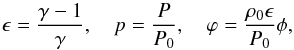
 (1)Measured velocity
dispersions are density-weighted projections of the three-dimensional velocity dispersions
along lines of sight through the cluster. Throughout the paper, we orient the coordinate
system such that the z-axis coincides with the line of sight. A projected
velocity dispersion profile is constructed by averaging over concentric cylinderical
shells drilled around the line of sight as a symmetry axis. This profile represents the
input of our method.
(1)Measured velocity
dispersions are density-weighted projections of the three-dimensional velocity dispersions
along lines of sight through the cluster. Throughout the paper, we orient the coordinate
system such that the z-axis coincides with the line of sight. A projected
velocity dispersion profile is constructed by averaging over concentric cylinderical
shells drilled around the line of sight as a symmetry axis. This profile represents the
input of our method.
The final output of our algorithm is the projected Newtonian potential of the lens,
defined by  (2)where
φ is the
three-dimensional gravitational potential of the cluster at distance Dd from the
observer. The projected potential is given as a function of the two-dimensional position
coordinate θ on the sky.
(2)where
φ is the
three-dimensional gravitational potential of the cluster at distance Dd from the
observer. The projected potential is given as a function of the two-dimensional position
coordinate θ on the sky.
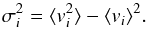
The geometry of the problem is sketched in Fig. 1 (see also Binney & Tremaine 1987). For simplicity during the construction of our method, we adopted a spherically-symmetric cluster model. All equations derived in the following are thus formulated in spherical coordinates.
 |
Fig. 1 Cluster geometry (see Binney & Tremaine 1987). |
The possible anisotropy of the velocity distribution is described by the conventional
anisotropy parameter β (Binney &
Tremaine 1987),  (3)Our algorithm
consists of three main steps:
(3)Our algorithm
consists of three main steps:
-
We deproject the observable, i.e. the velocity dispersions along the line of sight, into a deprojected quantity that, for reasons to be clarified later, is called the effective galaxy pressure P.
-
Since this effective pressure P is related to the DM gravitational potential φ, we can solve the Jeans equation using symmetry assumptions and a formal analogy to a polytropic gas stratification. We thus obtain a relation between the DM gravitational potential φ and the effective galaxy pressure. This equation is a Volterra integral equation of the second kind for φ, which can be solved iteratively.
-
Having obtained the gravitational potential, we simply project it to find the two-dimensional potential ψ.
We describe our deprojection method in Sect. 2.2.
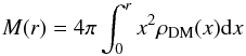
The relevant three-dimensional quantities are the galaxy density ρ, the dark matter density
ρDM, the mean radial velocity dispersion
 and the dark
matter gravitational potential φ. They are related via the Poisson and Jeans
equations. In spherical symmetry, the Poisson and Jeans equations are
and the dark
matter gravitational potential φ. They are related via the Poisson and Jeans
equations. In spherical symmetry, the Poisson and Jeans equations are 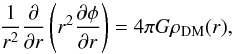 (4)and
 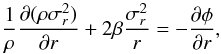 (5)respectively. We
note here that the second term on the left-hand side of Eq. (5) is the only formal difference to the hydrostatic equation for the
hot intracluster gas. This difference is important because it complicates the solution of
the Jeans equation considerably.
(5)respectively. We
note here that the second term on the left-hand side of Eq. (5) is the only formal difference to the hydrostatic equation for the
hot intracluster gas. This difference is important because it complicates the solution of
the Jeans equation considerably.
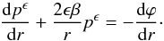
For solving the Jeans equation, we formally identify the density-weighted radial velocity
dispersion  with an effective
galaxy pressure P and assume that it is related to the density by a
polytropic relation. This assumption can be justified by the following calculation.
with an effective
galaxy pressure P and assume that it is related to the density by a
polytropic relation. This assumption can be justified by the following calculation.
A given radial density profile ρ(r) implies the mass profile
 (6)and, by
Poisson’s equation, the gravitational-potential gradient
(6)and, by
Poisson’s equation, the gravitational-potential gradient
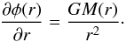 (7)With this
expression, the Jeans equation has the solution
(7)With this
expression, the Jeans equation has the solution 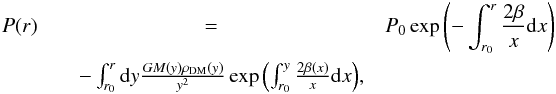 (8)where
the boundary conditions are set by the pressure P0 at the fiducial radius
r0. The fiducial pressure P0 can be
related to a fiducial density ρ0 via the virial theorem,
(8)where
the boundary conditions are set by the pressure P0 at the fiducial radius
r0. The fiducial pressure P0 can be
related to a fiducial density ρ0 via the virial theorem,
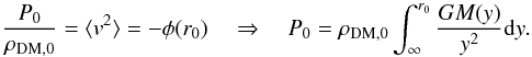 (9)This way, the effective
pressure profile of the cluster galaxies can be expressed in terms of the density and
anisotropy profiles. At this point, we devised a simple way to test our assumption in
which we restricted ourselves to a dissipationless case study. We evaluated Eq. (8) for two different mass density profiles, the
Hernquist (Hernquist 1990) and NFW (Navarro et al. 1996) profiles, adopting the anisotropy
profile derived by (Hansen & Moore 2006)
from detailed numerical studies. As Fig. 2 shows, the
effective pressure-density relation is nearly polytropic, i.e. an approximate power law.
Thus, our assumption of an effectively polytropic galaxy stratification,
(9)This way, the effective
pressure profile of the cluster galaxies can be expressed in terms of the density and
anisotropy profiles. At this point, we devised a simple way to test our assumption in
which we restricted ourselves to a dissipationless case study. We evaluated Eq. (8) for two different mass density profiles, the
Hernquist (Hernquist 1990) and NFW (Navarro et al. 1996) profiles, adopting the anisotropy
profile derived by (Hansen & Moore 2006)
from detailed numerical studies. As Fig. 2 shows, the
effective pressure-density relation is nearly polytropic, i.e. an approximate power law.
Thus, our assumption of an effectively polytropic galaxy stratification, 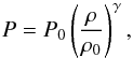 (10)seems
appropriate. In the numerical tests (see Sect. 3), we
do not make use of the Hansen & Moore
(2006) profile. We instead use the anisotropy profile directly obtained from the
data.
(10)seems
appropriate. In the numerical tests (see Sect. 3), we
do not make use of the Hansen & Moore
(2006) profile. We instead use the anisotropy profile directly obtained from the
data.
 |
Fig. 2 Relation (8) between the effective pressure and the density shown for the Hernquist and NFW density profiles and adopting the anisotropy parameter proposed by (Hansen & Moore 2006). The very nearly straight lines (note the logarithmic axes) demonstrate that the assumption of a polytropic relation is justified. |
With this result, we return to the Jeans Eq. (5), where we express the density by the effective pressure by means of Eq.
(10). For brevity, we further abbreviate
 (11)to cast the
Jeans equation (Eq. (5)) into the form
(11)to cast the
Jeans equation (Eq. (5)) into the form
 (12)This linear,
inhomogeneous, first-order differential equation with non-constant coefficients can be
solved straightforwardly, e.g. by variation of constants. The solution
(12)This linear,
inhomogeneous, first-order differential equation with non-constant coefficients can be
solved straightforwardly, e.g. by variation of constants. The solution 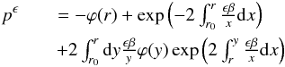 (13)is
the unique relation between the effective pressure and the gravitational potential we were
aiming at.
(13)is
the unique relation between the effective pressure and the gravitational potential we were
aiming at.
Equation (13) is a Volterra integral equation of second kind (Abramowitz & Stegun 1972) that can be solved iteratively. In this way, we find a relation between the effective pressure p and the gravitational potential ϕ. Projection along the line of sight leads to the two-dimensional potential ψ.
2.2. Deprojection
Observations yield the line of sight projection of only the galaxy velocity dispersion.
Different deprojection techniques by which it is possible to retrieve the
three-dimensional velocity dispersions are available. Each of these techniques has
strengths and weaknesses and the difficulty lies in choosing the optimal method according
to the situation one is considering. An option briefly discussed in Mamon & Boué (2010); Saha et
al. (1996) is the deprojection by Fourier transform. If proper integration
variables are chosen, projection can be considered as a convolution problem (see Eq.
(14)). A Fourier transform of this
convolution leads to a product in Fourier space which can be inverted easily. Transforming
back to real space yields the deprojected function1.
Another possibility is the Abel inversion used by Wolf et
al. (2010); Mamon & Boué (2010);
Biviano & Salucci (2006) and it
involves a differentiation of the data, which can be very problematic in presence of a low
signal-to-noise ratio. We adopted a third method, the Richardson-Lucy deconvolution (Richardson 1972; Lucy
1974; Binney & Mamon 1982). The
main weakness of this method is that it requires a normalisation of the data. In the case
we are studying, this was though the lowest disadvantage. A strength of this method is the
presence of a regularisation that helps control the noise. As detailed in Konrad et al. (2013), a line of sight-projection
g(s) is assumed to be related to a
three-dimensional quantity f(r) by 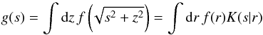 (14)with a projection kernel
K(s |
r). In spherical symmetry, with the anisotropy
parameter β(r), the projection kernel for the
velocity dispersion is
(14)with a projection kernel
K(s |
r). In spherical symmetry, with the anisotropy
parameter β(r), the projection kernel for the
velocity dispersion is 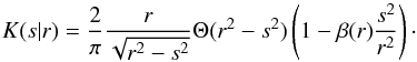 (15)For isotropic velocity
dispersions or an isotropic gas pressure, the final factor in parentheses in Eq. (15) is unity. The kernel in Eq. (15) can be easily derived from Fig. 1 as shown by Binney
& Tremaine (1987).
(15)For isotropic velocity
dispersions or an isotropic gas pressure, the final factor in parentheses in Eq. (15) is unity. The kernel in Eq. (15) can be easily derived from Fig. 1 as shown by Binney
& Tremaine (1987).
Provided that g(s), f(r) and
K(s |
r) are normalised2, the following iterative scheme follows from Bayes’ theorem (see Lucy 1974; Konrad et
al. 2013): 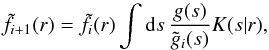 (16)where
 (17)Thus, starting from
a suitably guessed, normalised function
(17)Thus, starting from
a suitably guessed, normalised function  , the
scheme given by Eqs. (16) and (17) allows recovery of the three-dimensional
function f(r) from its two-dimensional
projection g(s), assuming the symmetry
incorporated into the projection kernel K(s | r).
Experience shows that even for guess functions that
are wildly different from the true f(r), the method converges
surprisingly quickly.
, the
scheme given by Eqs. (16) and (17) allows recovery of the three-dimensional
function f(r) from its two-dimensional
projection g(s), assuming the symmetry
incorporated into the projection kernel K(s | r).
Experience shows that even for guess functions that
are wildly different from the true f(r), the method converges
surprisingly quickly.
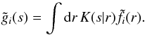
For applying this approach to realistic observational data containing small scale
fluctuations due to background or instrumental noise, a regularisation term should be
introduced as discussed in Lucy (1994). It was
shown there that the deprojection algorithm can be interpreted as the result of a
maximum-likelihood problem obtained by variation, ![Mathematical equation: \begin{equation} \label{var1} f_{i+1}(r) = f_i(r) + f_i(r)\left[ \frac{\delta H[f_i]}{\delta f_i(r)}- \int\d r\,f_i(r)\frac{\delta H[f_i]}{\delta f_i(r)} \right], \end{equation}](/articles/aa/full_html/2014/10/aa21748-13/aa21748-13-eq43.png) (18)where the functional
derivatives of the functional H [ f
]
(18)where the functional
derivatives of the functional H [ f
]![Mathematical equation: \begin{equation} H[f] = \int\d s\,g(s)\ln\tilde g(s) \end{equation}](/articles/aa/full_html/2014/10/aa21748-13/aa21748-13-eq45.png) (19)occur.
(19)occur.
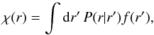
Regularisation can be introduced by adding a functional S [ f ],
![Mathematical equation: \begin{equation} H[f] \to Q[f] = H[f] + \alpha S[f], \label{eq:regularised_functional} \end{equation}](/articles/aa/full_html/2014/10/aa21748-13/aa21748-13-eq47.png) (20)which can have an
entropic form
(20)which can have an
entropic form ![Mathematical equation: \begin{equation} S[f] = -\int\d r\,f(r)\ln\frac{f(r)}{\chi(r)}\cdot \label{eq:24} \end{equation}](/articles/aa/full_html/2014/10/aa21748-13/aa21748-13-eq48.png) (21)Here,
χ(r) is a smooth prior function
chosen to suppress small scale fluctuations. A suitable prior can be the smoothed version
of the deprojection result from the previous iteration step. This choice, known as the
floating default (see Horne 1985; Lucy 1994), is defined by
(21)Here,
χ(r) is a smooth prior function
chosen to suppress small scale fluctuations. A suitable prior can be the smoothed version
of the deprojection result from the previous iteration step. This choice, known as the
floating default (see Horne 1985; Lucy 1994), is defined by
 (22)with a normalised,
usually sharply peaked convolution kernel P(r |
r′) symmetric in r −
r′. We use a properly normalised Gaussian
with a smoothing scale L,
(22)with a normalised,
usually sharply peaked convolution kernel P(r |
r′) symmetric in r −
r′. We use a properly normalised Gaussian
with a smoothing scale L,
 (23)Replacing the variation
of H [ f
] in Eq. (18) by the
variation of Q [
f ] from Eq. (20), we obtain
(23)Replacing the variation
of H [ f
] in Eq. (18) by the
variation of Q [
f ] from Eq. (20), we obtain ![Mathematical equation: \begin{eqnarray} \label{eq:iteration} f_{i+1}(r) &=& f_i(r)\left\{ \int\d s\,\frac{g(s)}{\tilde g_i(s)}K(s|r)\right.\\&\quad +\left. \alpha\left[1+S[f_i]+\ln\left(\frac{f_i(r)}{\chi_{i}(r)}\right)- \int\d r'\,\frac{f_i(r')}{\chi_{i}(r')}P(r|r')\right]\right\},\nonumber \end{eqnarray}](/articles/aa/full_html/2014/10/aa21748-13/aa21748-13-eq56.png) (24)which
we use henceforth. Since we are working with discretised data sets, the integrals in Eq.
(24) need to be approximated by sums.
(24)which
we use henceforth. Since we are working with discretised data sets, the integrals in Eq.
(24) need to be approximated by sums.
3. Numerical tests
We now proceed to demonstrate that it is possible to recover the projected gravitational potential ψ of a galaxy cluster from the measured velocity dispersions projected along the line of sight. The algorithm described in Sect. 2.1 assumes spherical symmetry and a polytropic relation between the effective galaxy pressure and the density.
Feeding the projected velocity dispersions into the Richardson-Lucy deprojection, we obtain the effective pressure P related to the gravitational potential φ by Eq. (13). Once this is achieved, the gravitational potential just needs to be projected along the line of sight. We perform the reconstruction for three distinct lines of sight, chosen to be parallel to the x-, y- and z-axes respectively.
3.1. The data
For testing our algorithm with simulated data, we require a velocity-dispersion profile projected along the line of sight and a two-dimensional gravitational potential obtained independently. We obtain such data from one of the clusters (denoted g1) in the hydrodynamically simulated sample described in (Saro et al. 2006) and used previously in (Meneghetti et al. 2010). The g1 cluster has a virial mass M200 = 1.14 × 10¹⁵ h-1M⊙ and is located at a redshift z = 0.297. We start from a catalogue listing the Cartesian coordinates and the three Cartesian velocity components of simulation particles tracking the motion of cluster galaxies. All information necessary for the kinematic analysis described in Sect. 3.2 can be extracted from this catalogue.
In addition, we converted the surface-mass density of the cluster into the two-dimensional potential, solving Poisson’s equation by means of a fast-Fourier transform. The surface-density map and the two-dimensional gravitational potential are shown in Fig. 3. Evidently, the potential is considerably smoother than the mass density.
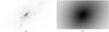 |
Fig. 3 a) Surface-mass density of the simulated cluster g1 in the x-y plane. b) Two-dimensional gravitational potential obtained from the surface-density map solving Poisson’s equation via fast-Fourier transform. Both images show regions with 10 h-1 Mpc side length. |
To enforce axial symmetry, we azimuthally average the gravitational potential shown in Fig. 3b around the centre, chosen to be the point with the deepest (most negative) potential. To make it comparable to the outcome of our algorithm, it can be passed into the RL deprojection (with β = 0) yielding the gravitational potential which can then be appropriately shifted and normalised.
3.2. Testing the algorithm
The assumption of spherical symmetry suggests spherical polar coordinates as a natural
choice for describing the system. After transforming the velocity components to this
coordinate frame, the number-density profile of the cluster galaxies is obtained within
radial bins ri centred on the
cluster centre chosen to contain equal numbers of galaxies. The number counts are then
converted to a number-density profile by weighting with the inverse volume of each radial
shell,  (25)Figure 5 reveals that the number-density profile for this
particular cluster essentially follows a power law. In a first approximation that is
sufficient for our purposes, galaxy biasing and variations of the galaxy mass function are
neglected, allowing us to adopt the number density as a direct tracer of the mass density.
(25)Figure 5 reveals that the number-density profile for this
particular cluster essentially follows a power law. In a first approximation that is
sufficient for our purposes, galaxy biasing and variations of the galaxy mass function are
neglected, allowing us to adopt the number density as a direct tracer of the mass density.
Given the number-density profile and the radial bins, a mean galaxy velocity can be
obtained in each radial shell. The variance of the velocities about this mean yields the
galaxy velocity-dispersion profiles ,
 and
and
 in the
radial, azimuthal and polar directions. These quantities enable us to derive the profile
of the anisotropy parameter according to the definition in Eq. (3). The result is shown in Fig. 4, where we fit the two-parameter model
in the
radial, azimuthal and polar directions. These quantities enable us to derive the profile
of the anisotropy parameter according to the definition in Eq. (3). The result is shown in Fig. 4, where we fit the two-parameter model
 (26)proposed
by Mamon & Łokas (2005), generalised by
Tiret et al. (2007) and used in Mamon et al. (2013). This fitted profile is the best
option available in the literature but the substantial scatter (also noted by Wojtak et al. 2008; Mamon et al. 2013) convinced us to use the profile-averaged mean value of
β. We have
also considered a linear interpolation of the data points, but this leads to unconvincing
results for the gravitational potential, because the scatter in the interpolated
anisotropy profile strongly affects the results of the Volterra equation.
(26)proposed
by Mamon & Łokas (2005), generalised by
Tiret et al. (2007) and used in Mamon et al. (2013). This fitted profile is the best
option available in the literature but the substantial scatter (also noted by Wojtak et al. 2008; Mamon et al. 2013) convinced us to use the profile-averaged mean value of
β. We have
also considered a linear interpolation of the data points, but this leads to unconvincing
results for the gravitational potential, because the scatter in the interpolated
anisotropy profile strongly affects the results of the Volterra equation.
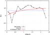 |
Fig. 4 Radial profile of the anisotropy parameter β(r) defined in Eq. (3), obtained from the simulated cluster data. The two-parameter model by (Mamon & Łokas 2005) is fitted to the data points. We find β∞ = 0.66 ± 0.36 and rβ = 0.82 ± 1.11. Concerning this result, a vanishing β would also be allowed. |
We weigh the radial velocity dispersions with the
number density and obtain the effective galaxy pressure. Projecting this quantity along
the line of sight,  (27)with the projection
kernel K(s |
r) defined in Eq. (15), we finally complete the input for our method which would be a
proper observable provided by observations. The observed velocity dispersions are
quantities projected along the line of sight and are thus implicitly weighted by the
number density of galaxies along the line of sight.
(27)with the projection
kernel K(s |
r) defined in Eq. (15), we finally complete the input for our method which would be a
proper observable provided by observations. The observed velocity dispersions are
quantities projected along the line of sight and are thus implicitly weighted by the
number density of galaxies along the line of sight.
Figure 6 is a double-logarithmic plot of the
effective galaxy pressure vs. the density, confirming that our polytropic assumption is
reasonable. The mean polytropic index γ, introduced in Sect. 2.1, is estimated from it by linear regression. Assuming that the
effective pressure is almost polytropic and that the mean polytropic index is close to
unity (our estimated value is γ = 0.915 ± 0.022) has an interesting implication
for the functional form of the distribution function. Owing to the spherically symmetric
geometry of our system, we can expect that it will be independent of the angular momentum
and of the form:  (28)where
 is the
relative energy. Such a distribution function allows Poisson equation to be rewritten in
the form of Lane-Emden equation (Binney & Tremaine
1987):
is the
relative energy. Such a distribution function allows Poisson equation to be rewritten in
the form of Lane-Emden equation (Binney & Tremaine
1987):  (29)In
the case of polytropic gases, it is possible to show that
(29)In
the case of polytropic gases, it is possible to show that
 .
A look at Fig. 6 suggests that in the case we are
considering γ ≈
0.9, which corresponds to a value of n ≈ −10 and to a
distribution function that goes like f(ℰ) ∝ ℰ-11.5. The distribution function
is thus a very steep function of the relative energy, which implies that the distribution
of the velocities of the cluster galaxies is nearly Maxwellian. This behaviour is exactly
what we expect in the case of a gaseous polytrope with adiabatic index γ ≃ 1.
.
A look at Fig. 6 suggests that in the case we are
considering γ ≈
0.9, which corresponds to a value of n ≈ −10 and to a
distribution function that goes like f(ℰ) ∝ ℰ-11.5. The distribution function
is thus a very steep function of the relative energy, which implies that the distribution
of the velocities of the cluster galaxies is nearly Maxwellian. This behaviour is exactly
what we expect in the case of a gaseous polytrope with adiabatic index γ ≃ 1.
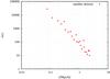 |
Fig. 5 Number density profile of the simulated cluster galaxies vs. the radius. It is obtained by galaxy number counts in spherical shells. |
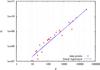 |
Fig. 6 Effective galaxy pressure vs. the density. The relation is represented by a power law, supporting our assumption of an effective polytropic relation. The mean polytropic index, as derived by linear regression, is γ = 0.915 ± 0.022. |
Figure 7 illustrates our complete algorithm. In the top left-hand panel, we show the normalised, line of sight projected velocity dispersions as a function of the projected radius and weighted with the galaxy number density. In the top right-hand panel, the normalised effective pressure profile obtained from the Richardson-Lucy deprojection algorithm is displayed. We then invert Eq. (13) to obtain the three-dimensional, Newtonian gravitational potential shown in the bottom left-hand panel. In the bottom right-hand panel, we finally show the derived two-dimensional gravitational potential.
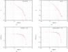 |
Fig. 7 Results of the four different steps comprising our algorithm. a) The input to our pipeline is the normalised, line of sight projected velocity-dispersion profile as a function of the projected radius and weighted by the galaxy number density. b) The Richardson-Lucy deprojection algorithm yields an effective galaxy-pressure profile. c) Solving the Volterra integral equation (Eq. (13)), we obtain the three-dimensional, Newtonian potential. d) The last step consists in projecting the gravitational potential of panel c) to find the two-dimensional potential. |
Figure 7 provides an overview of the first test we performed on our algorithm and shows all steps needed to reconstruct the two-dimensional potential from the line of sight projected velocity dispersions. A comparison between our reconstructed profiles and the true three- and two-dimensional gravitational potentials is now in order. We define as “true” the potentials extracted directly from the numerically simulated cluster.
Figure 8a shows the comparison between the
reconstructed and the true gravitational potentials, while Fig. 8b compares the reconstructed and the true projected potentials. The
reconstruction was performed three times with the line of sight axis chosen to be in turn
the x-, the
y- and the
z-axis. For
better visibility, the additional point sets are multiplied by factors of 0.5 for the y-axis case and
0.3 for the z-axis case. For easier
comparison of both potentials, their zero points and normalisations are adjusted3. To be consistent with Konrad et al. (2013), we decided to normalise both functions to unity and fix
φ(rmax) = 0. In Fig.
9, the relative deviation
 (30)between the reconstructed
and the true two-dimensional potentials is shown as a function of projected radius. The
deviation strongly increases at large radii, although it remains below 10% within 1.5 h-1 Mpc, which is similar to
the virial radius of the cluster.
(30)between the reconstructed
and the true two-dimensional potentials is shown as a function of projected radius. The
deviation strongly increases at large radii, although it remains below 10% within 1.5 h-1 Mpc, which is similar to
the virial radius of the cluster.
3.3. Application to observed data
The numerical tests presented above were run on line-of-sight projected data extracted from a simulated galaxy cluster. Starting from spatial Cartesian coordinates and velocity components of a sample of member galaxies, the effective galaxy pressure was obtained by weighting the squared radial velocity dispersion with the number density. Afterwards, the required observable was constructed by projection along the line of sight. The effective polytropic index γ and the profile β(r) of the anisotropy parameter could be easily obtained from the simulated sample. Unfortunately, neither of the last two quantities is directly accessible to observations. Therefore a method needs to be proposed that allows modelling the effective polytropic index and the anisotropy profile.
Major efforts have been undertaken in recent years to either constrain the anisotropy profile from observational and simulated data (Lemze et al. 2009; Mamon et al. 2013) or to identify a general relation describing it (Mamon & Łokas 2005; Hansen & Moore 2006). The main objective of our work is to reconstruct the projected gravitational potential of a galaxy cluster. However, we can envisage an inverse application of our algorithm. By an operation analogous to Lemze et al. (2009), it is possible to constrain β(r) using simultaneously information from gravitational lensing and galaxy kinematics. The existence of multiple constraints on the two-dimensional potential ψ also allows developing an iterative method for constraining β(r) and γ.
Within the CLASH survey project, considerable progress has been made in reproducing the observed CLASH clusters by simulations (Meneghetti et al., in prep.). These results would possibly enable us to guess a polytropic index and an anisotropy profile that could then be combined with kinematic data from observations in order to improve our reconstruction.
4. Conclusions
With the study presented here, we have continued our series of papers aiming at parameter-free reconstructions of the projected gravitational potential of galaxy clusters. The essential goal of our approach is thus to construct methods to relate all cluster observables to the two-dimensional gravitational potential. In a previous paper, we showed how this can be achieved with one of the two cluster observables based on the hot intracluster gas, i.e. X-ray emission, and we plan to extend our method to the thermal Sunyaev-Zel’dovich effect in the future. In this paper, we address the problem of how the observed line-of-sight projected velocity dispersions of cluster galaxies can be converted to the projected gravitational potential. We propose a solution that closely follows our interpretation of the observables provided by the intracluster plasma, but necessarily differs from it in the crucial aspect that the velocity dispersion of the cluster galaxies, unlike the gas pressure, can be anisotropic.
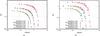 |
Fig. 8 Reconstructed gravitational potentials in a) three and b) two dimensions are plotted as functions of radius and compared with the true potentials. In each panel, the blue, light blue and sky blue points show the true potential determined from the convergence map, while the red, orange and yellow points show the result of our reconstruction method. The corresponding relative deviation as a function of radius assuming the z-axis as a line of sight is shown in Fig. 9. |
The algorithm we proposed rests on the following crucial assumptions. First, we assumed that the effective galaxy pressure, by which we mean the product of the galaxy number density and the radial velocity dispersion, can be related to the density itself by a polytropic relation, i.e. a power law. We tested this assumption with different density profiles and functional forms of the anisotropy parameter and found it to be satisfied. Second, by adopting this polytropic relation, we solved the radial component of the Jeans equation, relating the effective galaxy pressure to the dark matter potential gradient. This solution can be analytically given in the form of a Volterra integral equation of second kind for the three-dimensional gravitational potential, which can be solved by iteration. Thus, we established a relation between the three-dimensional gravitational potential and the effective galaxy pressure.
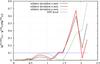 |
Fig. 9 The relative deviation between the reconstructed and true two-dimensional gravitational potentials where the line of sight is taken along the z-axis is shown here as a function of distance from the cluster center. The deviation remains moderate (below 10 %) within a radius of approximately 1.5 h-1 Mpc. |
The effective galaxy pressure itself can be obtained from the observable, line of sight projected galaxy velocity dispersions by Richardson-Lucy deprojection. The two-dimensional gravitational potential can finally be found by straightforward projection along the line of sight.
We have tested this algorithm on a simulated galaxy cluster in which galaxies have been identified. This cluster is part of a sample of numerical hydrodynamical simulations described in Saro et al. (2006) and used in Meneghetti et al. (2010). The anisotropy profile β(r), as well as the mean effective polytropic index γ, were obtained directly from the simulation. Although these quantities can hardly be directly measured from observations, and it has up to now been impossible to give general prescriptions of their behaviour, it may well be justified to calibrate them on numerical simulations without introducing an unacceptable bias.
The numerical simulation shows that the anisotropy profile shown in Fig. 4 may be poorly constrained by the given simulation. The fit performed by the model suggested by Mamon & Łokas (2005) covers a wide range of possible behaviour. Reconstructing the two-dimensional potential based on the nominal mean value of the anisotropy profile yields a result that closely follows the numerical expectation out to ≈1.5 h-1 Mpc, as demonstrated by the relative deviation of the reconstructed from the true projected gravitational potential (see Fig. 9). The deviation remains below 10% in this radial range. Figure 6 confirms the approximate treatment of our system as a polytropic stratification.
The main limitation of our algorithm so far lies in the assumption of spherical symmetry, which we plan to relax by extending our method to the axially (rather than spherically) symmetric case.
We are planning to proceed by applying the algorithm devised here to observational data that could possibly be provided by the CLASH survey. In addition, we will focus on unifying the two algorithms presented in Konrad et al. (2013) and this paper so as to allow a single, joint reconstruction of the two-dimensional potential of galaxy clusters using lensing, X-ray and kinematic data.
A quantitative statement about the relative performance of the individual and joint methods we are proposing is intrinsically bound to the quality of the data sets that will be used to do the analysis. However, we can envisage at least three possible applications of the combination of potentials derived from them. First, especially in clusters at low redshift, the gravitational potential obtained from galaxy dynamics will extend to larger scales than the potential from gravitational lensing. In order to recover the radial profile of the matter distribution and to measure scale radii accurately, long lever arms are needed, and galaxy dynamics adds information from intermediate and large radii. Second, the dynamics of mass-less compared to the dynamics of massive particles tests the theory of gravity. Therefore, combinations of potentials reconstructed from lensing and from galaxy dynamics may be particularly important for this purpose if the individual potentials can be reconstructed accurately enough. Third, among the observables which cluster potentials can be recovered from, strong and weak lensing neither need mechanical nor hydrostatic nor thermal equilibrium, galaxy dynamics needs mechanical equilibrium, and the X-ray emission and the thermal SZ effect additionally needs hydrodynamical and thermal equilibrium. Comparing the results will directly allow testing these equilibrium conditions.
See Kalal & Nugent (1988) for a more detailed discussion.
The kernel K(s | r) is normalised integrating over s.
Note that due to the normalisation constraint of the Richardson-Lucy deprojection, we obtain a function proportional to φ. The potential extracted from the simulation has to be normalised in the same way. Since both potentials are obtained from different datasets providing different spatial boundaries, they need to be appropriately shifted (gauged) by adding a constant factor.
Acknowledgments
This work was supported in part by contract research “Internationale Spitzenforschung II-1” of the Baden-Württemberg Stiftung, by the Collaborative Research Centre TR 33 and project BA 1369/17 of the Deutsche Forschungsgemeinschaft. ES wishes to warmly thank Lauro Moscardini for his kind hospitality in Bologna and for the useful and insightful discussions and Gary Mamon for his helpful comments to this paper.
References
- Abramowitz, M., & Stegun, I. A. 1972, Handbook of Mathematical Functions (New York: Dover) [Google Scholar]
- Albrecht, A., Bernstein, G., Cahn, R., et al. 2006, submitted [arXiv:astro-ph/0609591] [Google Scholar]
- Bartelmann, M.,Narayan, R.,Seitz, S., &Schneider, P. 1996, ApJ, 464, L115 [NASA ADS] [CrossRef] [Google Scholar]
- Binney, J., &Mamon, G. A. 1982, MNRAS, 200, 361 [NASA ADS] [CrossRef] [Google Scholar]
- Binney, J., & Tremaine, S. 1987, Galactic dynamics (Porincetan University press) [Google Scholar]
- Biviano, A., &Salucci, P. 2006, A&A, 452, 75 [NASA ADS] [CrossRef] [EDP Sciences] [Google Scholar]
- Bradač, M., Schneider, P.,Lombardi, M., &Erben, T. 2005, A&A, 437, 39 [NASA ADS] [CrossRef] [EDP Sciences] [Google Scholar]
- Cacciato, M.,Bartelmann, M.,Meneghetti, M., &Moscardini, L. 2006, A&A, 458, 349 [NASA ADS] [CrossRef] [EDP Sciences] [Google Scholar]
- Coe, D.,Umetsu, K.,Zitrin, A., et al. 2012, ApJ, 757, 22 [NASA ADS] [CrossRef] [Google Scholar]
- Jde ong, J. T. A., Verdoes Kleijn, G. A.,Kuijken, K. H., &Valentijn, E. A. 2013, Exp. Astron., 35, 25 [Google Scholar]
- Hansen, S. H., &Moore, B. 2006, New Astron., 11, 333 [NASA ADS] [CrossRef] [Google Scholar]
- Hernquist, L. 1990, ApJ, 356, 359 [NASA ADS] [CrossRef] [Google Scholar]
- Horne, K. 1985, in Interacting Binaries, eds. P. P. Eggleton, & J. E. Pringle, NATO ASIC Proc., 150, 327 [Google Scholar]
- Kalal, M., &Nugent, K. A. 1988, Appl. Opt., 27, 1956 [NASA ADS] [CrossRef] [Google Scholar]
- Konrad, S.,Majer, C. L.,Meyer, S.,Sarli, E., &Bartelmann, M. 2013, A&A, 553, A118 [NASA ADS] [CrossRef] [EDP Sciences] [Google Scholar]
- Laureijs, R., Amiaux, J., Arduini, S., et al. 2011, submitted [arXiv:1110.3193] [Google Scholar]
- Lemze, D.,Broadhurst, T.,Rephaeli, Y.,Barkana, R., &Umetsu, K. 2009, ApJ, 701, 1336 [NASA ADS] [CrossRef] [Google Scholar]
- Lucy, L. B. 1974, AJ, 79, 745 [NASA ADS] [CrossRef] [Google Scholar]
- Lucy, L. B. 1994, A&A, 289, 983 [NASA ADS] [Google Scholar]
- Mamon, G. A., &Boué, G. 2010, MNRAS, 401, 2433 [NASA ADS] [CrossRef] [Google Scholar]
- Mamon, G. A., &Łokas, E. L. 2005, MNRAS, 363, 705 [NASA ADS] [CrossRef] [Google Scholar]
- Mamon, G. A.,Biviano, A., &Boué, G. 2013, MNRAS, 429, 3079 [NASA ADS] [CrossRef] [Google Scholar]
- Medezinski, E.,Umetsu, K.,Nonino, M., et al. 2013, ApJ, 777, 43 [NASA ADS] [CrossRef] [Google Scholar]
- Meneghetti, M.,Rasia, E.,Merten, J., et al. 2010, A&A, 514, A93 [NASA ADS] [CrossRef] [EDP Sciences] [Google Scholar]
- Merten, J.,Cacciato, M.,Meneghetti, M.,Mignone, C., &Bartelmann, M. 2009, A&A, 500, 681 [NASA ADS] [CrossRef] [EDP Sciences] [Google Scholar]
- Navarro, J. F.,Frenk, C. S., &White, S. D. M. 1996, ApJ, 462, 563 [NASA ADS] [CrossRef] [Google Scholar]
- Postman, M.,Coe, D.,Benítez, N., et al. 2012, ApJS, 199, 25 [NASA ADS] [CrossRef] [Google Scholar]
- Richardson, W. H. 1972, J. Opt. Soc. Am., 62, 55 [Google Scholar]
- Saha, P.,Bicknell, G. V., &McGregor, P. J. 1996, ApJ, 467, 636 [NASA ADS] [CrossRef] [Google Scholar]
- Saro, A.,Borgani, S.,Tornatore, L., et al. 2006, MNRAS, 373, 397 [NASA ADS] [CrossRef] [Google Scholar]
- Schneider, P. 2006, Extragalactic Astronomy and Cosmology: An Introduction, 1st edn. (Springer) [Google Scholar]
- Tiret, O.,Combes, F.,Angus, G. W.,Famaey, B., &Zhao, H. S. 2007, A&A, 476, L1 [NASA ADS] [CrossRef] [EDP Sciences] [Google Scholar]
- Wojtak, R.,Łokas, E. L.,Mamon, G. A., et al. 2008, MNRAS, 388, 815 [NASA ADS] [CrossRef] [Google Scholar]
- Wolf, J.,Martinez, G. D.,Bullock, J. S., et al. 2010, MNRAS, 406, 1220 [NASA ADS] [Google Scholar]
All Figures
|
Fig. 1 Cluster geometry (see Binney & Tremaine 1987). |
| In the text | |
|
Fig. 2 Relation (8) between the effective pressure and the density shown for the Hernquist and NFW density profiles and adopting the anisotropy parameter proposed by (Hansen & Moore 2006). The very nearly straight lines (note the logarithmic axes) demonstrate that the assumption of a polytropic relation is justified. |
| In the text | |
|
Fig. 3 a) Surface-mass density of the simulated cluster g1 in the x-y plane. b) Two-dimensional gravitational potential obtained from the surface-density map solving Poisson’s equation via fast-Fourier transform. Both images show regions with 10 h-1 Mpc side length. |
| In the text | |
|
Fig. 4 Radial profile of the anisotropy parameter β(r) defined in Eq. (3), obtained from the simulated cluster data. The two-parameter model by (Mamon & Łokas 2005) is fitted to the data points. We find β∞ = 0.66 ± 0.36 and rβ = 0.82 ± 1.11. Concerning this result, a vanishing β would also be allowed. |
| In the text | |
|
Fig. 5 Number density profile of the simulated cluster galaxies vs. the radius. It is obtained by galaxy number counts in spherical shells. |
| In the text | |
|
Fig. 6 Effective galaxy pressure vs. the density. The relation is represented by a power law, supporting our assumption of an effective polytropic relation. The mean polytropic index, as derived by linear regression, is γ = 0.915 ± 0.022. |
| In the text | |
|
Fig. 7 Results of the four different steps comprising our algorithm. a) The input to our pipeline is the normalised, line of sight projected velocity-dispersion profile as a function of the projected radius and weighted by the galaxy number density. b) The Richardson-Lucy deprojection algorithm yields an effective galaxy-pressure profile. c) Solving the Volterra integral equation (Eq. (13)), we obtain the three-dimensional, Newtonian potential. d) The last step consists in projecting the gravitational potential of panel c) to find the two-dimensional potential. |
| In the text | |
|
Fig. 8 Reconstructed gravitational potentials in a) three and b) two dimensions are plotted as functions of radius and compared with the true potentials. In each panel, the blue, light blue and sky blue points show the true potential determined from the convergence map, while the red, orange and yellow points show the result of our reconstruction method. The corresponding relative deviation as a function of radius assuming the z-axis as a line of sight is shown in Fig. 9. |
| In the text | |
|
Fig. 9 The relative deviation between the reconstructed and true two-dimensional gravitational potentials where the line of sight is taken along the z-axis is shown here as a function of distance from the cluster center. The deviation remains moderate (below 10 %) within a radius of approximately 1.5 h-1 Mpc. |
| In the text | |
Current usage metrics show cumulative count of Article Views (full-text article views including HTML views, PDF and ePub downloads, according to the available data) and Abstracts Views on Vision4Press platform.
Data correspond to usage on the plateform after 2015. The current usage metrics is available 48-96 hours after online publication and is updated daily on week days.
Initial download of the metrics may take a while.