| Issue |
A&A
Volume 569, September 2014
|
|
|---|---|---|
| Article Number | A15 | |
| Number of page(s) | 14 | |
| Section | Stellar structure and evolution | |
| DOI | https://doi.org/10.1051/0004-6361/201423611 | |
| Published online | 10 September 2014 | |
Asteroseismology revealing trapped modes in KIC 10553698A⋆,⋆⋆,⋆⋆⋆
1
Instituut voor Sterrenkunde, KU Leuven, Celestijnenlaan 200D,
3001
Leuven,
Belgium
e-mail:
This email address is being protected from spambots. You need JavaScript enabled to view it.
2
Nordic Optical Telescope, Rambla José Ana Fernández Pérez 7,
38711
Breña Baja,
Spain
3
Department of Physics, Astronomy, and Materials Science, Missouri
State University, Springfield, MO
65804,
USA
4
Uniwersytet Pedagogiczny w Krakowie, ul. Podchora¸żych 2,
30-084
Kraków,
Poland
5
Dr. Karl Remeis-Observatory & ECAP,
Astronomisches Inst., FAU
Erlangen-Nuremberg, 96049
Bamberg,
Germany
Received:
10
February
2014
Accepted:
10
June
2014
Abstract
The subdwarf-B pulsator, KIC 10553698A, is one of 16 such objects observed with a one-minute sampling rate for most of the duration of the Kepler mission. Like most of these stars, it displays a rich g-mode pulsation spectrum with several clear multiplets that maintain regular frequency splitting. We identify these pulsation modes as components of rotationally split multiplets in a star rotating with a period of ~41 d. From 162 clearly significant periodicities, we are able to identify 156 as likely components of ℓ = 1 or ℓ = 2 multiplets. For the first time we are able to detect ℓ = 1 modes that interpose in the asymptotic period sequences and that provide a clear indication of mode trapping in a stratified envelope, as predicted by theoretical models. A clear signal is also present in the Kepler photometry at 3.387 d. Spectroscopic observations reveal a radial-velocity amplitude of 64.8 km s-1. We find that the radial-velocity variations and the photometric signal have phase and amplitude that are perfectly consistent with a Doppler-beaming effect and conclude that the unseen companion, KIC 10553698B, must be a white dwarf most likely with a mass close to 0.6 M⊙.
Key words: subdwarfs / binaries: close / stars: oscillations / stars: individual: KIC 10553698
Based on observations obtained by the Kepler spacecraft, the Kitt Peak Mayall Telescope, the Nordic Optical Telescope, and the William Herschel Telescope.
Appendices A and B are available in electronic form at http://www.aanda.org
Tables A.1 and B.1 are also available in electronic form at the CDS via anonymous ftp to cdsarc.u-strasbg.fr (130.79.128.5) or via http://cdsarc.u-strasbg.fr/viz-bin/qcat?J/A+A/569/A15
© ESO, 2014
1. Introduction
Most hot subdwarf-B (sdB) stars belong to the population of extreme-horizontal-branch (EHB) stars. The HB designation implies that they have ignited helium through the core-helium flash, and therefore have a core mass close to the helium-flash mass of ~0.46 M⊙. But in order to reach B-star effective temperatures, they must have shed almost their entire hydrogen-rich envelope close to the tip of the red-giant branch. Several binary scenarios have been identified that can produce EHB stars, including either common-envelope ejection or stable Roche-lobe overflow (see Heber 2009, for a detailed review).
Like the main-sequence-B stars, the sdBs pulsate with short (p modes) and long periods (g modes) because of the iron-group elements opacity bump (κ mechanism), but at much shorter periods than their main-sequence counterparts. A key element in the driving of pulsations in these stars is the competition between radiative levitation and gravitational settling, which causes a local overabundance of iron in the driving zone (Charpinet et al. 1997; Fontaine et al. 2003). The hotter short-period pulsators are known as V361-Hya stars after the prototype (Kilkenny et al. 1997), and equivalently the cooler long-period pulsators are known as V1093-Her stars (Green et al. 2003), and they are collectively referred to as sdBV stars. Most stars are predominantly one or the other type, but a few stars in the middle of the temperature range are hybrids that show both types of pulsations in equal measure (Østensen 2009, and references therein).
The Kepler spacecraft spent four years monitoring a 105 deg2 field in the Cygnus-Lyrae region, with the primary goal of detecting transiting planets (Borucki et al. 2011). The high-quality lightcurves obtained by the spacecraft reveal a host of variable stars, providing a treasure trove for asteroseismic studies (Gilliland et al. 2010). In the first four quarters of the Kepler mission, a survey for pulsating stars was made, and a total of 113 compact-pulsator candidates were checked for variability by Østensen et al. (Østensen et al. 2010b; 2011 = Paper I). This very successful survey revealed one clear V361-Hya pulsator (Kawaler et al. 2010b) and one other transient short-period pulsator, and a total of thirteen V1093-Her stars (Reed et al. 2010; Kawaler et al. 2010a; Baran et al. 2011, Paper II), including an sdB+dM eclipsing binary in which the hot primary shows an exceptionally rich pulsation spectrum (Østensen et al. 2010a). Another three V1093-Her pulsators have been identified in the open cluster NGC 6791 (Pablo et al. 2011; Reed et al. 2012a), bringing the total number of sdBV stars in the Kepler field to eighteen. A closely related object was discovered in Kepler-archive data by Østensen et al. (2012); a BHB pulsator showing pulsation properties similar to the V1093-Her pulsators – the first such object discovered.
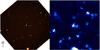 |
Fig. 1 Field images for KIC 10553698. The NOT/ALFOSC acquisition image (left) covers 2.5×2.5 arcmin, and the corresponding section from a Kepler full-frame image is also shown (right). The images are aligned so that north is up and east to the left. The target is the bright star in the centre of the field, and the four central pixels that are used for photometry for a typical quarter are outlined in the Kepler image. |
Since the series of early papers based on one-month datasets obtained during the survey phase of the Kepler mission, only seven of the g-mode pulsators have been subjected to detailed analysis based on many months of near-continuous data that the Kepler spacecraft gathered during the long-term monitoring phase. First, Charpinet et al. (2011a) analysed one year of data on KIC 5807616, revealing long-period periodicities that may be signatures of planets in very close orbit around the otherwise single sdB star. Baran (2012) analysed nine months of data on KIC 2697388, and Telting et al. (2012a) provided a detailed study of the 10-day sdBV+WD binary KIC 11558725, based on 15 months of data. The study of Baran & Winans (2012) analysed 27 months of data on KIC 2991403, KIC 2438324, and KIC 11179657. Most recently, Reed et al. (2014) have analysed the full 2.75 year dataset of KIC 10670103, providing mode identifications for 178 of 278 detected frequencies. While the papers by Van Grootel et al. (2010) and Charpinet et al. (2011b) matched asteroseismic models to observed frequencies based on survey data, no paper has yet attempted such forward modelling on a full two- to three-year Kepler dataset.
The target presented in this work, KIC 10553698, was included in the original survey and identified as a g-mode pulsator in Paper I. The one-month discovery run was examined in Paper II where 43 pulsation frequencies were identified. Thirty-seven of those frequencies were clearly in the g-mode region between 104 and 493 μHz, four were found in the intermediate region between 750 and 809 μHz, and two were in the high-frequency p-mode region at 3074 and 4070 μHz. Reed et al. (2011, Paper III) analysed the period spacing in this star along with thirteen other g-mode pulsators and made a first estimate of the mean period spacings for the non-radial g modes of degree ℓ = 1 and ℓ = 2.
Since those early Kepler papers, KIC 10553698 was monitored by Kepler throughout quarters 8 to 17, but skipping Q11 and Q15 when the object fell on CCD Module #3, which failed in January 2010. It is one of the brighter V1093-Hya stars in the sample, but it suffers some contamination in the Kepler photometry due to crowding from nearby stars, as illustrated in Fig. 1. Here we analyse all the available quarters of data from Q8 through to the end of the mission in Q17, and we provide a detailed frequency analysis with identification of the modes detected in the frequency spectrum. We also present new spectroscopic observations that demonstrate that KIC 10553698 is a single-lined spectroscopic binary with a 3.6 d orbital period. We refer to the pulsator as KIC 10553698A and the invisible companion as KIC 10553698B.
2. Spectroscopic observations
We observed KIC 10553698 as part of our observing campaign dedicated to investigating the binary status of the hot subdwarfs in the Kepler field (Telting et al. 2012b, 2014). From 2010 to 2012 we obtained 42 radial-velocity (RV) measurements of KIC 10553698, as listed in Table A.1. The first seven observations were made on each of six consecutive nights between August 25 and 30, 2010, using the ISIS long-slit spectrograph on the William Herschel Telescope (WHT), equipped with the R600B grating and using a 1.0′′ slit. It was already clear from this initial set of high signal-to-noise (S/N) observations that the target changes its RV with a peak-to-peak amplitude of ~130 km s-1 with a period of around three days.
Additional spectroscopy were collected with the ALFOSC spectrograph at the Nordic Optical Telescope (NOT) between May 2011 and October 2012. In total 24 spectra were collected over 18 nights using an 0.5′′ slit with grism #16. The final four of these were obtained using the spectrograph in vertical slit mode for fast readout. We found that these observations appear to be systematically shifted by ~30 km s-1 with respect to the other observations, indicating a problem with the wavelength calibration in this setup. These points were discarded rather than attempting to correct for the unexpected offset. A final set of ten spectra were obtained between September 29 and October 1, 2012, with the Kitt Peak 4-m Mayall telescope (KPNO) with RC-Spec/F3KB, the kpc-22b grating and a 2′′ slit. The WHT dataset is clearly the best with a S/N level close to 100 in each spectrum. The NOT data have variable quality between S/N ~ 20 and 80 depending on observing conditions, and the KPNO data have S/N ~ 50.
All spectra were processed and extracted using standard IRAF1 tasks. Radial velocities were computed with fxcor , by cross-correlating with a synthetic template derived from a fit to a mean spectrum of the target, and using the Hγ, Hδ, Hζ, and Hη lines. For the ALFOSC data, the final RVs were adjusted for the position of the target on the slit, judged from slit images taken just before and after the spectra. Table A.1 lists the observations with their mid-exposure dates, and RV measurements with the fxcor error (verr), as well as the observatory tabulated in the last column.
For the final determination of the RV amplitude we used the orbital period and phase as
determined from the Kepler photometry (see Sect. 3.1, below), since this can be determined much more accurately than from
the sparse spectroscopic observations. Fitting the amplitude and systemic velocity, we find
 The
phase-folded RV measurements are plotted together with the photometric orbital signal in
Fig. 4. The mass function is then
The
phase-folded RV measurements are plotted together with the photometric orbital signal in
Fig. 4. The mass function is then 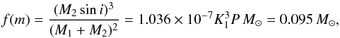 (1)which for a canonical
0.46 M⊙ primary, provides a minimum mass for the
secondary of 0.42 M⊙. Thus, unless the orbital inclination is
less than 29°,
KIC 10553698B must be a white dwarf (WD). For a
canonical 0.6 M⊙ WD, the inclination angle is
~52°.
(1)which for a canonical
0.46 M⊙ primary, provides a minimum mass for the
secondary of 0.42 M⊙. Thus, unless the orbital inclination is
less than 29°,
KIC 10553698B must be a white dwarf (WD). For a
canonical 0.6 M⊙ WD, the inclination angle is
~52°.
2.1. Atmospheric properties of the sdB
We determined Teff and log g from each of three mean spectra, co-added after correcting for the RV variation of the orbit. We redetermined the physical parameters of KIC 10553698A, using the H/He LTE grid of Heber et al. (2000) for consistency with Paper I. We used all the Balmer lines from Hβ to Hκ (excluding only the Hϵ line due to contamination with the Ca ii-H line) and the five strongest He i lines for the fit. The results are listed in Table 1, with the error-weighted mean in the bottom row. The errors listed on the measurements are the formal errors of the fit, which reflect the S/N of each mean, while the errors on the adopted values are the rms of the three measurements, which reflect the systematics of using different spectrographs more than the quality of the observations. These values and errors are relative to the LTE model grid and do not reflect any systematic effects caused by the assumptions underlying those models.
Physical parameters derived from the detrended mean spectra.
Fitted lines with equivalent widths larger then 50 mÅ.
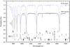 |
Fig. 2 Mean WHT spectrum of KIC 10553698 after correcting for the orbital velocity. The S/N in this mean spectrum peaks at ~200, and many weak metal lines can be distinguished in addition to the strong Balmer lines and He i lines at 4472 and 4026 Å. The continuum of the normalised spectrum was sampled individually in 100 Å sections. Shifted up by 0.2 is the model fit computed with tlusty/XTgrid. Line identifications are given for lines stronger than 30 mÅ in the model. The final parameters for this model fit are given in Table 3. |
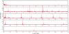 |
Fig. 3 FT of the full Kepler dataset of KIC 10553698. The ordinate axis has been truncated at 300 ppm to show sufficient details, even if there are some peaks in the FT that exceed this value. The 5σ level is indicated by a continuous line. |
We also fitted the mean WHT spectrum with the NLTE model atmosphere code tlusty (Hubeny & Lanz 1995). Spectral synthesis was done with synspec 49. Our models included H, He, C, N, O, Si and Fe opacities consistently in the calculations for atmospheric structure and synthetic spectra. The fit to the observation was done by the XTgrid fitting program (Németh et al. 2012). This procedure is a standard χ2-minimisation technique, which starts with a detailed model, and by successive approximations along the steepest gradient of the χ2, it converges on a solution. Instead of individual lines, the procedure fits the entire spectrum so as to account for line blanketing. However, the fit is still driven by the dominant Balmer lines with contributions from the strongest metal lines (listed in Table 2). The best fit was found with Teff = 27 750 K and log g = 5.45 dex, using the Stark broadening tables of Tremblay & Bergeron (2009). Errors and abundances for those elements that were found to be significant are listed in Table 3. When using the VCS Stark broadening tables for hydrogen (Lemke 1997), we found a systematically lower surface temperature and gravity, by 800 K and 0.06 dex. Parameter errors were determined by changing the model in one dimension until the critical χ2-value associated with the probability level at the given number of free parameters was reached. The resulting fit is shown together with the mean spectrum in Fig. 2. We used a resolution of Δλ = 1.7 Å and assumed a non-rotating sdB star.
Our NLTE model provides consistent parameters with the LTE analysis, indicating that NLTE effects are negligible in the atmosphere of KIC 10553698A. The abundances show that iron is supersolar, nitrogen is about half solar, whereas the other elements are significantly depleted with respect to their solar abundances. This pattern fits in the typical abundance pattern of sdB stars (see e.g. Geier 2013).
NLTE atmospheric parameters for the fit shown in Fig. 2, with respect to the solar abundances from Grevesse & Sauval (1998) provided for comparison.
3. Photometry and frequency analysis
KIC 10553698 has a magnitude in the Kepler photometric passband of Kp = 15.134 and colours g − r = −0.395 and g − i = −0.6942. It also appears in the 2mass catalogue as 2MASS J19530839+4743002 with J = 15.45(5), H = 15.54(9) but is below the detection limit in Ks. Its close proximity to several fainter stars makes the Kepler photometry suffer from contamination that varies slightly from quarter to quarter, depending on the positioning of the instrument’s 4′′-sized pixels. Figure 1 shows a 150′′-sized section of an ALFOSC target acquisition frame with the corresponding section of a Kepler full-frame image. For the frequency analysis, we used the optimally extracted lightcurves provided by the MAST3. These were detrended using low-order polynomials for each continuous lightcurve segment, removing only trends on month-long timescales. We experimented with using the pixel data in order to retain more flux from the target, but no significant improvement was achieved, so all the data presented here are based on the standard extraction provided by the archive pipeline.
3.1. The orbital signal
In the Fourier transform (FT) shown in Fig. 3, the
first significant peak is found at 3.41678 μHz, which corresponds to a period of 3.38743 d.
Since the span of the Kepler dataset is 855.6 d, the frequency resolution
is 0.014 μHz,
which coincidentally corresponds to a precision in period of 0.014 d. Thus, assuming a
circular orbit, we find an ephemeris for the system 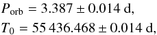 where
T0 is the time corresponding to zero phase
(where the subdwarf is at the closest point to the observer) for the first epoch of
observations. Since the orbital signal is too weak for single minima to be detected in the
point-to-point scatter, the uncertainty on the ephemeris phase is the same as that of the
Fourier analysis. Figure 4 shows the lightcurve
folded on this ephemeris and binned into 50 points. The error bars reflect the rms noise
in these bins, which may be boosted by the pulsation signal.
where
T0 is the time corresponding to zero phase
(where the subdwarf is at the closest point to the observer) for the first epoch of
observations. Since the orbital signal is too weak for single minima to be detected in the
point-to-point scatter, the uncertainty on the ephemeris phase is the same as that of the
Fourier analysis. Figure 4 shows the lightcurve
folded on this ephemeris and binned into 50 points. The error bars reflect the rms noise
in these bins, which may be boosted by the pulsation signal.
The photometric orbital signal seen in the Kepler lightcurve is caused
by the Doppler-beaming effect, as described in detail for the 0.4-d eclipsing sdB+WD
binary KPD 1946+4330 by Bloemen et al. (2011) and the 10-d sdBV+WD binary KIC 11558725 by Telting
et al. (2012a). KIC 10553698 is similar to the latter in that it only displays
the beaming signal and no ellipsoidal deformation, which would be present at
Porb/2, as is clearly seen in KPD 1946+4330 and also in KIC 6614501 (Silvotti et al. 2012).
For plain Doppler beaming, the observed flux from the target is related to the orbital
velocity along the line of sight, vr, as
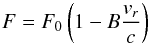 (2)where
F0 is the intrinsic flux of the star in
the observed passband, B the beaming factor, and vr/c the fraction of the
orbital velocity to the speed of light. The beaming factor has several terms, some
geometrical, and a part that depends on the spectrum of the radiating star. Since
KIC 10553698A has almost exactly the same
physical parameters as KIC 11558725, we simply
adopt the beaming factor computed by Telting et al.
(2012a), B = 1.403(5). Using the measured RV amplitude we can
then predict a beaming amplitude of BK1/c = 303 ± 10 ppm.
(2)where
F0 is the intrinsic flux of the star in
the observed passband, B the beaming factor, and vr/c the fraction of the
orbital velocity to the speed of light. The beaming factor has several terms, some
geometrical, and a part that depends on the spectrum of the radiating star. Since
KIC 10553698A has almost exactly the same
physical parameters as KIC 11558725, we simply
adopt the beaming factor computed by Telting et al.
(2012a), B = 1.403(5). Using the measured RV amplitude we can
then predict a beaming amplitude of BK1/c = 303 ± 10 ppm.
The observed beaming amplitude is 274 ± 6 ppm in the optimally extracted lightcurve, after applying minimal polynomial fits to remove long-term trends. Correcting for the crowding fraction indicated in the Kepler dataset, which states that the ratio of target flux to total flux is ~0.91 (see Table 4), the contamination-corrected beaming amplitude is 299 ppm, which is perfectly consistent with the predicted value.
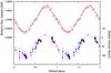 |
Fig. 4 Top: the 855.6 d Kepler lightcurve folded on the orbital period and binned into 50 bins. Bottom: radial velocity measurements folded on the same ephemeris as the lightcurve. (Red triangles: WHT; blue circles: NOT; black squares: KPNO.) |
Kepler pixel-data parameters.
3.2. The sliding FT
In Fig. 5 we show a sliding FT (sFT) of the same dataset as was used to generate Fig. 3. The data were chopped into segments of 12-d length and stepped with 4-d intervals, and the resulting FTs are stacked with time running in the y-direction to visualise the time variability of the modes. The black bands indicate the data gaps, most significantly the Q11 and Q15 gaps, when KIC 10553698 fell on the defunct Module #3. The thin black lines indicate the regular monthly data-downlink gaps of typically one-day duration, with slightly thicker lines indicating other events that caused interruptions to the observations for various reasons. A spacecraft artefact is seen close to f33 at ~370 μHz in Q8 and recurring every year, as described by Baran (2013).
It is easy to see from the sFT that some frequencies are single and very stable (e.g. f33, f69, and f123), and some produce stable beat patterns caused by doublets and triplets that are unresolved in the 12 d chunks (e.g. f79 − 81, f43−45, f36−37, and f63 − 64). At higher frequencies, f21−23, f24 − 26 and f28−31 form broader, more complex patterns that also appear to be completely stable throughout the duration of the observations. In the low-frequency range, the modes seem less stable, sometimes appearing or disappearing completely. For instance, the mode labelled f108−110 appears to have a similar beat period as that of the strongest mode, f79−81, but with an amplitude that increases throughout the run duration.
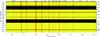 |
Fig. 5 Sliding FT for the region with the most significant pulsations in KIC 10553698. |
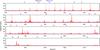 |
Fig. 6 Periodogram for KIC 10553698. This is the same FT as in Fig. 3, but with period on the abscissa. The first panel starts where the last panel in Fig. 3 ends, and frequencies shorter than the triplet at 86 μHz have been truncated. Radial order according to the asymptotic relation (Eq. (4)) is indicated on the top axis, with inward tick marks counting the ℓ = 1 spacing and outward tick marks counting the ℓ = 2 spacing. |
3.3. The Fourier spectrum
A careful analysis of the peaks in the FT of KIC 10553698 reveals 162 significant features. What can be considered significant is always a matter of interpretation in such analyses, especially when amplitude variability is present. Here we have only retained frequencies that appear well separated rather than try to include every peak that appears in a cluster, since many of them are likely to be caused by splittings produced by amplitude variability. We analysed both the FT of the full SC dataset, including all seven available quarters, as plotted in Fig. 5, and the FT of the two long runs from Q8–10 and Q12–14 separately. We set the detection limit to five times the mean level in the FT, σFT, which translates to 25.7 ppm for the 8-Q dataset and ~40 ppm for the 3-Q datasets. To be retained, we required every frequency to be above the respective 5σFT limit in at least one of these three sets.
The full list of frequencies is provided in Table B.1. The table lists the frequency, period, and amplitude of each detected mode, together with a tentative mode ID provided as a non-radial degree number ℓ and a radial order n, where one could be estimated based on the analysis of the échelle diagram discussed in Sect. 3.7, below. Also given is a “State” description indicating the stability of the mode. This is given as “stable”, “rising”, or “dropping” if the mode is present in both 3-Q datasets within ±0.05 μHz of the frequency detected in the 8-Q dataset, and “stable” to indicate that the amplitude does not change by more than 20% between the two 3-Q sets compared with the amplitude of the 8-Q set. Modes that are not detected in one of the 3-Q datasets are classified as “appearing” or “disappearing”, and modes that are only significant in the 8-Q dataset are labelled “noisy”. A few modes labelled “messy” are significant only in one of the 3-Q datasets, but because of cancellation effects, they make only a broad, non-significant peak in the 8-Q set.
3.4. Rotationally split triplets
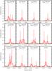 |
Fig. 7 Eleven highest amplitude frequencies in the KIC 10553698 Fourier spectrum. The bars indicate positions for the central m = 0 component (black), ℓ = 1, m = ±1 (blue), and ℓ = 2, m = ±1, 2 (magenta). |
In Fig. 7 we show the eleven strongest peaks together with the window function. It is quite clear from this figure already that many peaks appear in groups with a common spacing, as would be expected for rotationally split multiplets. The picture is not as clear as one may have wished. The strongest triplet, f79 − 81, shows slightly uneven splittings of δν = 0.168 and 0.155 μHz, respectively. The triplet f57−59 is perfectly even with a splitting of 0.159 μHz. Both are somewhat lopsided in amplitude, leaning either to the m = +1 or the m = –1 side. The three symmetric triplets f43 − 45, f52−54, and f36−37 have splittings of 0.132, 0.141, and 0.132 μHz, respectively.
The difference in rotational period that can be inferred from these splittings is quite significant (when using a simple model with a Ledoux constant, Cnℓ, of 0.5, as expected for high-order g-modes of degree ℓ = 1), ranging from 34.5 to 44.2 d. To indicate the rotational splitting in Figs. 7, 9, and B.1, we have used an average of the splittings measured in the three consecutive triplets identified as n = 11, 12, and 13, δν = 0.135 μHz, implying a rotational period of 42.9 d.
3.5. Quintuplets and the pulsation axis
Another spectacular sequence of multiplets can be found at higher frequencies. The four
peaks labelled f28 −
31 at 393 μHz form a perfectly even quintuplet with the
middle peak missing and a splitting of 0.235 μHz. The sequence f24−26 at
419 μHz
appears as three components of a quintuplet with splitting of 0.247 μHz, and f21−23
likewise matches three components of a quintuplet with splitting of 0.258 μHz. In all three cases
there are indications of the missing components close to the 5σFT limit. The
additional fact that this sequence of multiplets appears with a spacing of ~150 s = 260 s/ (see below) makes it very clear that this is a sequence of consecutive ℓ = 2 modes.
The rotational splitting for high-order g-modes in a uniformly rotating star is given by
Aerts et al.
(2010)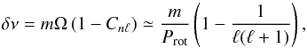 (3)so that the observed
splittings of the three consecutive ℓ = 2 multiplets translate to a rotation period of
41.0, 39.0, and 37.4 d, close to the middle of the range seen for the ℓ = 1 modes.
(3)so that the observed
splittings of the three consecutive ℓ = 2 multiplets translate to a rotation period of
41.0, 39.0, and 37.4 d, close to the middle of the range seen for the ℓ = 1 modes.
It is interesting that the middle m = 0 component is suppressed in this sequence of multiplets. This is very different from the quintuplet structure seen in KIC 10670103 (Reed et al. 2014) where the middle component is the strongest one. Geometric cancellation of ℓ,m = 2,0 occurs only when viewing a pulsator within a few degrees of i = 55°. At this angle there is no significant suppression of any particular ℓ = 1 component, consistent with what we have seen.
From the spectroscopic observations, we found that the mass function implies that the companion is consistent with a white dwarf for all orbital inclinations higher than 29°. If the pulsation axis is aligned with the orbital axis, the mass of the white dwarf must be close to 0.6 M⊙, which is the typical value for white dwarfs that are remnants of intermediate-mass stars after normal uninterrupted evolution.
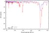 |
Fig. 8 KS test statistic for the full frequency list (red) and high-amplitude (A > 1000 ppm) modes (red) respectively. |
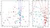 |
Fig. 9 Échelle diagram for ℓ = 1 (left) and ℓ = 2 (right). Detected modes are marked according to their period on the abscissa, with a cyclic folding on the asymptotic period on the ordinate axis. The right-hand axis gives the order n of the mode, according to the asymptotic relation (Eq. (4)). Blue circles mark modes identified as ℓ = 1, with outlined cyan circles indicating those that appear in multiplets. Red squares mark ℓ = 2 modes, again with outlined points indicating multiplets. Cyan diamonds mark trapped ℓ = 1 modes, red diamonds mark trapped ℓ = 2 modes, and green diamonds mark modes that do not fit either sequence. Outlined cyan squares indicate modes that can be either ℓ = 1 or ℓ = 2. The high-amplitude peaks (A > 250 ppm) in the full dataset are marked with enlarged symbols. |
3.6. The asymptotic period spacing
In the asymptotic limit of stellar pulsation theory, consecutive g modes follow the relation
 (4)where
L =
(4)where
L =  ,
Π0
is the reduced
period spacing in the asymptotic limit, and ϵℓ is a constant offset
for each ℓ.
,
Π0
is the reduced
period spacing in the asymptotic limit, and ϵℓ is a constant offset
for each ℓ.
A hallmark of the V1093 Her stars revealed by Kepler is that the
asymptotic period relation is readily detectable by the period spacings, ΔP of the modes (Reed et al. 2011, 2012b). The favoured method for determining the mean spacing is the
Kolmogorov-Smirnov (KS) test, which produces high negative values at the most frequently
observed spacing in a dataset. Figure 8 shows the KS
statistic for two period lists, the full set listed in Table B.1 and a list truncated to
contain only modes with amplitudes higher than 1000 ppm. A clear minimum is seen around
260 s in both sets. Only for the list including the low-amplitude modes does the KS test
show a second minimum at ΔP = 150 s. The
1/
relationship between these two peaks is the signature of the period difference between
ℓ = 1 and
ℓ = 2 modes
in the asymptotic approximation.
By plotting the P modulo ΔP versus P for the two period spacings, one can construct an échelle diagram for g-mode pulsators. Unlike the échelle diagram used for p-mode pulsators, which are evenly spaced in frequency and have the same spacing, Δν, for different orders ℓ, the g-mode échelle diagram must be folded on a different ΔP for each ℓ. Figure 9 shows the échelle diagrams for ℓ = 1 and ℓ = 2 for the 162 detected peaks in KIC 10553698A. After starting with the ΔP detected by the KS test, we made some iterations of identifying peaks and adjusting the spacing slightly until a reasonable picture emerged.
In the ℓ = 1 échelle diagram, one can clearly see a ridge of modes that meanders around the vertical lines drawn at ϵ = 180 s. The vertical lines curve to indicate how the frequency splitting for m = ±1 translate into period space. Two lines are drawn for each m to indicate the frequency resolution of the full dataset. The ℓ = 1 ridge includes almost all the most powerful modes, but a few are significantly off either sequence.
3.7. Assigning modes to observed periods
While some mode identifications are obvious based on multiplet structures, the deviations from a clear asymptotic sequence imply substantial ambiguities in the labelling. The identifications listed in Table B.1 should therefore not be taken as anything more than what the authors consider to be the most likely ones. Also, some frequencies listed are clearly spurious, caused by amplitude variability, since in several cases groups of four, or even five, peaks are listed as belonging to one ℓ = 1 triplet. In some cases the sequence for ℓ = 1 overlaps with the one of ℓ = 2, causing further ambiguity. For instance, in the case of f152−155 the two complex peaks (see Fig. B.1) are likely to be ℓ,n = 1, 35 and 2, 61, with the ℓ = 2 mode at ~107 μHz. Several other complex groups in Fig. B.1 are identified as superpositions of modes of different orders. In some cases, a particular group might be either ℓ = 1 or ℓ = 2, but has been identified based on the frequency splitting or because the identification for a given ℓ,n has already been assigned to a suitable mode.
While the majority of frequencies in Table B.1 can be identified in this scheme, some clearly fall well off either sequence. If these were all low-amplitude modes, we could dismiss them as ℓ = 3 or higher, but two of them appear among the highest amplitude peaks plotted in Fig. 7. The third strongest peak is the single and stable f123 at 140.5 μHz, which sits way out on the left edge in Fig. 9. It falls between the relatively low-amplitude multiplets assigned ID’s ℓ,n = 1, 26 and 1, 27, which both match the ℓ = 1 sequence well, and the nearest ℓ = 2 mode, n = 47, is also occupied. A similar problem appears with the pair f48−49, which is ranked as the 8th highest mode in amplitude. The pair appears with a splitting of 0.171 μHz, which is just slightly wider than that of the main f79−81 triplet. But it falls between two other higher-amplitude triplets assigned ℓ,n = 1, 12 and 1, 13. The spacing between those triplets is 302 s, so higher than the average period spacing, but much too tight to permit another ℓ = 1 mode to squeeze in. It is also sandwiched between two low-amplitude pairs assigned ℓ,n = 2, 22 and 2, 23. The remaining peaks that defy assignment in the asymptotic interpretation are all low amplitude and might well be ℓ > 2.
3.8. The trapped modes
The most plausible interpretation of the off-sequence, high-amplitude peaks is that they are trapped modes, which are produced mostly by the H/He transition in the stratified envelope as predicted by classical sdB models (Charpinet et al. 2000). To visualise the trapping signature, theoretical papers often show a period-spacing diagram where the period difference between consecutive modes are plotted against period. When reduced period, Π = PL, is used, modes with the same radial order, k, should overlap in this diagram. But to compute the required period differences, ΔΠ = Πk – Πk−1, we must have completely uninterrupted sequences. Note that when mode trapping occurs, extra modes are inserted into the asymptotic sequence, so that the real number of radial nodes in the star, k, is higher than the asymptotic order n.
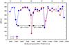 |
Fig. 10 Period difference between consecutive modes of the ℓ = 1 and ℓ = 2 sequences, after converting to reduced periods. The asymptotic order of the modes, n, is indicated on the upper axis. |
Inspecting the sequences of ℓ = 1 and ℓ = 2 modes listed in Table B.1, including the trapped modes that are marked as n = t in the table, we see that just a few modes are missing. To make a period-spacing diagram with an uninterrupted sequence of consecutive modes, we must check each case and see if we can find a suitable number to use in the sequence. Note that due to the huge number of independent frequencies in the full FT of the whole Kepler dataset, we have maintained a 5-σ significance threshold in order to avoid too many spurious frequencies. However, when looking at a specific frequency region suspected of containing a real frequency, it is justified to consider a 4-σ signal to be a significant detection.
The six modes needed to complete the sequences are ℓ = 1, n = 31, 32, ℓ = 2, n = 19, 32, 33, and an ℓ = 2 mode corresponding to the trapped ℓ = 1 mode between n = 26 and 27. For ℓ = 1, n = 31 there is a feature at the 4-σ level that we can use to complete the sequence of modes needed to construct the reduced period diagram. The same is the case for ℓ = 2, n = 19 and 33. The ℓ = 1, n = 32 mode should be at the position where the oddly spaced ℓ = 2 multiplet f143−146 is found, so we use the highest of these peaks to complete the sequence. A similar case can be made for ℓ = 2, n = 32, which should occur just where the highest peak in the FT is found, at ~202 μHz. And an ℓ = 2 mode to correspond with the trapped ℓ = 1 mode at Π = 10064 s would be located at 4109 s, which is in the region where another strong ℓ = 1 mode, f63, is seen.
After discovering the presence of trapped modes in KIC 10553698A, we revisited the table of frequencies to see if we could find evidence of other less obvious trapped modes. The only feature we could find that seems reasonable to interpret as a trapped mode is located between n = 19 and 20. The two modes f38 − 39 consist of a relatively high-amplitude stable peak with a noisy companion (shown in the first panel of Fig. B.1). It was first interpreted as ℓ = 1, but there are no missing ℓ = 1 modes in this region. As a trapped mode, it could be either ℓ = 1 or ℓ = 2. An ℓ = 1 interpetation would require a corresponding ℓ = 2 mode at ~1804 s, but this region is clean. An ℓ = 2 interpretation requires the corresponding ℓ = 1 mode to have an observed period of ~5412 s, at which we already find f90. This mode was first interpreted as the fourth component of an incomplete ℓ = 2 mode, even though the splitting did not match the expected one very well. Identifying f90 as the trapped ℓ = 1 mode corresponding to a trapped ℓ = 2 mode provides a closer match than it did as part of an ℓ = 2 multiplet. We therefore adopt this latter interpretation, but note that the identification for this trapped mode is not as clear as for the other two.
After completing the sequences by filling in for the six missing modes and the additional trapping feature between n = 19 and 20, the reduced-period diagram shown in Fig. 10 emerges. The modes identified in Table B.1 are marked with filled symbols and the missing modes with open symbols in the figure. All the observed multiplets have been reduced to a single period for this figure. For the triplets and the three clear ℓ = 2 multiplets we have inferred the position of the central component. For other modes, the case is much more ambiguous. In general, unless the period spacing could be interpreted in such a way as to locate the correct centre, we simply used the highest peak. At low n the error this produces is tiny, but at high n the error can be quite large. The curves plotted in the échelle diagrams and labelled on the top axis with the respective m, reflects this effect. The offset between the ℓ = 1 and 2 sequences in Fig. 10 increases at high n, which is most likely caused by such mode ambiguity rather than any physical effects.
The expected correspondence between the ℓ = 1 and ℓ = 2 sequences is striking. The diagram reveals three clear trapping features, where at least one is clearly present in both the ℓ = 1 and ℓ = 2 sequences. The first is at low radial order where the ℓ = 2 sequence is not present, and the last includes a “missing” ℓ = 2 point. The difference in reduced period between consecutive trapped modes can be seen to be ΠH = ~2400 and ~2730 s as indicated by the horizontal arrows in Fig. 10.
This observational reduced period diagram bears a striking resemblance to similar diagrams produced from theoretical models, e.g. Fig. 3 in Charpinet et al. (2002). The properties of this trapping structure depends on the mass of the H-rich envelope and the position of the transition zones inside the star (Charpinet et al. 2000). Both the transition zone between the hydrogen and helium layers in the envelope and the transition between the helium layer and the convective core, which with time develops an increasing carbon-oxygen content and thus a higher density, produce mode-trapping features that will affect the periods of the trapped modes (Charpinet et al. 2013). Due to the complexities of these double trapping zones it may not be straightforward to translate trapping period differences into asteroseismic ages on the EHB.
4. Conclusions
We have analysed the complete Kepler short-cadence lightcurve for KIC 10553698, and collected and analysed spectroscopic observations that reveal it to be a system consisting of a V1093-Her pulsator orbiting a white dwarf. When starting the frequency analysis of the pulsator, it soon became evident that a large number of the observed periodicities fitted neatly on the asymptotic sequences for ℓ = 1 and ℓ = 2, which is similar to what we have seen with the other V1093-Her pulsators in the Kepler field. However, when we realised that a few of the main modes were clearly incompatible with the asymptotic relation, we were immediately intrigued. By accepting two high-amplitude modes as trapped ℓ = 1 modes, we were finally able to make a convincing case that mode trapping, as predicted by all theoretical models for V1093-Her pulsators, is present and detectable in the Kepler observations. Thanks to almost perfectly complete sequences of consecutive ℓ = 1 and ℓ = 2 modes, we were able to, for the first time, generate an observed period-spacing diagram that shows convincing evidence for mode trapping. It is somewhat surprising that such features have not been spotted in other V1093-Her pulsators observed with Kepler. But it was only the high amplitude of two of the trapped modes, and the fact that all available ℓ = 1 modes in the sequence were already assigned, that tipped us off to this feature. For other pulsators, trapped modes may hide in the unassigned low-amplitude modes. It might be worthwhile revisiting the full sample of V1093-Her stars in light of this revelation.
Many ℓ = 1 and ℓ = 2 modes appear as rotationally split multiplets indicating rotational periods that range from 34.5 to 44.2 days, with the most convincing ℓ = 1 modes averaging to ~43 d and the best ℓ = 2 modes ~39 d. An accurate determination of the rotation rate from the observed multiplet splittings would require knowledge of the Cnℓ values from asteroseismic models. Until this becomes available we must be satisfied with the rough estimate Prot = 41±3 d. We also found that a series of clear ℓ = 2 multiplets all had the middle m = 0 component suppressed, implying a pulsation axis observed at close to 55°, which is the same value as would be required for the mass function of the binary to be compatible with a canonical sdB mass and a normal 0.6 M⊙white-dwarf. Since KIC 10553698B must have been the original primary of the progenitor system, the orbit must have been rather wide in order to allow it to complete its red-giant-branch evolution, followed by an asymptotic-giant-branch stage that brought it into contact with the main-sequence progenitor of the current primary, KIC 10553698A. The parameters of the KIC 10553698 system and others like it can be used to constrain the possible binary-interaction scenarios that allow enough angular momentum to be lost from the system to result in the observed configuration.
Online material
Appendix A: Radial velocity data
Radial velocity data.
Appendix B: Frequency data and figures
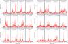 |
Fig. B.1 Some of the most significant peaks in the KIC 10553698A Fourier spectrum, following from the sequence shown in Fig. 7. |
Frequencies, periods, and amplitudes for KIC 10553698.
IRAF is distributed by the National Optical Astronomy Observatory; see http://iraf.noao.edu/
The Kepler Input Catalog does not provide errors on the magnitudes.
The Mikulski Archive for Space Telescopes is hosted by the Space Telescope Science Institute (STScI) at http://archive.stsci.edu/
Acknowledgments
The authors gratefully acknowledge the Kepler team and everybody who has
contributed to making this mission possible. Funding for the Kepler mission
is provided by the NASA Science Mission Directorate. We also thank Prof. Uli Heber for
kindly providing the model grids used for the LTE atmospheric analysis.The research leading
to these results has received funding from the European Research Council under the European
Community’s Seventh Framework Programme (FP7/2007–2013)/ERC grant agreement
N 227224
(prosperity), and from the Research Council of KU Leuven grant agreement
GOA/2008/04. Funding for this research was also provided by the US National Science
Foundation grants #1009436 and #1312869, and the Polish National Science Centre under
project N UMO-2011/03/D/ST9/01914.
The spectroscopic observations used in this work were collected at the Nordic Optical
Telescope (NOT) at the Observatorio del Roque de los Muchachos (ORM) on La Palma, operated
jointly by Denmark, Finland, Iceland, Norway, and Sweden; the William Herschel
Telescope (WHT) also at the ORM and operated by the Isaac Newton Group; and the
Mayall Telescope of Kitt Peak National Observatory, which is operated by the Association of
Universities for Research in Astronomy under cooperative agreement with the NSF.
227224
(prosperity), and from the Research Council of KU Leuven grant agreement
GOA/2008/04. Funding for this research was also provided by the US National Science
Foundation grants #1009436 and #1312869, and the Polish National Science Centre under
project N UMO-2011/03/D/ST9/01914.
The spectroscopic observations used in this work were collected at the Nordic Optical
Telescope (NOT) at the Observatorio del Roque de los Muchachos (ORM) on La Palma, operated
jointly by Denmark, Finland, Iceland, Norway, and Sweden; the William Herschel
Telescope (WHT) also at the ORM and operated by the Isaac Newton Group; and the
Mayall Telescope of Kitt Peak National Observatory, which is operated by the Association of
Universities for Research in Astronomy under cooperative agreement with the NSF.
References
- Aerts, C., Christensen-Dalsgaard, J., & Kurtz, D. W. 2010, Asteroseismology (Springer) [Google Scholar]
- Baran, A. S. 2012, Acta Astron., 62, 179 [NASA ADS] [Google Scholar]
- Baran, A. S. 2013, Acta Astron., 63, 203 [NASA ADS] [Google Scholar]
- Baran, A. S., & Winans, A. 2012, Acta Astron., 62, 343 [NASA ADS] [Google Scholar]
- Baran, A. S., Kawaler, S. D., Reed, M. D., et al. 2011, MNRAS, 414, 2871 [NASA ADS] [CrossRef] [Google Scholar]
- Bloemen, S., Marsh, T. R., Østensen, R. H., et al. 2011, MNRAS, 410, 1787 [NASA ADS] [Google Scholar]
- Borucki, W. J., Koch, D. G., Basri, G., et al. 2011, ApJ, 736, 19 [NASA ADS] [CrossRef] [Google Scholar]
- Charpinet, S., Fontaine, G., Brassard, P., et al. 1997, ApJ, 483, L123 [NASA ADS] [CrossRef] [PubMed] [Google Scholar]
- Charpinet, S., Fontaine, G., Brassard, P., & Dorman, B. 2000, ApJS, 131, 223 [Google Scholar]
- Charpinet, S., Fontaine, G., Brassard, P., & Dorman, B. 2002, ApJS, 139, 487 [Google Scholar]
- Charpinet, S., Fontaine, G., Brassard, P., et al. 2011a, Nature, 480, 496 [NASA ADS] [CrossRef] [PubMed] [Google Scholar]
- Charpinet, S., Van Grootel, V., Fontaine, G., et al. 2011b, A&A, 530, A3 [NASA ADS] [CrossRef] [EDP Sciences] [Google Scholar]
- Charpinet, S., Van Grootel, V., Brassard, P., et al. 2013, in Ageing Low Mass Stars: From Red Giants to White Dwarfs, EPJ Web Conf., 43, 4005 [Google Scholar]
- Fontaine, G., Brassard, P., Charpinet, S., et al. 2003, ApJ, 597, 518 [Google Scholar]
- Geier, S. 2013, A&A, 549, A110 [NASA ADS] [CrossRef] [EDP Sciences] [Google Scholar]
- Gilliland, R. L., Brown, T. M., Christensen-Dalsgaard, J., et al. 2010, PASP, 122, 131 [NASA ADS] [CrossRef] [Google Scholar]
- Green, E. M., Fontaine, G., Reed, M. D., et al. 2003, ApJ, 583, L31 [NASA ADS] [CrossRef] [Google Scholar]
- Grevesse, N., & Sauval, A. J. 1998, Space Sci. Rev., 85, 161 [NASA ADS] [CrossRef] [Google Scholar]
- Heber, U. 2009, ARA&A, 47, 211 [NASA ADS] [CrossRef] [Google Scholar]
- Heber, U., Reid, I. N., & Werner, K. 2000, A&A, 363, 198 [NASA ADS] [Google Scholar]
- Hubeny, I., & Lanz, T. 1995, ApJ, 439, 875 [Google Scholar]
- Kawaler, S. D., Reed, M. D., Østensen, R. H., et al. 2010a, MNRAS, 409, 1509 [NASA ADS] [CrossRef] [Google Scholar]
- Kawaler, S. D., Reed, M. D., Quint, A. C., et al. 2010b, MNRAS, 409, 1487 [NASA ADS] [CrossRef] [Google Scholar]
- Kilkenny, D., Koen, C., O’Donoghue, D., & Stobie, R. S. 1997, MNRAS, 285, 640 [Google Scholar]
- Lemke, M. 1997, A&AS, 122, 285 [NASA ADS] [CrossRef] [EDP Sciences] [Google Scholar]
- Németh, P., Kawka, A., & Vennes, S. 2012, MNRAS, 427, 2180 [NASA ADS] [CrossRef] [Google Scholar]
- Østensen, R. H. 2009, Comm. Asteroseismol., 159, 75 [NASA ADS] [CrossRef] [Google Scholar]
- Østensen, R. H., Green, E. M., Bloemen, S., et al. 2010a, MNRAS, 408, L51 [NASA ADS] [CrossRef] [Google Scholar]
- Østensen, R. H., Silvotti, R., Charpinet, S., et al. 2010b, MNRAS, 409, 1470 [NASA ADS] [CrossRef] [Google Scholar]
- Østensen, R. H., Silvotti, R., Charpinet, S., et al. 2011, MNRAS, 414, 2860 [NASA ADS] [CrossRef] [Google Scholar]
- Østensen, R. H., Degroote, P., Telting, J. H., et al. 2012, ApJ, 753, L17 [Google Scholar]
- Pablo, H., Kawaler, S. D., & Green, E. M. 2011, ApJ, 740, L47 [NASA ADS] [CrossRef] [Google Scholar]
- Reed, M. D., Kawaler, S. D., Østensen, R. H., et al. 2010, MNRAS, 409, 1496 [Google Scholar]
- Reed, M. D., Baran, A. S., Quint, A. C., et al. 2011, MNRAS, 414, 2885 [Google Scholar]
- Reed, M. D., Baran, A., Østensen, R. H., Telting, J., & O’Toole, S. J. 2012a, MNRAS, 427, 1245 [NASA ADS] [CrossRef] [Google Scholar]
- Reed, M. D., Baran, A. S., Quint, A. C., et al. 2012b, in Fifth Meeting on Hot Subdwarf Stars and Related Objects, eds. D. Kilkenny, S. Jeffery, & C. Koen, ASP Conf. Ser., 452, 185 [Google Scholar]
- Reed, M. D., Foster, H., Telting, J. H., et al. 2014, MNRAS, 440, 3809 [NASA ADS] [CrossRef] [Google Scholar]
- Silvotti, R., Østensen, R. H., Bloemen, S., et al. 2012, MNRAS, 424, 1752 [NASA ADS] [CrossRef] [Google Scholar]
- Telting, J. H., Østensen, R. H., Baran, A. S., et al. 2012a, A&A, 544, A1 [NASA ADS] [CrossRef] [EDP Sciences] [Google Scholar]
- Telting, J. H., Østensen, R. H., Oreiro, R., et al. 2012b, in Fifth Meeting on Hot Subdwarf Stars and Related Objects, eds. D. Kilkenny, C. S. Jeffery, & C. Koen, ASP Conf. Ser., 452, 147 [Google Scholar]
- Telting, J. H., Østensen, R. H., Reed, M., et al. 2014, in The 6th Meeting on Hot Subdwarf Stars and Related Objects, eds. V. van Grootel et al., ASP Conf. Ser., 481, 287 [Google Scholar]
- Tremblay, P.-E., & Bergeron, P. 2009, ApJ, 696, 1755 [NASA ADS] [CrossRef] [Google Scholar]
- Van Grootel, V., Charpinet, S., Fontaine, G., et al. 2010, ApJ, 718, L97 [NASA ADS] [CrossRef] [EDP Sciences] [Google Scholar]
All Tables
NLTE atmospheric parameters for the fit shown in Fig. 2, with respect to the solar abundances from Grevesse & Sauval (1998) provided for comparison.
All Figures
|
Fig. 1 Field images for KIC 10553698. The NOT/ALFOSC acquisition image (left) covers 2.5×2.5 arcmin, and the corresponding section from a Kepler full-frame image is also shown (right). The images are aligned so that north is up and east to the left. The target is the bright star in the centre of the field, and the four central pixels that are used for photometry for a typical quarter are outlined in the Kepler image. |
| In the text | |
|
Fig. 2 Mean WHT spectrum of KIC 10553698 after correcting for the orbital velocity. The S/N in this mean spectrum peaks at ~200, and many weak metal lines can be distinguished in addition to the strong Balmer lines and He i lines at 4472 and 4026 Å. The continuum of the normalised spectrum was sampled individually in 100 Å sections. Shifted up by 0.2 is the model fit computed with tlusty/XTgrid. Line identifications are given for lines stronger than 30 mÅ in the model. The final parameters for this model fit are given in Table 3. |
| In the text | |
|
Fig. 3 FT of the full Kepler dataset of KIC 10553698. The ordinate axis has been truncated at 300 ppm to show sufficient details, even if there are some peaks in the FT that exceed this value. The 5σ level is indicated by a continuous line. |
| In the text | |
|
Fig. 4 Top: the 855.6 d Kepler lightcurve folded on the orbital period and binned into 50 bins. Bottom: radial velocity measurements folded on the same ephemeris as the lightcurve. (Red triangles: WHT; blue circles: NOT; black squares: KPNO.) |
| In the text | |
|
Fig. 5 Sliding FT for the region with the most significant pulsations in KIC 10553698. |
| In the text | |
|
Fig. 6 Periodogram for KIC 10553698. This is the same FT as in Fig. 3, but with period on the abscissa. The first panel starts where the last panel in Fig. 3 ends, and frequencies shorter than the triplet at 86 μHz have been truncated. Radial order according to the asymptotic relation (Eq. (4)) is indicated on the top axis, with inward tick marks counting the ℓ = 1 spacing and outward tick marks counting the ℓ = 2 spacing. |
| In the text | |
|
Fig. 7 Eleven highest amplitude frequencies in the KIC 10553698 Fourier spectrum. The bars indicate positions for the central m = 0 component (black), ℓ = 1, m = ±1 (blue), and ℓ = 2, m = ±1, 2 (magenta). |
| In the text | |
|
Fig. 8 KS test statistic for the full frequency list (red) and high-amplitude (A > 1000 ppm) modes (red) respectively. |
| In the text | |
|
Fig. 9 Échelle diagram for ℓ = 1 (left) and ℓ = 2 (right). Detected modes are marked according to their period on the abscissa, with a cyclic folding on the asymptotic period on the ordinate axis. The right-hand axis gives the order n of the mode, according to the asymptotic relation (Eq. (4)). Blue circles mark modes identified as ℓ = 1, with outlined cyan circles indicating those that appear in multiplets. Red squares mark ℓ = 2 modes, again with outlined points indicating multiplets. Cyan diamonds mark trapped ℓ = 1 modes, red diamonds mark trapped ℓ = 2 modes, and green diamonds mark modes that do not fit either sequence. Outlined cyan squares indicate modes that can be either ℓ = 1 or ℓ = 2. The high-amplitude peaks (A > 250 ppm) in the full dataset are marked with enlarged symbols. |
| In the text | |
|
Fig. 10 Period difference between consecutive modes of the ℓ = 1 and ℓ = 2 sequences, after converting to reduced periods. The asymptotic order of the modes, n, is indicated on the upper axis. |
| In the text | |
|
Fig. B.1 Some of the most significant peaks in the KIC 10553698A Fourier spectrum, following from the sequence shown in Fig. 7. |
| In the text | |
Current usage metrics show cumulative count of Article Views (full-text article views including HTML views, PDF and ePub downloads, according to the available data) and Abstracts Views on Vision4Press platform.
Data correspond to usage on the plateform after 2015. The current usage metrics is available 48-96 hours after online publication and is updated daily on week days.
Initial download of the metrics may take a while.