| Issue |
A&A
Volume 569, September 2014
|
|
|---|---|---|
| Article Number | A100 | |
| Number of page(s) | 20 | |
| Section | Astrophysical processes | |
| DOI | https://doi.org/10.1051/0004-6361/201322101 | |
| Published online | 30 September 2014 | |
Surface chemistry in the interstellar medium
II. H2 formation on dust with random temperature fluctuations
1
LERMA, Observatoire de Paris & CNRS, 5 place Jules Janssen, 92190
Meudon, France
2
Université Paris Diderot ; 5 rue Thomas Mann, 75205
Paris,
France
e-mail: This email address is being protected from spambots. You need JavaScript enabled to view it.
Received:
18
June
2013
Accepted:
3
June
2014
Abstract
Context. The H2 formation on grains is known to be sensitive to dust temperature, which is also known to fluctuate for small grain sizes due to photon absorption.
Aims. We aim at exploring the consequences of simultaneous fluctuations of the dust temperature and the adsorbed H-atom population on the H2 formation rate under the full range of astrophysically relevant UV intensities and gas conditions.
Methods. The master equation approach is generalized to coupled fluctuations in both the grain’s temperature and its surface population and solved numerically. The resolution can be simplified in the case of the Eley-Rideal mechanism, allowing a fast computation. For the Langmuir-Hinshelwood mechanism, it remains computationally expensive, and accurate approximations are constructed.
Results. We find the Langmuir-Hinshelwood mechanism to become an efficient formation mechanism in unshielded photon dominated region edge conditions when taking those fluctuations into account, despite hot average dust temperatures. It reaches an importance comparable to the Eley-Rideal mechanism. However, we show that a simpler rate equation treatment gives qualitatively correct observable results in full cloud simulations under the most astrophysically relevant conditions. Typical differences are a factor of 2−3 on the intensities of the H2v = 0 lines. We also find that rare fluctuations in cloud cores are sufficient to significantly reduce the formation efficiency.
Conclusions. Our detailed analysis confirms that the usual approximations used in numerical models are adequate when interpreting observations, but a more sophisticated statistical analysis is required if one is interested in the details of surface processes.
Key words: astrochemistry / molecular processes / ISM: molecules / dust, extinction
© ESO, 2014
1. Introduction
H2 is the most abundant molecule in the interstellar medium. It is found in a wide variety of astrophysical environments in which it often plays a leading role in the physics and evolution of objects (see the book by Combes & Pineau des Forets 2001, for a review). As an efficient coolant of hot gas, it controls for instance through thermal balance the collapse of interstellar clouds leading ultimately to star formation. Furthermore, its formation is the first step of a long sequence of reactions leading to the great chemical complexity found in dense clouds. In addition to its physical importance, H2 is also of great observational usefulness as a diagnostic probe for many different processes in various environments.
The detailed mechanism of its formation is thus a key part of the understanding and modeling of the interstellar medium. Direct gas phase formation is very inefficient and cannot explain the observed abundances. The ion-neutral reaction H + H− is more efficient, but the low H− abundance does not allow sufficient H2 formation this way. The H2 molecule is thus thought to form mainly on the surface of dust grains (Gould & Salpeter 1963; Hollenbach & Salpeter 1971). Grains act as catalysts. They provide a surface on which adsorbed H atoms can meet and react, and they absorb that excess energy released by the formation that prevented the gas phase formation of a stable molecule.
This process is usually modeled using the Langmuir-Hinshelwood (LH) mechanism in which weakly bound adsorbed atoms migrate randomly on the surface, and one H2 molecule is formed each time two atoms meet. This mechanism has been studied in detail using the master equation approach (Biham & Lipshtat 2002), the moment equation approach (Lipshtat & Biham 2003; Le Petit et al. 2009) and Monte Carlo simulations (Chang et al. 2005; Cuppen & Herbst 2005; Chang et al. 2006). Laboratory experiments have also been conduced and their results modeled (Pirronello et al. 1997a,b, 1999; Katz et al. 1999). It is found to be efficient over a limited range of grain temperatures of about 5−15 K for flat surfaces. However, observations of dense photon dominated regions (PDRs) found efficient formation despite higher grain temperatures (Habart et al. 2004, 2011). Various modifications of the mechanism have been proposed to extend the range of efficient formation. Some authors introduced sites of higher binding energies due to surface irregularities (Chang et al. 2005; Cuppen & Herbst 2005). Some introduced a reaction between chemisorbed atoms and atoms migrating from a physisorption site (Cazaux & Tielens 2004; Iqbal et al. 2012). Others proposed that the Eley-Rideal (ER) mechanism for chemisorbed atoms is a relevant formation process at the edge of PDRs (Duley 1996; Habart et al. 2004; Bachellerie et al. 2009; Le Bourlot et al. 2012). In this mechanism, chemisorbed H atoms, which are attached to the surface by a chemical bond, stay fixed on the surface until another atom of the gas falls into the same site, forming a H2 molecule.
The grain temperatures in illuminated environments are not only higher but also strongly fluctuating. Small grains have small heat capacities, and each UV-photon absorption makes their temperature fluctuate widely. This effect has received much attention because some components of dust emission are produced during these transient temperature spikes (Desert et al. 1986; Draine & Li 2001; Li & Draine 2001; Compiègne et al. 2011). Those fluctuations are stronger in strong radiation field environments like PDRs. Moreover, usual dust size distributions favor small grains so that they contribute the most to the total dust surface, making the small grains dominant for surface reactions. Those fluctuations can thus have an important effect on H2 formation, especially in strongly illuminated environments, as temperature spikes are likely to cause massive desorption. This effect has so far only been studied by Cuppen et al. (2006) using Monte Carlo simulations for the LH mechanism, computing the H2 formation rate in one single specific diffuse cloud condition under a standard interstellar radiation field. The dependance on the astrophysical parameters was not investigated. Very recently, similar models using the same Monte Carlo method were presented in Iqbal et al. (2014) for silicate surfaces. Those models also included the ER mechanism. The authors remain limited by the prohibitive computation time (several weeks) required by the kinetic Monte Carlo method when including temperature fluctuations. We study here this problem for both ER and LH in a wider range of environments, including PDRs and their high radiation fields, and study the effect induced on cloud structure and observable line intensities by introducing the computation of the fluctuation effect into full cloud simulations.
We propose an analytical approach of the joint fluctuations problem (temperature and surface coverage) based on the master equation, which takes the form of an integral equation. Its numerical resolution incurs a high computational cost, which grows with grain size. In the case of the ER mechanism, the absence of non-linear term in the chemistry allows a decomposition of the two-dimensional full master equation into two one-dimensional equations : a marginal master equation for the temperature fluctuations and an equation on the conditional average population (conditional on T). This makes the numerical computation much more tractable. In the case of the LH mechanism, such simplification is not possible. The computationally heavy full resolution is used to build and verify a fast and accurate approximation of the solution. The final method proposed here allows computation of the total formation rate with a computation time of the order of one minute.
In Sect. 2, we introduce the simple physical model that we use and the exact resolution method. In Sect. 3, approximations of the solution are constructed for both mechanisms. Section 4 presents the results of the numerical computation of the H2 formation rate using the full method for ER and the approximation for LH. Section 5 then shows how this computed effect affects the structure of the cloud in PDR simulations. Section 6 is our conclusion.
2. The model
2.1. Physical description
We use a simple physical model of H2 formation on grains to be able to solve the problem of the coupled fluctuations and to obtain an estimate of the importance of dust temperature fluctuations for H2 formation.
Our system is a spherical grain of radius a, density ρgr, mass
 , and heat capacity C(T). Its
thermal state can be equivalently described by its temperature T or by its thermal energy
, and heat capacity C(T). Its
thermal state can be equivalently described by its temperature T or by its thermal energy
 1.
For polycyclic aromatic hydrocarbons (PAHs), we define the size a as the equivalent size of
a sphere of the same mass (see Compiègne et al.
2011).
1.
For polycyclic aromatic hydrocarbons (PAHs), we define the size a as the equivalent size of
a sphere of the same mass (see Compiègne et al.
2011).
We consider two groups of phenomena:
-
Interaction with the radiation field through photon absorption and emission, which are both described as discrete events.
-
Adsorption of H atoms of the gas onto the surface of the grain and H2 formation on the surface (physisorption and chemisorption are considered separately, as are the two corresponding H2 formation mechanisms).
2.1.1. Photon absorption and emission
Under an ambient isotropic radiation field of specific intensity IU(U)
in W m-2 J-1
sr-1 (in this article, U always denotes a photon
energy), the power received by the grain at a certain photon energy U is Pabs(U) =
4π2a2Qabs(U)
IU(U),
where Qabs(U) is the
absorption efficiency coefficient of the grain at energy U. In later parts of the
paper, we are interested in transition rates between states of the grain. The rate of
photon absorptions at this energy U is simply  We postulate that the grain emits according
to a modified black body law with a specific intensity Qabs(U)
BU(U,T),
where BU(U,T)
is the usual black body specific intensity. The power emitted at energy U is Pem(U,T) =
4π2a2Qabs(U)
BU(U,T)
and the photon emission rate is
We postulate that the grain emits according
to a modified black body law with a specific intensity Qabs(U)
BU(U,T),
where BU(U,T)
is the usual black body specific intensity. The power emitted at energy U is Pem(U,T) =
4π2a2Qabs(U)
BU(U,T)
and the photon emission rate is  These events, which are supposed to occur
as Poisson processes, cause fluctuations of the temperature. We treat these fluctuations
exactly in Sect. 2.2.
These events, which are supposed to occur
as Poisson processes, cause fluctuations of the temperature. We treat these fluctuations
exactly in Sect. 2.2.
When neglecting these fluctuations, the equilibrium temperature Teq of the
grain is defined as balancing the instantaneous emitted and absorbed powers
 (1)where the upper bound on the right hand
side accounts for the finite total energy of a grain. This upper cutoff of emission
frequencies can become very important for small cold grains, effectively stopping their
cooling.
(1)where the upper bound on the right hand
side accounts for the finite total energy of a grain. This upper cutoff of emission
frequencies can become very important for small cold grains, effectively stopping their
cooling.
In the following, we use a standard interstellar radiation field (Mathis et al. 1983) and apply a scaling factor χ to the UV component of
the field. We measure the UV intensity of those fields using the usual
 , where uHabing = 5.3 ×
10-15 J m-3.
, where uHabing = 5.3 ×
10-15 J m-3.
The dust properties (C(T), Qabs(U) and ρ) are taken from Compiègne et al. (2011). We consider PAHs, amorphous carbon grains, and silicates dust populations and use the properties used in this reference (see references therein, in their Appendix A) for each of those populations.
2.1.2. Surface chemistry via Langmuir-Hinshelwood mechanism
We first consider the physisorption-based LH mechanism. In this mechanism, atoms bind to the grain surface due to Van der Waals interactions, leading to the so-called physisorption. These weakly bound atoms are able to migrate from site to site. Formation can then occur when two such migrating atoms meet.
Real grain surfaces are irregular, and binding properties vary from site to site due to
surface defects. To keep the model simple enough to allow a detailed modeling of
temperature fluctuations, we assume identical binding sites uniformly distributed on the
grain surface. The number of sites is  , where ds is the
typical distance between sites. We take ds = 0.26 nm as in Le Bourlot et al. (2012). We assume the physisorption
sites to be simple potential wells of depth Ephys without barrier.
, where ds is the
typical distance between sites. We take ds = 0.26 nm as in Le Bourlot et al. (2012). We assume the physisorption
sites to be simple potential wells of depth Ephys without barrier.
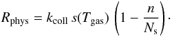
Atoms from a gas at temperature Tgas collide with the grain at a rate
kcoll =
πa2n(H)
vth, where
 is the thermal velocity. We call
s(Tgas) the sticking
probability and discuss later our choice for this function. The probability to land on
an empty site is
is the thermal velocity. We call
s(Tgas) the sticking
probability and discuss later our choice for this function. The probability to land on
an empty site is  and the physisorption rate is thus
 We assume that gas atoms falling on an
occupied site are never rejected and react with the adsorbed atom to form a
H2 molecule,
which is immediately desorbed by the formation energy. This assumption of
Eley-Rideal-like reaction for physisorbed atoms is similarly made in the model of Cuppen et al. (2006) with the difference that they do
not consider desorption at the formation of the new molecule. This direct Eley-Rideal
process is expected to have a large cross section at temperatures relevant to the
interstellar medium (Martinazzo & Tantardini
2006), and it is thus a reasonable assumption to assume that it dominates over
rejection. To estimate the influence of this assumption on our results, we computed the
contribution of this direct ER-like reaction process to the total mean formation rate
through physisorption and found it to be a negligible fraction (always less than 1% of
the total average formation rate). Despite the very small contribution of this
Eley-Rideal-like process to the physisorption-based formation rate in our model, we keep
calling the physisorption-based mechanism LH mechanism to distinguish it from the
chemisorption-based ER mechanism.
We assume that gas atoms falling on an
occupied site are never rejected and react with the adsorbed atom to form a
H2 molecule,
which is immediately desorbed by the formation energy. This assumption of
Eley-Rideal-like reaction for physisorbed atoms is similarly made in the model of Cuppen et al. (2006) with the difference that they do
not consider desorption at the formation of the new molecule. This direct Eley-Rideal
process is expected to have a large cross section at temperatures relevant to the
interstellar medium (Martinazzo & Tantardini
2006), and it is thus a reasonable assumption to assume that it dominates over
rejection. To estimate the influence of this assumption on our results, we computed the
contribution of this direct ER-like reaction process to the total mean formation rate
through physisorption and found it to be a negligible fraction (always less than 1% of
the total average formation rate). Despite the very small contribution of this
Eley-Rideal-like process to the physisorption-based formation rate in our model, we keep
calling the physisorption-based mechanism LH mechanism to distinguish it from the
chemisorption-based ER mechanism.
Surface atoms can then evaporate. The adsorbed atoms are assumed to be thermalized at
the grain temperature and must overcome the well energy Ephys. We take
this desorption rate for one atom to be of the form
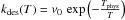 , where T is the grain
temperature, Tphys =
Ephys/k, and
ν0 is a typical vibration frequency
taken as
, where T is the grain
temperature, Tphys =
Ephys/k, and
ν0 is a typical vibration frequency
taken as  with a typical size d0 = 0.1 nm
(Hasegawa et al. 1992). The total desorption
rate on the grain is then
with a typical size d0 = 0.1 nm
(Hasegawa et al. 1992). The total desorption
rate on the grain is then 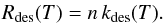 To migrate from site to site, an atom must
cross a barrier of height Emigr. It can do so by thermal hopping
or by tunneling for which we use the formula from Le
Bourlot et al. (2012). The migration rate for one physisorbed atom is thus
To migrate from site to site, an atom must
cross a barrier of height Emigr. It can do so by thermal hopping
or by tunneling for which we use the formula from Le
Bourlot et al. (2012). The migration rate for one physisorbed atom is thus
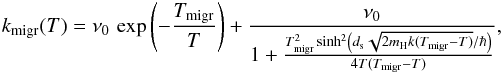 where Tmigr =
Emigr/k.
where Tmigr =
Emigr/k.
The main formation process is the meeting of two physisorbed atoms during a migration
event. In a simple approximation (see Lohmar & Krug
2006; Lohmar et al. 2009, for a more
detailed treatment of the sweeping rate), we take this formation rate to be
 We also take direct reaction of a
physisorbed atom with a gas atom in an ER-like mechanism into account, with a rate
We also take direct reaction of a
physisorbed atom with a gas atom in an ER-like mechanism into account, with a rate
 This term is only significant for very low
dust temperatures (a few K,
depending on the collision rate with gas atoms).
This term is only significant for very low
dust temperatures (a few K,
depending on the collision rate with gas atoms).
We assume immediate desorption of the newly formed molecule because of the high formation energy compared to the binding energy, thus making a similar assumption to recent models (Iqbal et al. 2012; Le Bourlot et al. 2012). Experimental results indicate that a small fraction of the formed molecules may stay on the surface at formation (Katz et al. 1999; Perets et al. 2007). Theoretical studies (Morisset et al. 2004a, 2005) suggest that even when the formed molecule does not desorb immediately at formation, it desorbs after a few picoseconds by interacting with the surface due to its high internal energy. It is thus equivalent to immediate desorption compared to the timescales of the other events.
Model parameters for physisorption.
If the temperature fluctuations are neglected, an equilibrium surface population can be
computed using the equilibrium rate equation  (the factor of 2 comes from the fact
that one formation through migration event reduces the population by two). We find
(the factor of 2 comes from the fact
that one formation through migration event reduces the population by two). We find
![Mathematical equation: \begin{eqnarray} n_{\rm eq}(T)&=&\frac{\left(1+s(T_{\mathrm{gas}})\right)k_{\mathrm{coll}}}{4\, k_{\mathrm{mig}}(T)}\left(1+\frac{N_{\mathrm{s}}\, k_{\mathrm{des}}(T)}{k_{\mathrm{coll}}(1+s(T_{\mathrm{gas}}))}\right) \notag\\&&\quad\times \left[\sqrt{1+\frac{8N_{\mathrm{s}}\, k_{\mathrm{mig}}(T)\, s(T_{\mathrm{gas}})}{k_{\mathrm{coll}}(1+s(T_{\mathrm{gas}}))^{2}}\frac{1}{\left(1+\frac{N_{\mathrm{s}}\, k_{\mathrm{des}}(T)}{k_{\mathrm{coll}}(1+s(T_{\mathrm{gas}}))}\right)^{2}}}-1\right],\label{eq:n_eq_LH} \end{eqnarray}](/articles/aa/full_html/2014/09/aa22101-13/aa22101-13-eq64.png) (2)and the corresponding equilibrium formation
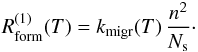
rate on one grain at temperature T is
(2)and the corresponding equilibrium formation
rate on one grain at temperature T is ![Mathematical equation: \begin{equation} r_{\mathrm{H}_{2}}^{\mathrm{eq}}(T)=k_{\mathrm{migr}}(T)\frac{[n_{\mathrm{eq}}(T)]^{2}}{N_{\mathrm{s}}}+k_{\mathrm{coll}}\frac{n_{\mathrm{eq}}(T)}{N_{\mathrm{s}}}\cdot\label{eq:rH2_eq_LH} \end{equation}](/articles/aa/full_html/2014/09/aa22101-13/aa22101-13-eq65.png) (3)Once again this expression is not valid for
a fluctuating temperature and the full calculation is described in the next Sect. 2.2.
(3)Once again this expression is not valid for
a fluctuating temperature and the full calculation is described in the next Sect. 2.2.
For the binding and migration energies, we use the values given in Table 1 associated to different substrates.
Many different expressions of the sticking coefficient have been given in the
literature. For simplicity, we use the same sticking probability for the
physisorption-based LH mechanism and the chemisorption-based ER mechanism, except for
the additional presence of a barrier in the ER case. We use the expression from Le Bourlot et al. (2012):
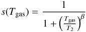 using T2 = 464 K and
β = 1.5,
which gives results close to the expression of Sternberg
& Dalgarno (1995).
using T2 = 464 K and
β = 1.5,
which gives results close to the expression of Sternberg
& Dalgarno (1995).
We also simply assume an equipartition of the formation energy among the kinetic energy of the newly formed molecule, its excitation energy, and the heating of the grain.
The total volumic H2 formation rate is often parametrized as
RH2
=
RfnHn(H)
to factor out the dependency to the atomic H abundance n(H) and to the dust abundance, which is
proportional to the total proton density nH, coming from the collision rate
between gas H atoms and dust
grains. The standard value of Rf is 3 × 10-17cm3
s-1. We also use the formation efficiency defined for one
grain as  , which represents the fraction of the
H atoms colliding with the
grain that are turned into H2.
, which represents the fraction of the
H atoms colliding with the
grain that are turned into H2.
2.1.3. Surface chemistry via Eley-Rideal mechanism
We also consider the chemisorption-based ER mechanism. The H atoms of the gas phase that hit the grain can bind to the surface by a covalent bond after overcoming a repulsive barrier. This process is called chemisorption (see for instance Jeloaica & Sidis 1999). Once chemisorbed, the atoms either evaporate and return to the gas phase, or react if another gas H atom lands on the same adsorption site.
We assume the chemisorption sites to be similarly distributed with the same inter-site distance ds = 0.26 nm. Each site is a potential well of depth Echem and is separated from the free state by a potential barrier of height Ebarr.
The collision rate kcoll is the same as in the LH case.
However, we have to take the presence of the chemisorption barrier into acount in the
sticking coefficient. Following Le Bourlot et al.
(2012), we use a sticking probability 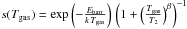 , where the second term accounts for
rebound of high energy atoms without sticking with Tbarr =
Ebarr/k = 300 K,
T2 =
464 K, and β = 1.5. The energy barrier for chemisorption on
perfect graphitic surfaces has been found to be of the order of 0.15−0.2 eV (but adsorption in para-dimer
configuration has a much lower barrier of 0.04 eV) (Sha
& Jackson 2002; Kerwin & Jackson
2008). As discussed in Le Bourlot et al.
(2012), the choice made here of a lower barrier for chemisorption is based on
the idea that real grain surfaces are not perfect flat surfaces like graphite, but
present a large number of defects. Surface defects are expected to induce a strongly
reduced barrier for chemisorption (Ivanovskaya et al.
2010; Casolo et al. 2013). Edge sites on
PAHs behave in a similar way (Bonfanti et al.
2011). Moreover, Mennella (2008) found
that chemisorption in aliphatic CH2,3 groups could also lead to efficient Eley-Rideal
formation with a very low chemisorption barrier.
, where the second term accounts for
rebound of high energy atoms without sticking with Tbarr =
Ebarr/k = 300 K,
T2 =
464 K, and β = 1.5. The energy barrier for chemisorption on
perfect graphitic surfaces has been found to be of the order of 0.15−0.2 eV (but adsorption in para-dimer
configuration has a much lower barrier of 0.04 eV) (Sha
& Jackson 2002; Kerwin & Jackson
2008). As discussed in Le Bourlot et al.
(2012), the choice made here of a lower barrier for chemisorption is based on
the idea that real grain surfaces are not perfect flat surfaces like graphite, but
present a large number of defects. Surface defects are expected to induce a strongly
reduced barrier for chemisorption (Ivanovskaya et al.
2010; Casolo et al. 2013). Edge sites on
PAHs behave in a similar way (Bonfanti et al.
2011). Moreover, Mennella (2008) found
that chemisorption in aliphatic CH2,3 groups could also lead to efficient Eley-Rideal
formation with a very low chemisorption barrier.
Finally, only atoms arriving on an empty adsorption site stick, corresponding to a
probability , where n is the number of
chemisorbed atoms.
Model parameters for chemisorption.
The chemisorption rate is thus 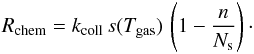 Atoms hitting an occupied site react with
the adsorbed atom to form a H2 molecule. Some theoretical studies show a very small
activation barrier of 9.2
meV (Morisset et al. 2004b)
for this reaction, but the existence of this barrier is under debate (Rougeau et al. 2011). To stay consistent with the
model of Le Bourlot et al. (2012) to which we
compare our results in Sect. 5, we neglect this
barrier compared to the stronger adsorption barrier. We found that including it in the
model reduces the formation efficiency by less than 10% in the range of gas temperatures where
the ER mechanism is important compared to the physisorption-based LH mechanism.
Atoms hitting an occupied site react with
the adsorbed atom to form a H2 molecule. Some theoretical studies show a very small
activation barrier of 9.2
meV (Morisset et al. 2004b)
for this reaction, but the existence of this barrier is under debate (Rougeau et al. 2011). To stay consistent with the
model of Le Bourlot et al. (2012) to which we
compare our results in Sect. 5, we neglect this
barrier compared to the stronger adsorption barrier. We found that including it in the
model reduces the formation efficiency by less than 10% in the range of gas temperatures where
the ER mechanism is important compared to the physisorption-based LH mechanism.
As the formation reaction releases 4.5
eV, which is much more than the binding energy, we assume that the
new molecule is immediately released in the gas. The formation rate is then
 Last, chemisorbed atoms can evaporate. This
effect is usually negligible at typical grain temperatures, but the fluctuating
temperatures of small grains can easily make excursions into the domain where
evaporation is significant. The adsorbed atoms are supposed to be thermalized at the
grain temperature, and must overcome the well energy Echem. The
desorption process is similar to the LH case, and we take again
Last, chemisorbed atoms can evaporate. This
effect is usually negligible at typical grain temperatures, but the fluctuating
temperatures of small grains can easily make excursions into the domain where
evaporation is significant. The adsorbed atoms are supposed to be thermalized at the
grain temperature, and must overcome the well energy Echem. The
desorption process is similar to the LH case, and we take again
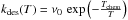 , where Tchem =
Echem/k, and
, where Tchem =
Echem/k, and
 (with d0 = 0.1 nm).
The total desorption rate on the grain is then Theoretical studies find the chemisorption
energy on graphene to be in the range 0.67−0.9 eV (Sha & Jackson
2002; Lehtinen et al. 2004; Casolo et al. 2009). On small PAHs, Bonfanti et al. (2011) find binding energies in the
range 1−3 eV for edge sites
and in the range 0.5−1 eV
for non edge sites. In this overall range 5800 −35 000 K, we choose a low value of 7000 K
to estimate the maximum effect of temperature fluctuations on the ER mechanism.
(with d0 = 0.1 nm).
The total desorption rate on the grain is then Theoretical studies find the chemisorption
energy on graphene to be in the range 0.67−0.9 eV (Sha & Jackson
2002; Lehtinen et al. 2004; Casolo et al. 2009). On small PAHs, Bonfanti et al. (2011) find binding energies in the
range 1−3 eV for edge sites
and in the range 0.5−1 eV
for non edge sites. In this overall range 5800 −35 000 K, we choose a low value of 7000 K
to estimate the maximum effect of temperature fluctuations on the ER mechanism.
We sum up the model parameters in Table 2.
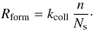
When neglecting the fluctuations of the grain temperature, we can calculate the
equilibrium surface population neq using the equilibrium rate
equation Rchem −
Rform −
Rdes(T) = 0, which
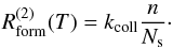
gives 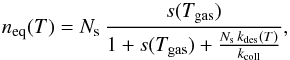 (4)and the corresponding equilibrium formation
rate on one grain at temperature T is
(4)and the corresponding equilibrium formation
rate on one grain at temperature T is 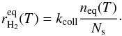 (5)However, when temperature fluctuations are
taken into account, this equilibrium situation is not valid. The method we use to
calculate this effect is described in Sect. 2.2.
(5)However, when temperature fluctuations are
taken into account, this equilibrium situation is not valid. The method we use to
calculate this effect is described in Sect. 2.2.
The energy liberated from the formation reaction is split between the excitation and kinetic energy of the molecule and the heating of the grain. As in Le Bourlot et al. (2012), we take the results of Sizun et al. (2010) for the ER mechanism : 2.7 eV goes into the excitation energy of the molecule, 0.6 eV into its kinetic energy, and 1 eV is given to the grain.
We must note that the part of the formation energy given to the grain creates another coupling between surface population and grain temperature. This fraction of the formation energy (1 eV) is not completely negligible compared to photon energies. This additional retro-coupling between surface chemistry and temperature is ignored in the statistical calculation presented in this article. However, its effect on the equilibrium situation when neglecting fluctuations is evaluated in Appendix A. It is found to be negligible as the power given to the grain is usually much smaller that the radiative power it receives.
We can again define the formation parameter Rf as RH2 =
RfnHn(H)
and the formation efficiency for one grain as .
2.2. Method
To take into account temperature fluctuations, we adopt a statistical point of view, and we describe the statistical properties of the fluctuating variables.
The necessary statistical information on our system is contained in the probability density function (PDF) f(X), giving the probability to find the system in the state X that is defined by the two variables E, the thermal energy of the grain (equivalent to its temperature T), and n, the number of adsorbed H atoms on its surface. The function f is thus the joint PDF in the two variables. As we treat our two formation mechanisms independently, n counts chemisorbed or physisorbed atoms depending on which mechanism we are discussing.
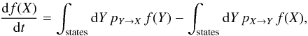
The time evolution of this PDF is governed by the master equation:
 where pX →
Y is the transition rate from state
X to
Y. This
equation expresses that the probability of being in a given state varies in time due to
the imbalance between the rate of arrivals and the rate of departures. In a stationary
situation, the two rates, which we call as the gain and loss rates respectively, must
compensate each other.
where pX →
Y is the transition rate from state
X to
Y. This
equation expresses that the probability of being in a given state varies in time due to
the imbalance between the rate of arrivals and the rate of departures. In a stationary
situation, the two rates, which we call as the gain and loss rates respectively, must
compensate each other.
We are thus looking for a solution to the equation 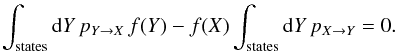 Two different kinds of transitions occur: the
emission or absorption of a photon, which changes only the thermal energy E of the grain, and the
adsorption, desorption, or reaction of hydrogen atoms, which changes only the surface
population n.
The two variables are only coupled by the transition rates for the chemical events, which
depend on the grain temperature. The population fluctuations are thus entirely driven by
the temperature fluctuations with no retroactions (as mentioned before we neglect grain
heating by the formation process).
Two different kinds of transitions occur: the
emission or absorption of a photon, which changes only the thermal energy E of the grain, and the
adsorption, desorption, or reaction of hydrogen atoms, which changes only the surface
population n.
The two variables are only coupled by the transition rates for the chemical events, which
depend on the grain temperature. The population fluctuations are thus entirely driven by
the temperature fluctuations with no retroactions (as mentioned before we neglect grain
heating by the formation process).
As the transition mechanisms modify only one variable at a time, we split each of the
gain and loss terms into two parts, respectively for photon processes (affecting only
E) and for
surface chemical processes (affecting only n),  (6)with
 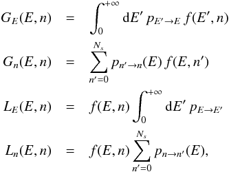 where we have simplified the notations for
the transition rates as transitions only affect one variable at a time and the transitions
affecting E
(photon absorptions or emissions) have rates that are independent of n.
where we have simplified the notations for
the transition rates as transitions only affect one variable at a time and the transitions
affecting E
(photon absorptions or emissions) have rates that are independent of n.
We now first show how the thermal energy marginal PDF fE(E) (or the equivalent temperature PDF fT(T)) can be derived from our formalism, which reduces to equations similar to previous works (Desert et al. 1986; Draine & Li 2001). We then show how the formation rates in the LH case and in the ER case can be derived.
2.2.1. Thermal energy PDF
Summing Eq. (6) over all
n values,
we obtain 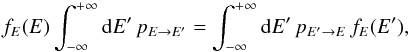 (7)where fE(E) = ∑
nf(E,n)
is the marginal PDF for the single variable E. The marginal PDF fE can easily be
converted into a grain temperature PDF fT through the
relationship
(7)where fE(E) = ∑
nf(E,n)
is the marginal PDF for the single variable E. The marginal PDF fE can easily be
converted into a grain temperature PDF fT through the
relationship 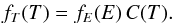 We thus obtain an independent master
equation for the temperature fluctuations.
We thus obtain an independent master
equation for the temperature fluctuations.
Detailing the transition rates in Eq. (7), we can rewrite it as 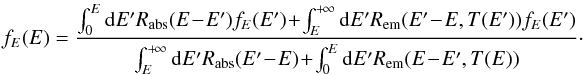 (8)This equation is an eigenvector equation
for the linear integral operator defined by the right-hand side: fE(E) = ℒ [
fE ]
(E). A stationary PDF for the grain thermal energy
is a positive and normalized eigenvector of this operator for the eigenvalue
1. The existence and
unicity of this eigenvector is proven in Appendix B. Moreover, the other eigenvalues all have real parts that are lower than
1 (see Appendix B). We can thus converge toward the solution by
building a sequence ℒn [ fE
] (the exponent refers to operator composition) from an initial
guess. We solve this equation numerically by choosing an energy grid {Ei} and solving for
piecewise linear functions on this grid.
(8)This equation is an eigenvector equation
for the linear integral operator defined by the right-hand side: fE(E) = ℒ [
fE ]
(E). A stationary PDF for the grain thermal energy
is a positive and normalized eigenvector of this operator for the eigenvalue
1. The existence and
unicity of this eigenvector is proven in Appendix B. Moreover, the other eigenvalues all have real parts that are lower than
1 (see Appendix B). We can thus converge toward the solution by
building a sequence ℒn [ fE
] (the exponent refers to operator composition) from an initial
guess. We solve this equation numerically by choosing an energy grid {Ei} and solving for
piecewise linear functions on this grid.
2.2.2. Eley-Rideal mechanism
We first present the method for the ER mechanism as the linearity of the chemical rates in n simplifies the problem significantly. We can avoid directly solving the full master equation for the joint PDF in two variables (Eq. (6)).
We are interested in the average ER formation rate
 Knowing fE(E),
we can rewrite it as:
Knowing fE(E),
we can rewrite it as: 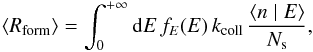 where
where
 is the conditional expectation of the
surface population at thermal energy E. It is by definition the expected value (or
ensemble average) of the surface population of a grain, knowing that
this grain has thermal energy E. Multiplying Eq. (6) by n and summing over all n values gives the
equation governing this quantity ⟨n | E⟩,
is the conditional expectation of the
surface population at thermal energy E. It is by definition the expected value (or
ensemble average) of the surface population of a grain, knowing that
this grain has thermal energy E. Multiplying Eq. (6) by n and summing over all n values gives the
equation governing this quantity ⟨n | E⟩, 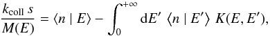 (9)where
 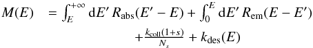 and
and ![Mathematical equation: \begin{eqnarray*} K(E,E')=\begin{cases} {\displaystyle \frac{f_{E}(E')\, R_{\mathrm{abs}}(E-E')}{f_{E}(E)\, M(E)}} & \mathrm{if}\qquad E'\in[0,E]\\ \\ {\displaystyle \frac{f_{E}(E')\, R_{\mathrm{em}}(E'-E,T(E'))}{f_{E}(E)\, M(E)}} & \mathrm{if}\qquad E'>E. \end{cases} \end{eqnarray*}](/articles/aa/full_html/2014/09/aa22101-13/aa22101-13-eq128.png) After a similar discretization, this is a
linear system of equations. However, while being nonsingular, it converges exponentially
fast toward a singular system as the grain size a grows, making standard
numerical procedures unusable.
After a similar discretization, this is a
linear system of equations. However, while being nonsingular, it converges exponentially
fast toward a singular system as the grain size a grows, making standard
numerical procedures unusable.
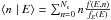
To avoid this problem, we rewrite this equation. Multiplying by M(E)fE(E)
and integrating it over E yields ![Mathematical equation: \begin{equation} k_{\mathrm{coll}}\, s=\int_{0}^{+\infty}{\rm{d}}E'\left[\frac{k_{\mathrm{coll}}(1+s)}{N_{s}}+k_{\mathrm{des}}(E')\right]f_{E}(E')\,\left\langle n\mid E'\right\rangle .\label{eq:norm_ER} \end{equation}](/articles/aa/full_html/2014/09/aa22101-13/aa22101-13-eq130.png) (10)Dividing again by M(E) and
subtracting it from the initial equation gives
(10)Dividing again by M(E) and
subtracting it from the initial equation gives 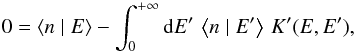 (11)where
 . This is again an eigenvector equation
for the eigenvalue 1 of a
linear integral operator. After discretization, we numerically compute this eigenvector
and use Eq. (10) as a normalization
condition. This procedure proved to work on the entire range of relevant grain sizes.
. This is again an eigenvector equation
for the eigenvalue 1 of a
linear integral operator. After discretization, we numerically compute this eigenvector
and use Eq. (10) as a normalization
condition. This procedure proved to work on the entire range of relevant grain sizes.
2.2.3. Langmuir-Hinshelwood mechanism
For the LH mechanism, the formation rate contains a quadratic term. When trying to
apply a similar method to the LH mechanism, the equivalent of Eq. (11) is then an infinite system of equations
on the conditional moments of the population ⟨n | E⟩,
 ,
,  We thus directly solve the main master
equation (Eq. (6)), despite the
computational burden.
We thus directly solve the main master
equation (Eq. (6)), despite the
computational burden.
Writing explicitly the transition rates in Eq. (6), we get ![Mathematical equation: \begin{eqnarray} \label{eq:LH-master-raw} 0&=&\int_{0}^{E}{\rm{d}}E'\, R_{\rm abs}(E-E')\, f(E',n) \notag\\ &&\quad +\int_{E}^{+\infty}{\rm{d}}E'\, R_{\rm em}(E'-E,T(E'))\, f(E',n) \notag\\ &&\quad +f(E,n-1)k_{\rm coll}s(T_{\rm gas})\left(1-\frac{n-1}{N_{\rm s}}\right) \notag\\ &&\quad +f(E,n+1)\left[(n+1)\, k_{\rm des}(T)+k_{\rm coll}\frac{n+1}{N_{\rm s}}\right]\notag\\ &&\quad +f(E,n+2)k_{\rm mig}(T)\frac{(n+2)(n+1)}{N_{\rm s}} \notag\\ &&\quad -\left[\int_{E}^{+\infty}{\rm{d}}E'\, R_{\mathrm{\rm abs}}(E'-E)+\int_{0}^{E}{\rm{d}}E'\, R_{\mathrm{\rm em}}(E-E')\right]\, f(E,n) \notag\\ &&\quad -f(E,n)\left[k_{\rm coll}s(T_{\rm gas})\left(1-\frac{n}{N_{\rm s}}\right)+n\, k_{\rm des}(T)+k_{\rm coll}\frac{n}{N_{\rm s}}\right. \notag\\ &&\quad \left.+k_{\rm mig}(T)\frac{n(n-1)}{N_{\rm s}}\right], \end{eqnarray}](/articles/aa/full_html/2014/09/aa22101-13/aa22101-13-eq137.png) (12)where, as boundary conditions, all
expressions n −
1, n +
1 and n +
2 are implicitly taken to be 0 if they become negative or greater
than Ns.
(12)where, as boundary conditions, all
expressions n −
1, n +
1 and n +
2 are implicitly taken to be 0 if they become negative or greater
than Ns.
We define the total loss rate as 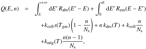 the integral operator (for photon induced
transitions) as
the integral operator (for photon induced
transitions) as &=&\int_{0}^{E}{\rm{d}}E'\, R_{\rm abs}(E-E')\, f(E',n)\\ &&\quad +\int_{E}^{+\infty}{\rm{d}}E'\, R_{\rm em}(E'-E,T(E'))\, f(E',n), \end{eqnarray*}](/articles/aa/full_html/2014/09/aa22101-13/aa22101-13-eq143.png) and the discrete jump operator (for
chemical transitions) as
and the discrete jump operator (for
chemical transitions) as &=& f(E,n-1)k_{\rm coll}s(T_{\rm gas})\left(1-\frac{n-1}{N_{\rm s}}\right)\\ &&\quad +f(E,n+1)\left[(n+1)\, k_{\rm des}(T)+k_{\rm coll}\frac{n+1}{N_{\rm s}}\right]\\ &&\quad +f(E,n+2)k_{\rm mig}(T)\frac{(n+2)(n+1)}{N_{\rm s}}\cdot \end{eqnarray*}](/articles/aa/full_html/2014/09/aa22101-13/aa22101-13-eq144.png) We can then rewrite Eq. (12)in a simplified form as
We can then rewrite Eq. (12)in a simplified form as +\mathcal{J}[f](E,n)\right].\label{eq:LH-master-simple} \end{equation}](/articles/aa/full_html/2014/09/aa22101-13/aa22101-13-eq145.png) (13)This is an eigenvector equation for the
eigenvalue 1, which is
formally similar to Eq. (8). For the
same reasons as previously, we expect the operator defined by the right hand side to
have all its eigenvalues with real parts that are strictly lower than 1, except the
eigenvalue 1, which is simple. We can thus find the solution by iterating the
application of the operator from an initial guess.
(13)This is an eigenvector equation for the
eigenvalue 1, which is
formally similar to Eq. (8). For the
same reasons as previously, we expect the operator defined by the right hand side to
have all its eigenvalues with real parts that are strictly lower than 1, except the
eigenvalue 1, which is simple. We can thus find the solution by iterating the
application of the operator from an initial guess.
The equation is solved numerically using this iterative procedure. The computation time is found to explode when increasing the grain size a. In addition to the number of possible values of n increasing as a2, the number of iterations necessary to converge toward the stationary solution is also found to quickly increase with a. Grouping the values of n in bins to reduce the matrix size does not solve the problem, as the reduction of the computation time due to the smaller matrices is found to be balanced by a roughly equivalent increase in the number of iterations necessary to converge to a given stationarity threshold.
We can thus only use this method up to moderate grain sizes (~20 nm with 2 days of computation). In later sections, we see, however, that this is sufficient to observe the range of sizes for which the temperature fluctuations significantly impact the chemistry. In addition, a much quicker yet sufficiently accurate approximation is presented in Sect. 3.
3. Approximations
In this section, we construct fast approximations of the formation rate based on simple physical arguments and compare their results with those of the exact method presented in Sect. 2.2. An approximation is especially necessary for the LH mechanism to avoid the prohibitive computational cost of the exact method. A similar approximation is given for completeness for the ER mechanism. Those methods assume the temperature PDF fT(T) to be known. It can be computed, for instance, by the method described in Sect. 2.2.1.
3.1. Approximation of the Langmuir-Hinshelwood formation rate
We build our method around an approximation of ⟨n|T⟩, the average population on the grains that are at a given temperature T. We first write a balance equation for this average population, taking into account both chemical processes (changing only the grain’s population), and grains leaving or reaching this temperature T.
We first consider the chemical processes. Those are described in Sect. 2.1.2:
-
The grain can gain atoms through adsorption (average rate
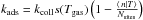 ).
). -
The grain can lose atoms through desorption (rate ⟨n|T⟩kdes(T)).
-
The grain can lose atoms through LH reaction, a term we express later. For now, let us write it as
 . We discuss this term in depth
below.
. We discuss this term in depth
below. -
The grain can lose atoms through direct ER reaction (rate
 ).
).
On the other hand, the grain can also leave the temperature T. At equilibrium, the rate at which grains leave the state T is exactly balanced by the rate of arrivals from other states. The net effect on the conditional average ⟨n|T⟩ can be a loss or a gain depending on whether the average population of the grains arriving from other states is higher or lower than ⟨n|T⟩. In general, noting kleave(T), the rate at which grains leave the state T, and ⟨narrivals|T⟩, the average population on grains arriving in state T, the net gain rate is kleave(T)(⟨narrivals|T⟩ − ⟨n|T⟩).
Up to now, no approximation has been made.
As we expected high temperatures states, where desorption dominates all other processes, to have negligible formation and extremely low average population, we focus our approximation on a low temperature regime.
We want to estimate what fraction of the grains leaving state T will come back bare (or
with a negligible population compared to ⟨n|T⟩). We make the following
approximation: grains leaving T to reach the regime where desorption dominates,
come back with no population. Fluctuations that do not reach the desorption regime leave
the surface population unchanged. We define the temperature Tlim that
delimits these regimes as the temperature at which the desorption rate for one atom
becomes equal to the adsorption rate for the grain (we call Elim the
corresponding thermal energy): 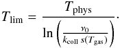 We thus define
 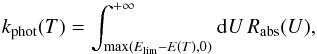 (14)the rate at which grains leave state
T to reach
a temperature above the limit. The net loss rate due to fluctuations is then
kphot(T)⟨n|T⟩.
(14)the rate at which grains leave state
T to reach
a temperature above the limit. The net loss rate due to fluctuations is then
kphot(T)⟨n|T⟩.
We have thus obtained a rate equation for the conditional average population at
temperature T: 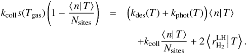 (15)This equation is in closed form if we can
express as a function of ⟨n|T⟩
only. We distinguish the two regimes ⟨n|T⟩ > 1 and ⟨n|T⟩ <
1. From now on, we simplify the notations by noting s =
s(Tgas).
(15)This equation is in closed form if we can
express as a function of ⟨n|T⟩
only. We distinguish the two regimes ⟨n|T⟩ > 1 and ⟨n|T⟩ <
1. From now on, we simplify the notations by noting s =
s(Tgas).
3.1.1. Regime with ⟨n|T⟩ > 1
In this regime, we assume that the discrete nature of the number of surface atoms is
negligible and treat this variable as continuous. We then have
 . We also know that when ⟨n|T⟩ ≫
1, direct ER reaction is likely to dominate so that a precise
determination of the LH reaction rate is not necessary. We thus make the simple
approximation ⟨n2|T⟩ =
⟨n|T⟩2. Using this
approximation in Eq. (15), we then get
. We also know that when ⟨n|T⟩ ≫
1, direct ER reaction is likely to dominate so that a precise
determination of the LH reaction rate is not necessary. We thus make the simple
approximation ⟨n2|T⟩ =
⟨n|T⟩2. Using this
approximation in Eq. (15), we then get
![Mathematical equation: \begin{eqnarray} \left\langle \left.n\right|T\right\rangle &=&\frac{1+s}{4}\frac{k_{\rm coll}}{k_{\rm mig}(T)}\left(1+\frac{N_{\rm sites}(k_{\rm des}(T)+k_{\rm phot}(T))}{k_{\rm coll}(1+s)}\right)\notag\\ &&\quad \times\left[\sqrt{1 \! + \! \frac{8s}{(1+s)^{2}}\frac{k_{\rm mig}(T)}{k_{\rm coll}}\frac{N_{\rm sites}}{\left(1+\frac{N_{\rm sites}(k_{\rm des}(T)+k_{\rm phot}(T))}{k_{\rm coll}(1+s)}\right)^{2}}}-1\right]\cdot \end{eqnarray}](/articles/aa/full_html/2014/09/aa22101-13/aa22101-13-eq169.png) (16)If this results becomes smaller than
1, we switch to the other
regime.
(16)If this results becomes smaller than
1, we switch to the other
regime.
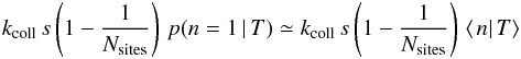
3.1.2. Regime with ⟨n|T⟩ < 1
In this regime, discretisation effects are very important. Formation is dominated by LH reaction, which can only happen if two atoms are present on the grain at the same time. We use reasoning that is similar to the modified rate equation approach developed by Garrod (2008).
As the average population is low, we can make the approximation ⟨n|T⟩ ≃
p(n = 1 | T),
where the right hand side is the conditional probability of having one surface atom
knowing that the temperature is T. The LH formation rate can then be computed the
following way. The formation rate is the rate at which gas atoms fall on a grain that
already had one adsorbed atom AND reaction occurs before any other process removes one
of the atoms. The first part of the sentence gives a rate
 using the previous approximation. Once we
have two atoms on the grain, the probability that they react before anything else
removes one atom is
using the previous approximation. Once we
have two atoms on the grain, the probability that they react before anything else
removes one atom is 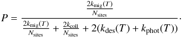 This gives
 We inject this expression in Eq. (15)and finally find the solution for this
regime:
We inject this expression in Eq. (15)and finally find the solution for this
regime: 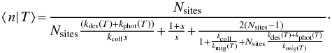 (17)
(17)
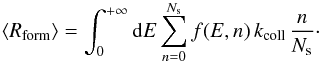
3.1.3. Total formation rate
The total formation rate is then computed by integrating over the temperature PDF
f(T) and distinguishing the two
regimes: 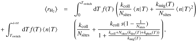 (18)where Tswitch is the
temperature at which ⟨n|T⟩ becomes <1 (⟨n|T⟩ >
1 for T<Tswitch, and
⟨n|T⟩
< 1 for T>Tswitch).
(18)where Tswitch is the
temperature at which ⟨n|T⟩ becomes <1 (⟨n|T⟩ >
1 for T<Tswitch, and
⟨n|T⟩
< 1 for T>Tswitch).
This approximation is compared to the exact method of Sect. 2.2.3 in Appendix C. It is found to give a very accurate estimate of the total average formation rate (within at most 6%). This approximation is used in all results shown in the following sections as the exact method is not practically usable.
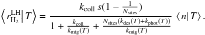
3.2. Approximation of the Eley-Rideal formation rate
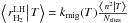
A similar approximation can be constructed in the case of the ER mechanism. We again
write a rate equation for the conditional average ⟨n|T⟩,
including a fluctuation loss term. We use the same approximation for this loss term with
the limiting temperature being 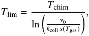 and the loss rate being kphot(T)⟨n|T⟩
with kphot(T) as defined as
previously by Eq. (14). The resulting rate
equation is then directly obtained in closed form:
and the loss rate being kphot(T)⟨n|T⟩
with kphot(T) as defined as
previously by Eq. (14). The resulting rate
equation is then directly obtained in closed form: 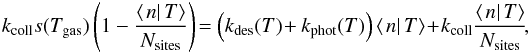 and no further approximation is needed. The
solution is
and no further approximation is needed. The
solution is 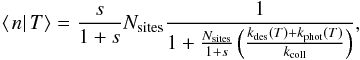 and the average H2 formation rate can then be
computed as
and the average H2 formation rate can then be
computed as 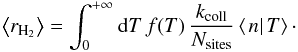 A comparison of this method with the exact
result is also performed in Appendix C. However, as
the exact method is easily tractable, the approximation is not used in the results
presented in the rest of this article.
A comparison of this method with the exact
result is also performed in Appendix C. However, as
the exact method is easily tractable, the approximation is not used in the results
presented in the rest of this article.
4. Results
The method described in the previous two sections was implemented as a stand alone code called Fredholm. The temperature PDF is computed using the exact method of Sect. 2.2.1 and the ER formation rate using the exact method of Sect. 2.2.2, while we use the approximation presented in Sect. 3 for the LH formation rate. This code is now used to study the effect of the temperature fluctuations on the formation rate and the influence of the external conditions (gas conditions and radiation field). We first present a few results on the temperature PDFs before presenting the results on H2 formation by the ER and LH mechanisms.
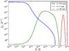 |
Fig. 1 Dust thermal energy PDFs for three grain sizes (amorphous carbon grains under a radiation field with G0 = 120). |
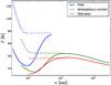 |
Fig. 2 Equilibrium temperature (dashed line) and actual average temperature (solid line), as a function of the grain size for the three types of grains (radiation field G0 = 120). |
4.1. Dust temperature probability density functions and grain emission
The thermal energy PDFs that we compute are shown in Fig. 1, which highlights the change of shape as we go from small grains to bigger grains. For small sizes, most of the grains are in the lowest energy states (the non-zero limit at zero energy can be easily derived from the master equation), while the high energy tail extends very far (the abrupt cut around 2 × 10-18 J is due to the Lyman cutoff present in the radiation field). As we go to bigger grains, the fraction of grains in the low energy plateau decreases, and the PDF takes a more peaked form but keeps a clear asymmetry. For the bigger sizes, the PDF becomes very sharp around its maximum and its relative width decreases towards zero, but the shape remains asymmetrical and could be asymptotically log-normal.
As expected, the average temperature converges toward the usual equilibrium temperature at large grain sizes but is significantly lower at small sizes, as shown in Fig. 2. High temperature grains have a much higher contribution to the average energy balance through their high emissivity. Thus, a very low fraction of high temperature grains is sufficient to lower the average temperature of the PDF compared to the equilibrium temperature. The temperature increase at very low grain sizes, which we can see on both the equilibrium and average temperatures, is due to the property that the smallest sizes have decreased cooling efficiency (as they cannot emit photons with higher energies than their own internal energy, their emission spectrum is reduced).
This part of the computation has been done before (Desert et al. 1986; Draine & Li 2001) and especially in the DustEM code (see Compiègne et al. 2011) to compute the infrared emission of dust. We checked the results of our code, which is named Fredholm, by comparing both the temperature PDFs, and the derived grain emissivity to the public DustEM code. We found a good agreement between the results, and despite small differences in the temperature PDFs (due mainly to the continuous cooling approximation in DustEM), the final emissivities are extremely close. Figure 3 shows the final comparison on a dust population corresponding to Compiègne et al. (2011) with PAHs, small carbonaceous grains, large carbonaceous grains, and large silicate grains.
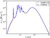 |
Fig. 3 Local dust emissivity (emitted power per unit of volume) as a function of wavelength for a dust population corresponding to Compiègne et al. (2011) under a radiation field with G0 = 100. We compare our code, Fredholm, with DustEM. |
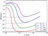 |
Fig. 4 Formation efficiency (LH mechanism) on one grain (carbonaceous) as a function of size for different radiation field intensities (in a gas at nH = 104 cm-3, T = 100 K). Solid lines: full computation. Dashed line: equilibrium rate equation results. The binding and barrier energies correspond to ices. |
4.2. H2 formation rate: LH mechanism
We apply the approximation method described in Sect. 3 to compute the H2 formation rate on physisorption sites. The results presented here concern unshielded gas in which the equilibrium rate equation method gives very inefficient LH formation rate due to high dust temperatures (i.e., PDR edges). For results in a more shielded gas, see Sect. 5 describing the coupling with full cloud simulations.
The results shown in this section use binding and barrier energies corresponding to either ices or amorphous carbon surfaces (see Table 1) as specified for each figure. Silicates have intermediate values and are thus not shown here. On the other hand, the optical and thermal properties of the grains are those of amorphous carbon grains.
We first show results for ice surfaces. Figure 4 shows the formation efficiency on one carbonaceous grain as a function of the grain size under various radiation field intensities and compares the equilibrium rate equation method with our estimation of the fluctuation effects. The results for small grains are different by several orders of magnitude; the method presented here giving a much more efficient formation. For large grains, the two methods converge as expected.
To understand those differences, we show how the temperature of a 3 nm dust grain is distributed compared to
the formation efficiency domain in Fig. 5. We show
both the efficiency curve that would be obtained from an equilibrium computation without
fluctuations (dashed line) and the true conditional mean efficiency
 (solid line), for fluctuating grains when
they are at the given temperature T. We see two different effects caused by the
fluctuations. First, the efficiency domain is reduced in both range and maximum value.
This occurs because grains do not stay in the low temperature regime but undergo frequent
fluctuations going to the high temperature domain where their surface population
evaporates quickly before cooling down. Their average coverage when they are at low
temperatures is thus decreased. The amplitude of this effect depends on the competition
between the fluctuation timescale and the adsorption timescale.
(solid line), for fluctuating grains when
they are at the given temperature T. We see two different effects caused by the
fluctuations. First, the efficiency domain is reduced in both range and maximum value.
This occurs because grains do not stay in the low temperature regime but undergo frequent
fluctuations going to the high temperature domain where their surface population
evaporates quickly before cooling down. Their average coverage when they are at low
temperatures is thus decreased. The amplitude of this effect depends on the competition
between the fluctuation timescale and the adsorption timescale.
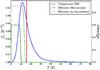 |
Fig. 5 Temperature PDF (blue line, left axis) for a 3 nm carbonaceous dust grain, as compared to the formation efficiency (LH mechanism) as a function of temperature (green lines, right axis). The red vertical line marks the mean temperature of the blue PDF. The grain receives a G0 = 20 radiation field and is surrounded by a 100 K gas with nH = 104 cm-3. The energy values correspond to ices. |
The other effect comes from the spread of the temperature PDF. While the average temperature of the PDF falls in the low efficiency domain (and the equilibrium temperature, being higher, is even worse), a significant part of the temperature PDF actually falls in the high efficiency domain, resulting in a quite efficient formation as seen in Fig. 4. The grain spends most of its time in the cold states and makes quick excursions into the high temperatures that shift the average toward high temperatures. The resulting formation rate is thus determined by the fraction of the time spent in the high efficiency domain and not by the equilibrium or average temperature of the grain. As described in Sect. 4.1, the smaller the grain, the more asymmetric the temperature PDF with most of the PDF below its average and a long high temperature tail. The smallest grains are thus the most affected, and we see (Fig. 4) that formation on the very small grains is significantly improved even for the highest radiation field intensities. As the radiation field intensity is decreased, larger grains are affected and become efficient. Grains up to 20 nm are affected. We note here that Cuppen et al. (2006) do not consider grains smaller than 5 nm and thus do not include part of the affected range; they, however, find a similar effect from 5 nm to ~10 nm on their flat surface model.
Parameters of the dust population.
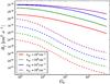 |
Fig. 6 Integrated formation rate parameter Rf (LH mechanism) for a carbonaceous dust population (see Table 3) as a function of the radiation field intensity G0 for different gas densities (the gas temperature is fixed at 100 K). Solid lines: full computation. Dashed lines: equilibrium rate equation results. Binding and barrier energies corresponding to ices. |
To evaluate the importance of this effect on the global formation rate, we integrate our formation rate on a MRN-like power law distribution (Mathis et al. 1977) of carbonaceous grains with an extended size range that goes from 1 nm to 0.3 μm (see Table 3) and obtain a volumic formation rate RH2.
As this distribution strongly favors small grains in term of surface, this integrated rate is strongly affected by the effect on small grains. Figure 6 shows this total formation rate as a function of the radiation field intensity for various gas densities (still using ice energy values). We obtain very efficient formation from the LH mechanism in unshielded PDR edge conditions for high gas densities. In all cases, the formation rate is increased by several orders of magnitude compared to the equilibrium computation. As the smallest grains remain efficient even for strong radiation fields, the total formation rate decreases more slowly when increasing the radiation field.
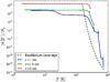 |
Fig. 8 Conditional mean of the surface coverage (chemisorption only) as a function of grain temperature for three sizes of amorphous carbon grains (solid lines) and equilibrium coverage (dashed line). The grain is surrounded by gas at density nH = 104 cm-3 and temperature T = 350 K under a radiation field with G0 = 120. |
Moreover, we note a difference in the dependency to the gas density. The gas density dependency that comes from the collision rate is already factored out in the definition of the Rf parameter shown on this graph. The equilibrium rate equation result is in the low efficiency regime, where the efficiency is determined by the competition between the adsorption rate (proportional to nH) and the desorption rate, and is thus proportional to the gas density. The result from the method presented here is mainly determined by the fraction of the time spend in the high efficiency regime. This fraction is fully determined by the photon absorption and emission processes and is independent of the gas density. The final result for high gas densities (nH> 103 cm-3) is thus largely independent of the gas density. For low densities, the reduction of the conditional average efficiency curve (noted in Fig. 5) becomes dominant. As this effect results from the competition between the fluctuation rate (due to photons) and the adsorption rate (proportional to nH), the resulting formation parameter Rf becomes proportional again to the gas density for low densities (nH< 103 cm-3). This change of behavior corresponds to the point where the fluctuation timescale becomes significantly smaller than the adsorption timescale.
Figure 7 shows the same result when using binding and barrier energies corresponding to amorphous carbon surfaces. As a consequence of the higher binding energy for amorphous carbon surface, the equilibrium result yields higher formation rates. The increase caused by the fluctuations is thus less dramatic but remains very large for strong radiation fields.
We can already note here that the formation rates obtained in those unshielded PDR edge conditions are comparable to the typical value of 3 × 10-17 cm3 s-1. The LH and the ER mechanisms thus become of comparable importance in PDR edges for high densities, as seen in the results of full cloud simulations shown in Sect. 5.
4.3. H2 formation rate: ER mechanism
The first step in our computation of the formation rate is the conditional mean of the surface population knowing the grain temperature. We show this quantity (as a fraction of the total number of sites) in Fig. 8, as compared to the coverage fraction for a grain at equilibrium at constant temperature (this equilibrium coverage fraction is independent of the grain size). As expected, the equilibrium coverage shows a plateau as long as the desorption rate is negligible compared to the adsorption rate. This plateau is lower than unity as the sticking is less than unity. Then the equilibrium coverage decreases as desorption becomes dominant. The dynamical effect of the temperature fluctuations has a consequence that the actual average populations are not at equilibrium. The grains undergoing a fluctuation to high temperature arrive in their new state with their previous population and then go through a transient desorption phase, which lasts a certain time, thus increasing the average population at the high temperatures compared to the equilibrium. When cooling down back to the low temperature states, re-accretion of their population takes some time, and this effect lowers the average population at low temperatures. Because this lowering effect is important, as seen in Fig. 8, it means that the characteristic time between two temperature spikes is sufficiently short compared to the adsorption timescale. The mechanism at play is thus that grains that go to high temperatures lose their population but then cool down faster than they re-adsorb their surface population and do not spend enough time in the low temperature state before the next fluctuation to have regained their equilibrium population. Of course, as the fluctuations are less dramatic for bigger grains (as a given photon energy makes a smaller temperature change: a Lyman photon at 912 Å brings a 1 nm grain to ~500 K but a 2 nm grain to only ~200 K), the effect disappears for larger grains, as seen in Fig. 8.
The formation rate on one grain is then simply  . The resulting formation efficiency on one
grain is shown in Fig. 9 as a function of grain size.
. The resulting formation efficiency on one
grain is shown in Fig. 9 as a function of grain size.
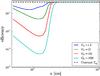 |
Fig. 9 H2 formation efficiency (ER mechanism) as a function of grain size for various radiation fields (carbonaceous grains in a gas at nH = 104 cm-3 and T = 350 K). |
As explained above, the smaller grains have a lower coverage than equilibrium due to temperature fluctuations and, thus, a decreased formation rate. Only grains below 2 nm are affected, as the same photon absorption causes a smaller temperature fluctuation for bigger grains. For stronger radiation fields, fluctuations occur with a shorter timescale, leaving less time for the surface population to reach equilibrium. The effect is then stronger and extends to higher sizes.
The affected range seems very small, but we have to remember that usual dust size distributions are such that the small grains represent most of the surface (e.g., the MRN distribution). Thus, the contribution from the smallest grain sizes dominates the global formation rate. By integrating over the dust size distribution (same as in Sect. 4.2), we obtain the volumic formation rate in the gas, which we can express as RH2 = Rfn(H) nH defining Rf. In the following, we compare the integrated formation rate that we obtain to the one obtained with the rate equation at constant temperature as used in Le Bourlot et al. (2012) and plot our results as a fraction of this reference formation rate.
The two main parameters are the radiation field intensity and the H atom collision rate (and the sticking coefficient, which modifies the effective collision rate). We use standard interstellar radiation fields with a scaling factor as explained in Sect. 2.1.1.
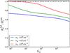 |
Fig. 10 Integrated formation rate Rf (ER mechanism) over a full dust size distribution (see Table 3) as a fraction of the equilibrium rate equation result. The result is shown for three different gas densities (thus changing the collision rate) as a function of the radiation field intensity. |
Figure 10 shows the effect of these two parameters. We show the formation rate as a function of the radiation field intensity for different gas densities to probe the effect of the collision rate. Note that the reference rate equation result at constant temperature does not depend on either of these parameters: the density dependency (from the collision rate) is eliminated in the definition of Rf, and the radiation field has no effect when the fluctuations are neglected (the equilibrium temperature is too low to trigger desorption). The effect we show is thus fully the effect of grain temperature fluctuations. As expected, the formation rate decreases when either the radiation intensity is increased or the collision rate is decreased, as the effect results from a competition between the fluctuation rate and the collision rate. The observed reduction remains limited and reaches a ~40% reduction or lower in the range of parameters that we explore. The result that an effect affecting only a tiny fraction of the range of grain sizes can have a significant effect on the integrated formation rate illustrates how the smallest sizes dominate the chemistry in the usual MRN size distribution.
The choice of the lower limit of this size distribution is thus of crucial importance. The lower this minimal size, the larger the usual equilibrium rate equation formation rate will be, as the total dust surface is increased for a constant total dust mass. However, as we lower this limit, we extend the range affected by the fluctuations, and thus obtain a stronger decrease compared to the rate equation result, as shown in Fig. 11. We observe no effect if the size distribution starts above the affected size (e.g., for amin = 3 nm), while a lower limit causes a stronger effect (up to ~60% with amin = 0.5 nm).
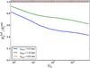 |
Fig. 11 Integrated formation rate ratio (ER mechanism) over a full dust size distribution, as a function of the radiation field intensity when changing the inferior limit of the grain size distribution (nH = 104 cm-3). |
Last, as noted in Sect. 2.1.3, the microphysical parameters of the adsorption process are not well known. The adsorption barrier affects the sticking and changes the effective collision rate (see Fig. 10 for the effect of the collision rate). The vibration frequency ν0 has a negligible effect in the range of reasonable values. The most important microphysical parameter is the chemisorption energy Tchem. Figure 12 shows the strong influence of this parameter on the result. A lower chemisorption energy allows for smaller fluctuations to trigger desorption. Bigger grains are thus affected, resulting in a much lower formation rate (e.g., a reduction of more than 90% for Tchem = 3500 K).
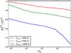 |
Fig. 12 Integrated formation rate ratio (ER mechanism) over a full dust size distribution, as a function of the radiation field intensity for different chemisorption binding energies (nH = 104 cm-3). |
5. Integration into the Meudon PDR code
We now investigate the effects of the changes in the formation rate found in the previous section on the overall structure and chemistry of an interstellar cloud with special attention to the observable line intensities.
Our code Fredholm, which computes the H2 formation rate from the LH and ER mechanisms as described in Sects. 2 and 3, has been coupled to the Meudon PDR code described in Le Petit et al. (2006).
The Meudon PDR code models stationary interstellar clouds in a 1D geometry with a full treatment of the radiative transfer (including absorption and emission by both gas and dust), thermal balance, and chemical equilibrium done in a self-consistent way. In its standard settings, the formation of H2 on dust grains is treated using rate equations and including both the LH and ER mechanism, as described in Le Bourlot et al. (2012). We have now enabled the possibility to compute the H2 formation rate using our code Fredholm from the gas conditions and the radiation field sent by the PDR code at each position in the cloud, thus taking temperature fluctuations into account. We compare the results of those coupled runs with the simpler rate equation treatment. The dust population in the PDR models presented here is a single component following a MRN-like power-law distribution from 1 nm to 0.3 μm with an exponent of −3.5, using properties corresponding to a 70−30% mix of graphites and silicates above 3 nm and a progressive transition to PAH properties from 3 nm to 1 nm.
A direct comparison between the rate equation approximation and a full account of stochastic effects is thus possible. In addition to the radiation field illuminating the front side of the cloud, whose strength is indicated for each model, the back side of the cloud is always illuminated by a standard interstellar radiation field (G0 = 1) in the following models.
5.1. Detailed analysis
5.1.1. Effects on PDR edges
We focus first on the effects on PDR edges, as the main effects of a change in formation rate come from the shift of the H / H2 transition that is induced. We have seen in Sect. 4 that the full treatment of fluctuations reduces the efficiency of the ER mechanism while strongly increasing the efficiency of the LH mechanism (compared to a rate equation treatment). The resulting effect in full cloud models depends on the relative importance of the two mechanisms.
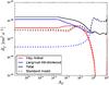 |
Fig. 13 H2 formation parameter Rf (full treatment: solid lines, standard treatment: dashed lines) for the two processes in a cloud with nH = 103 cm-3 and G0 = 10. |
For low radiation field models, the full treatment increases the LH mechanism at the edge to a level comparable or even higher than the ER mechanism, as shown in Fig. 13. The LH formation rate is increased by more than one order of magnitude and becomes higher than the ER rate, while it was one order of magnitude below in the standard rate equation model. The net result is an increase of the total formation rate by a factor of 4. While we were expecting the ER mechanism to be slightly decreased by the full treatment, we can note that it is slightly increased here. This is due to the gas temperature sensitivity of the ER mechanism. In this low radiation field model, the heating of the gas due to H2 formation is not negligible compared to the usually dominant photoelectric effect. A higher total H2 formation rate increases the heating of the gas resulting in a higher temperature at the edge (see Fig. 14). The ER mechanism is thus made slightly more efficient.
The main effect is a shift of the H / H2 transition from AV = 4 × 10⁻² to AV = 8 × 10⁻³, as shown of Fig. 15. As a result, the column density of excited H2 is increased, as shown in Table 4. As we are in low excitation conditions, the effect is mainly visible on the levels v = 0,J = 2 and v = 0,J = 3.
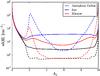 |
Fig. 17 Atomic H abundance in a cloud with nH = 104 cm-3 and G0 = 102. Comparison of rate equations results (dashed lines) with our full treatment (solid lines). |
We also note a significant increase of the H2 abundance before the transition, which results in increased CH+ formation at the edge. This effect and the higher temperature at the edge result in stronger excited lines of CH+ with differences of a factor of 2 on line (4−3). The excitation temperature computed from the observed intensities above (4−3) closely follow the change in gas temperature at the edge. The increase in intensity thus becomes larger as we go to larger levels, but those intensities remain most probably unobservable in this case.
The situation is different for high radiation field PDRs. The increase in the efficiency of the LH mechanism at the edge is not sufficient to make it comparable to the ER mechanism and the net result is a decrease of the total formation rate as the ER efficiency is reduced (see Fig. 16). This results in inverse effects with the H / H2 transition slightly shifted away from the edge, but of smaller amplitude as the formation rate difference is much smaller.
We present a wider investigation of the effects on observable intensities in Sect. 5.2, covering a large domain of cloud conditions.
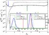 |
Fig. 19 Same cloud as Fig. 17, with formation parameter Rf for the LH mechanism, comparing standard (dashed black) and coupled (solid black) models. The insets show the effect of fluctuations on a 1 nm grain at the two positions in the cloud marked by the arrows. Blue: temperature PDF, red: equilibrium temperature, dashed green: equilibrium efficiency, and solid green: conditional efficiency with fluctuations. See the text for more details. |
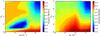 |
Fig. 20 H2 formation efficiency at the edge of the cloud as a function of the gas density nH and the radiation field intensity G0. The standard models (left) are compared with the full coupled models (right). |
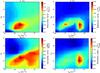 |
Fig. 21 Effect on H2 rotational lines intensities S(0) to S(3), shown as a comparison between the full computation result and the standard PDR result (neglecting dust temperature fluctuations). Parameters are the gas density nH and the scaling factor of the radiation field G0. |
5.1.2. Effects on cloud cores
Unexpectedly, temperature fluctuations of small dust grains are found to have an effect
on H2 formation
even in cloud cores where the UV field has been fully extinguished. As an example, Fig.
17 shows the atomic hydrogen abundance in a
specific cloud (nH = 104 cm-3,
χ = 100,
total AV = 10) and
compares the standard models to the coupled models with full treatment of the
fluctuations for the different binding energy values of Table 1. The residual atomic H abundance in the core is found to be systematically higher when
taking the fluctuations into account, which is a direct consequence of a lower formation
efficiency (the efficiencies are shown for the same models in Fig. 18). We recall that the formation efficiency is defined as the ratio
between the formation rate and half the collision rate between H atoms and grains (whose expression is
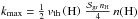 ), as this rate is the maximum formation
rate that would occur if one molecule was formed every two collisions. We also notice
that standard models tend to show a strong variability of the formation efficiency (and
consequently of the H
abundance) with a gap around AV = 2 with very low
efficiency, where neither the ER mechanism (the gas is not warm enough) nor the LH
mechanism (the grains are too warm) are efficient. This variability disappears in the
coupled models as fluctuations make the LH mechanism much less dependent on the grain
equilibrium temperature (see Sect. 4.2), and the
efficiency stays of the order of 10% (for amorphous carbon surfaces) across the cloud.
), as this rate is the maximum formation
rate that would occur if one molecule was formed every two collisions. We also notice
that standard models tend to show a strong variability of the formation efficiency (and
consequently of the H
abundance) with a gap around AV = 2 with very low
efficiency, where neither the ER mechanism (the gas is not warm enough) nor the LH
mechanism (the grains are too warm) are efficient. This variability disappears in the
coupled models as fluctuations make the LH mechanism much less dependent on the grain
equilibrium temperature (see Sect. 4.2), and the
efficiency stays of the order of 10% (for amorphous carbon surfaces) across the cloud.
The formation efficiency at the center of the cloud is decreased by almost one order of magnitude when including the fluctuations. This unexpected effect is detailed in Fig. 19 for amorphous carbon surfaces: the formation parameter Rf for the LH mechanism is shown for the standard model (black dashed line) and the coupled model (black solid line), and two inset plots show the effect of fluctuations on a 1 nm grain at two positions (AV = 0.5 and AV = 5, marked, respectively, by the blue and green vertical arrows on the main plot). Each inset contains a plot similar to Fig. 5, displaying the temperature PDF (blue line), the equilibrium temperature (red line), the equilibrium efficiency curve (dashed green line), and the effective conditional efficiency curve when taking fluctuations into account (solid green line).
Close to the edge of the cloud (at AV = 0.5), the situation is similar to the discussion of Fig. 5 (see Sect. 4.2). The main effect occurs because the temperature PDF has an important part inside the efficiency domain, while the equilibrium temperature is out of this domain. It results in increased efficiency. The dangers of using the equilibrium temperature are strikingly emphasized on this figure: when allowing fluctuations, a very small fraction of high temperature grains is sufficient to radiate away all the absorbed energy and most of the grains can be cold, while the grains must all be warm enough to balance the absorbed energy if we force them all to have a single temperature.
Deeper in the cloud (at AV = 5), the situation is different: the equilibrium temperature now falls close to the actual peak of the PDF and inside the efficiency domain, so that the actual position and spread of the PDF does not change the result much. The dominant effect is now that the conditional efficiency with fluctuations is strongly reduced compared to the equilibrium efficiency. As discussed in Sect. 4.2, this reduction comes from the competition between the fluctuation timescale and the adsorption timescale. At this optical depth, the grains are mainly heated by IR photons emitted by the hot dust at the edge, and for 1 nm grains, the IR photons are sufficient to bring the grains temporarily out of the efficiency domain (above 18 K here) where they lose their surface population. On the other hand, adsorption of H atoms are extremely rare, as the gas is almost completely molecular. As a result, the grain rarely manages to have two atoms on its surface, and the formation efficiency is thus reduced.
The effect described here concern very small grains, and one might question the presence of such very small grains and PAHs deep in the cloud core (the grain population is independent of position in our model). However, secondary UV photons, which were not considered for grain heating in these models, could induce a similar effect for much bigger grains, and further reduce the formation efficiency at high optical depth inside the cloud. This mechanism tends to increase the residual atomic H fraction in the core and could be relevant in explaining the slightly higher than expected atomic H abundances deduced from observations of HI self-absorption in dark clouds (e.g., Li & Goldsmith 2003).
No detectable effects on intensities were found in these models but the inclusion of secondary UV photons may induce stronger effects.
5.2. Grid of models
A grid of constant density PDR models was run to check the effect on observable intensities over a wider parameter range. We explore gas densities from nH = 102 cm-3 to nH = 3 × 105 cm-3 and scaling factors on the standard ISRF (Mathis et al. 1983) from 1 to 104 (as explained previously, the scaling factor only affects the UV part of the radiation field).
The effects of the fluctuations are mostly found on tracers of the PDR edges. The formation efficiency at the edge of the cloud is shown as a color map in Fig. 20, which compares the standard models with the full models including fluctuations. In the upper part of the map, the ER formation is decreased, and the LH mechanism remains negligible, resulting in an overall (small) decrease in efficiency. In the lower part, the LH mechanism is not negligible anymore, and its strong increase due to fluctuations results in an overall increase in efficiency. The region around G0 = 10 and nH = 103 − 104cm-3 is strikingly affected. In this region, the ER mechanism stops being efficient due to the low gas temperature at the edge. In standard models, the equilibrium temperature of the dust at the edge is still too high for the LH mechanism to work, giving a very low total formation efficiency. When taking into account fluctuations, the LH mechanism works efficiently, assuring a high formation efficiency. The effect is further amplified as gas heating by H2 formation is dominant in this region. The efficient LH formation heats up the gas, thus keeping ER formation efficient as well.
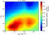 |
Fig. 22 Effect on H2 ro-vibrational line intensity (1−0) S(1), shown as a comparison between the full computation result and the standard PDR result (neglecting dust temperature fluctuations). Parameters are the gas density nH and the scaling factor of the radiation field G0. |
Figure 21 shows the modification of the H2 lower rotational intensities as the ratio between the result of the full computation, which includes dust temperature fluctuations, and the result of a standard PDR model. Higher rotational lines are affected very similarly to the S(3) line. Figure 22 shows the effect on the ro-vibrationnal line (1−0) S(1) in the same way. As expected from our discussion of Fig. 20, we see increased intensities for low radiation fields (roughly G0< 200), especially in regions where the gas temperature is highly sensitive on H2 formation heating and where LH formation can further trigger an amplification of ER formation. For higher radiation fields, the intensities are slightly decreased. The effect remains small, the increase for low radiation field models is at most a factor of 2.7 (on the S(1) line), and the decrease on the high radiation field models is at most 30%.
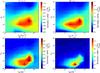 |
Fig. 23 Effect on CH+ line intensities, shown as a comparison between the full computation result and the standard PDR result (neglecting dust temperature fluctuations). Parameters are the gas density nH and the scaling factor of the radiation field G0. |
Another species affected by the more efficient formation of H2 at the edge is CH+. It is formed by the reaction of C+ + H2, which is allowed by the high gas temperature at the edge of the PDR and by the internal energy of the H2 molecule, as described in Agúndez et al. (2010) (pumped by UV photons and by its formation process). A higher H2 formation rate at the edge induces a higher H2 fraction before the transition, which leads to a higher CH+ formation rate. Gas heating by H2 formation can further enhance its formation. Figure 23 shows the effect on CH+ intensities. We again observe increased emission in the domain where the H2 formation efficiency is enhanced, due to both higher abundances of CH+ and higher gas temperatures. The domain of strong enhancement is quite similar to the one for H2 rotational lines, corresponding to the domain where gas heating is dominated by H2 formation heating. This temperature effect is visible on all high excitation lines emitted before the H / H2 transition (e.g., the most excited lines of HCO+, CS, HCN, ...).
6. Conclusion and perspectives
We presented a method to compute H2 formation on dust grains taking fully the fluctuating temperature of the grain for both the ER and the LH mechanism into account.
As a side result of this work, we revisited the computation of dust temperature fluctuations. We confirm that the continuous cooling approximation (e.g., used in DustEM) is sufficient for an accurate computation of the mid- and near-infrared spectrum. However, the detailed treatment of surface processes requires a better estimation of the low temperature part of the dust temperature PDF, which is done in this paper by including the discrete nature of photon emission.
The coupled fluctuations problem was solved exactly for both the ER and the LH mechanisms. A numerically efficient way of computing the ER formation rate was found. The effect on the ER formation rate is limited to a factor of 2, and the effect on full cloud simulations is limited. The standard rate equation treatment of this ER mechanism is thus a good treatment for the purpose of complete PDR simulations.
With the exact solution for the LH mechanism being numerically intractable for big grains, we constructed an approximation based on simple physical arguments to compute the fluctuation effect on the LH mechanism and checked for small grains that the approximation yields accurate results. The effect is strong as fluctuating grains spend a significant part of their time in the low temperature range, in which formation is efficient, even when their average temperature is out of the rate equation efficiency domain. This results in a strong increase in LH formation efficiency in unshielded environments where the average dust temperature is high and only fluctuations can allow LH formation.
The LH mechanism is found to become of comparable importance with the ER mechanism at the edge of PDRs, except for strong radiation fields. The resulting increase of H2 formation rate at the edge induces a shift in the H / H2 transition toward the edge of the PDR. The resulting effect on observable lines emitted in this region remains limited and does not reach one order of magnitude in the strongest cases.
On the contrary, fluctuations of the smallest grains caused by IR photons reduce the formation efficiency by almost one order of magnitude in the core of the clouds, as collisions with H atoms in a completely molecular gas are much rarer than absorption of IR photons heating temporarily the grain above 18 K. No significant effects are found on intensities, but including secondary UV photons could induce stronger effects.
Overall, the variations induced in observational intensities are comparable to what can be expected from many other poorly known parameters. The interpretation of observations with standard PDR codes, thus, need not use the detailed treatment analyzed here and a simple rate coefficient approximation can be used most of the time. However, this cannot be blindly extended to any arbitrary process and must be checked in each specific case. In particular, the existence of temperature fluctuations of the smallest grains deep inside the cloud should be taken into account for other surface chemical processes. Possible consequences on the abundance of light organic molecules are currently being investigated.
We neglect energy discretization for the lower states, and adopt the normalization E = 0 for T = 0. See Li & Draine (2001) for a detailed state-by-state treatment.
Acknowledgments
This work was funded by grant ANR-09-BLAN-0231-01 from the French Agence Nationale de la Recherche as part of the SCHISM project. We thank Laurent Verstraete for fruitful discussions on dust properties, and Evelyne Roueff for many discussions. We thank our referee for his useful comments.
References
- Agúndez, M., Goicoechea, J. R., Cernicharo, J., Faure, A., & Roueff, E. 2010, ApJ, 713, 662 [NASA ADS] [CrossRef] [Google Scholar]
- Bachellerie, D., Sizun, M., Aguillon, F., et al. 2009, Phys. Chem. Chem. Phys., 11, 2715 [CrossRef] [PubMed] [Google Scholar]
- Biham, O., & Lipshtat, A. 2002, Phys. Rev. E, 66, 056103 [NASA ADS] [CrossRef] [Google Scholar]
- Bonfanti, M., Casolo, S., Tantardini, G. F., Ponti, A., & Martinazzo, R. 2011, J. Chem. Phys., 135, 164701 [NASA ADS] [CrossRef] [Google Scholar]
- Casolo, S., Løvvik, O. M., Martinazzo, R., & Tantardini, G. F. 2009, J. Chem. Phys., 130, 054704 [NASA ADS] [CrossRef] [PubMed] [Google Scholar]
- Casolo, S., Tantardini, G. F., & Martinazzo, R. 2013, Proc. Nat. Acad. Sci., 110, 6674 [NASA ADS] [CrossRef] [Google Scholar]
- Cazaux, S., & Tielens, A. G. G. M. 2004, ApJ, 604, 222 [NASA ADS] [CrossRef] [Google Scholar]
- Chang, Q., Cuppen, H. M., & Herbst, E. 2005, A&A, 434, 599 [NASA ADS] [CrossRef] [EDP Sciences] [Google Scholar]
- Chang, Q., Cuppen, H. M., & Herbst, E. 2006, A&A, 458, 497 [NASA ADS] [CrossRef] [EDP Sciences] [Google Scholar]
- Combes, F., & Pineau des Forets, G., 2001, Molecular Hydrogen in Space (Cambridge, UK: Cambridge University Press) [Google Scholar]
- Compiègne, M., Verstraete, L., Jones, A., et al. 2011, A&A, 525, A103 [NASA ADS] [CrossRef] [EDP Sciences] [Google Scholar]
- Cuppen, H. M., & Herbst, E. 2005, MNRAS, 361, 565 [NASA ADS] [CrossRef] [Google Scholar]
- Cuppen, H. M., Morata, O., & Herbst, E. 2006, MNRAS, 367, 1757 [NASA ADS] [CrossRef] [Google Scholar]
- Desert, F. X., Boulanger, F., & Shore, S. N. 1986, A&A, 160, 295 [NASA ADS] [Google Scholar]
- Draine, B. T., & Li, A. 2001, ApJ, 551, 807 [NASA ADS] [CrossRef] [Google Scholar]
- Du, Y. 2006, Order Structure and Topological Methods In Nonlinear partial Differential Equations., Vol. 1: Maximum Principles and Applications (World Scientific) [Google Scholar]
- Duley, W. W. 1996, MNRAS, 279, 591 [NASA ADS] [CrossRef] [Google Scholar]
- Garrod, R. T. 2008, A&A, 491, 239 [NASA ADS] [CrossRef] [EDP Sciences] [Google Scholar]
- Gould, R. J., & Salpeter, E. E. 1963, ApJ, 138, 393 [NASA ADS] [CrossRef] [Google Scholar]
- Habart, E., Boulanger, F., Verstraete, L., Walmsley, C. M., & Pineau des Forêts, G. 2004, A&A, 414, 531 [NASA ADS] [CrossRef] [EDP Sciences] [Google Scholar]
- Habart, E., Abergel, A., Boulanger, F., et al. 2011, A&A, 527, A122 [NASA ADS] [CrossRef] [EDP Sciences] [Google Scholar]
- Hasegawa, T. I., Herbst, E., & Leung, C. M. 1992, ApJS, 82, 167 [NASA ADS] [CrossRef] [Google Scholar]
- Hollenbach, D., & Salpeter, E. E. 1971, ApJ, 163, 155 [NASA ADS] [CrossRef] [Google Scholar]
- Iqbal, W., Acharyya, K., & Herbst, E. 2012, ApJ, 751, 58 [NASA ADS] [CrossRef] [Google Scholar]
- Iqbal, W., Acharyya, K., & Herbst, E. 2014, ApJ, 784, 139 [NASA ADS] [CrossRef] [Google Scholar]
- Ivanovskaya, V. V., Zobelli, A., Teillet-Billy, D., et al. 2010, Phys. Rev. B, 82, 245407 [NASA ADS] [CrossRef] [Google Scholar]
- Jeloaica, L., & Sidis, V. 1999, Chem. Phys. Lett., 300, 157 [NASA ADS] [CrossRef] [Google Scholar]
- Katz, N., Furman, I., Biham, O., Pirronello, V., & Vidali, G. 1999, ApJ, 522, 305 [NASA ADS] [CrossRef] [Google Scholar]
- Kerwin, J., & Jackson, B. 2008, J. Chem. Phys., 128, 084702 [NASA ADS] [CrossRef] [Google Scholar]
- Le Bourlot, J., Le Petit, F., Pinto, C., Roueff, E., & Roy, F. 2012, A&A, 541, A76 [NASA ADS] [CrossRef] [EDP Sciences] [Google Scholar]
- Le Petit, F., Nehmé, C., Le Bourlot, J., & Roueff, E. 2006, ApJS, 164, 506 [NASA ADS] [CrossRef] [EDP Sciences] [Google Scholar]
- Le Petit, F., Barzel, B., Biham, O., Roueff, E., & Le Bourlot, J. 2009, A&A, 505, 1153 [NASA ADS] [CrossRef] [EDP Sciences] [Google Scholar]
- Lehtinen, P. O., Foster, A. S., Ma, Y., Krasheninnikov, A. V., & Nieminen, R. M. 2004, Phys. Rev. Lett., 93, 187202 [NASA ADS] [CrossRef] [PubMed] [Google Scholar]
- Li, A., & Draine, B. T. 2001, ApJ, 554, 778 [Google Scholar]
- Li, D., & Goldsmith, P. F. 2003, ApJ, 585, 823 [NASA ADS] [CrossRef] [Google Scholar]
- Lipshtat, A., & Biham, O. 2003, A&A, 400, 585 [NASA ADS] [CrossRef] [EDP Sciences] [Google Scholar]
- Lohmar, I., & Krug, J. 2006, MNRAS, 370, 1025 [NASA ADS] [CrossRef] [Google Scholar]
- Lohmar, I., Krug, J., & Biham, O. 2009, A&A, 504, L5 [NASA ADS] [CrossRef] [EDP Sciences] [Google Scholar]
- Martinazzo, R., & Tantardini, G. F. 2006, J. Chem. Phys., 124, 124703 [NASA ADS] [CrossRef] [Google Scholar]
- Mathis, J. S., Rumpl, W., & Nordsieck, K. H. 1977, ApJ, 217, 425 [NASA ADS] [CrossRef] [Google Scholar]
- Mathis, J. S., Mezger, P. G., & Panagia, N. 1983, A&A, 128, 212 [NASA ADS] [Google Scholar]
- Mennella, V. 2008, ApJ, 684, L25 [NASA ADS] [CrossRef] [Google Scholar]
- Morisset, S., Aguillon, F., Sizun, M., & Sidis, V. 2004a, J. Chem. Phys., 121, 6493 [NASA ADS] [CrossRef] [Google Scholar]
- Morisset, S., Aguillon, F., Sizun, M., & Sidis, V. 2004b, J. Phys. Chem. A, 108, 8571 [Google Scholar]
- Morisset, S., Aguillon, F., Sizun, M., & Sidis, V. 2005, J. Chem. Phys., 122, 194702 [NASA ADS] [CrossRef] [Google Scholar]
- Perets, H. B., Lederhendler, A., Biham, O., et al. 2007, ApJ, 661, L163 [NASA ADS] [CrossRef] [Google Scholar]
- Pirronello, V., Liu, C., Roser, J. E., & Vidali, G. 1999, A&A, 344, 681 [NASA ADS] [Google Scholar]
- Pirronello, V., Biham, O., Liu, C., Shen, L., & Vidali, G. 1997a, ApJ, 483, L131 [NASA ADS] [CrossRef] [Google Scholar]
- Pirronello, V., Liu, C., Shen, L., & Vidali, G. 1997b, ApJ, 475, L69 [NASA ADS] [CrossRef] [Google Scholar]
- Rougeau, N., Teillet-Billy, D., & Sidis, V. 2011, Phys. Chem. Chem. Phys., 13, 17579 [CrossRef] [Google Scholar]
- Sha, X., & Jackson, B. 2002, Surface Science, 496, 318 [NASA ADS] [CrossRef] [Google Scholar]
- Sizun, M., Bachellerie, D., Aguillon, F., & Sidis, V. 2010, Chem. Phys. Lett., 498, 32 [NASA ADS] [CrossRef] [Google Scholar]
- Sternberg, A., & Dalgarno, A. 1995, ApJS, 99, 565 [NASA ADS] [CrossRef] [Google Scholar]
Appendix A: Effect of H2 formation energy on the equilibrium rate equation calculation
We first consider the heating of the grain by the Eley-Rideal mechanism. Each formation reaction gives 1 eV to the grain.
The liberation of energy left in the grain by each formation reaction creates an additional coupling between the surface population and the grain temperature. The method described in Sect. 2.2.2, which was based on a one-way coupling between the two variables, is thus not possible here.
To evaluate this effect, we use the standard equilibrium temperature equation and chemical rate equation with a coupling term representing the heating of the grain by the formation reaction. We assume that each formation reaction gives an energy EfH2 = 1 eV to the grain, which is instantly converted into thermal energy.
For ER formation on chemisorption sites, we thus have the system of equations:
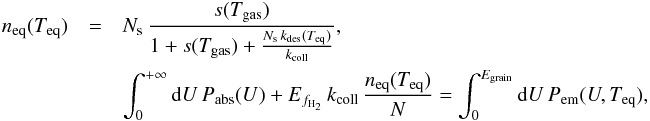 which can be easily solved. However, we find
that the effect of this average heating of the grain by formation reactions is completely
negligible in the range of realistic values of parameters, resulting in a change of the
grain temperature by less than 1%.
which can be easily solved. However, we find
that the effect of this average heating of the grain by formation reactions is completely
negligible in the range of realistic values of parameters, resulting in a change of the
grain temperature by less than 1%.
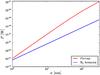 |
Fig. A.1 Heating power received by a grain as a function of grain size. Power received from photons in red and H2 formation in blue. |
Independently of the detail of the formation mechanism, we can put an upper limit on the
heating term caused by H2 formation by assuming that all H atoms hitting the grain are turned into
H2. In this case,
the formation rate is simply  , and the heating power is
 . We can then compare this term to the
absorbed power coming from photons.
. We can then compare this term to the
absorbed power coming from photons.
The result is shown here in Fig. A.1 in an extreme case with a low radiation field (G0 = 1) and a high collision rate (atomic gas with n = 103 cm-3 and T = 350 K). Despite assuming a total formation efficiency in a low radiation field, high collision rate environment, we can see that the heating term due to H2 formation becomes barely significant only for the smallest grain sizes. We can thus safely neglect the grain heating coming from H2 formation (through the ER mechanism, and all the more for the LH mechanism as the EfH2 is probably much lower as physisorbed atoms are much more weakly bound) in most usual conditions. Moreover, under a radiation field with G0 = 1, the gas would not be as warm as we assumed here and the ER efficiency would be very low.
Appendix B: Eigenvalues of the integral operator for the thermal energy PDF
The operator ℒ defined in
equation 8 can be rewritten as
=\int_{0}^{+\infty}{\rm{d}}E'\, A(E,E')\, f(E') \end{eqnarray*}](/articles/aa/full_html/2014/09/aa22101-13/aa22101-13-eq295.png) with
with ![Mathematical equation: \appendix \setcounter{section}{2} \begin{eqnarray*} A(E,E')=\begin{cases} {\displaystyle \frac{R_{\mathrm{abs}}(E-E')}{P(E)}} & \mathrm{if}\quad E'<E\\[2.5mm] {\displaystyle \frac{R_{\mathrm{em}}(E'-E,T(E'))}{P(E)}} & \mathrm{if}\quad E'\ge E, \end{cases} \end{eqnarray*}](/articles/aa/full_html/2014/09/aa22101-13/aa22101-13-eq296.png) where
where 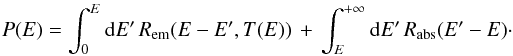 The existence of a solution to our problem is
equivalent to the existence of a positive eigenfunction associated with the eigenvalue 1.
The existence of a solution to our problem is
equivalent to the existence of a positive eigenfunction associated with the eigenvalue 1.
This operator is continuous, compact, and strongly positive. The Krein-Rutman theorem (see Du 2006, Chap. 1) tells us that its spectral radius is a simple eigenvalue associated with a positive eigenfunction and that this eigenfunction is the only positive eigenfunction.
We first show that 1 is an eigenvalue of the adjoint operator
=\int_{0}^{+\infty}{\rm{d}}E'\, A(E',E)\, f(E')$}](/articles/aa/full_html/2014/09/aa22101-13/aa22101-13-eq298.png) and that it is associated with a positive
eigenfunction. We can easily find such a positive eigenfunction with the eigenvalue 1 for
this adjoint operator:
and that it is associated with a positive
eigenfunction. We can easily find such a positive eigenfunction with the eigenvalue 1 for
this adjoint operator: } & = & {\displaystyle \int_{0}^{+\infty}{\rm{d}}E'\, A(E',E)\, P(E')} \\[1.5mm] \, & = & {\displaystyle {\displaystyle \int_{0}^{E}{\rm{d}}E'\frac{R_{\mathrm{em}}(E-E',T(E))}{P(E')}P(E')}}\\ \, & + & {\displaystyle {\displaystyle \int_{E}^{+\infty}{\rm{d}}E'\frac{R_{\mathrm{abs}}(E'-E)}{P(E')}P(E')}}\\ \, & = & {\displaystyle P(E)}, \end{eqnarray*}](/articles/aa/full_html/2014/09/aa22101-13/aa22101-13-eq299.png) and P(E) is a positive function. Thus, 1 is
the spectral radius of ℒ∗ and hence of ℒ. This proves the existence and the unicity of the solution to our
problem. Moreover, it proves that all the other eigenvalues λ are such that
| λ | ≤ 1
and thus Re(λ) < 1. We can therefore
iterate the application of the operator to an initial function and converge toward the
solution, assuming that the initial function is not orthogonal to the solution. Starting
with a positive initial function is sufficient.
and P(E) is a positive function. Thus, 1 is
the spectral radius of ℒ∗ and hence of ℒ. This proves the existence and the unicity of the solution to our
problem. Moreover, it proves that all the other eigenvalues λ are such that
| λ | ≤ 1
and thus Re(λ) < 1. We can therefore
iterate the application of the operator to an initial function and converge toward the
solution, assuming that the initial function is not orthogonal to the solution. Starting
with a positive initial function is sufficient.
Appendix C: Verification of the approximations
In this appendix, we evaluate the accuracy of our approximations by comparing their results to those of the exact methods presented in Sect. 2.2.
Appendix C.1: LH mechanism
For the LH mechanism, the exact method (cf. Sect. 2.2.3) is only tractable for a limited range of grain sizes. We compare the approximation (cf. Sect. 3.1) with it on this range and verify that the approximation joins the equilibrium result for bigger grains.
 |
Fig. C.1 Approximated ⟨n|T⟩ (dashed lines) for the LH mechanism compared to the exact results (solid lines). Model with gas density n = 103 cm-3 and G0 = 20 with barrier and binding energies for ices. For clarity, each successive curve has been shifted by a factor of ten. |
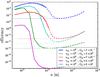 |
Fig. C.2 Approximated LH formation efficiency for one grain (dashed lines) compared to the exact results (solid lines). The formation efficiencies at the constant equilibrium temperatures are shown in dotted lines. The densities are given in cm-3. The binding and barrier energies correspond to ices. |
Figure C.1 shows the resulting curves for ⟨n|T⟩ for different grain sizes and compares the approximation to the exact result. The binding and barrier energies are taken for ice surfaces in Table 1. We see a very good match for small grains in the low temperature domain. Large discrepancies appear at high temperature but do not matter for the average formation rate on the grain as the contribution of this regime is negligible. For bigger grains, the approximation of the low temperature regime starts to be less accurate. However, we know that total formation rate is mostly influenced by the smallest grain sizes due to the −3.5 exponent of the size distribution.
Approximation error on the final formation rate integrated over the full size distribution for the LH mechanism.
The resulting formation rate per grain is shown in Fig. C.2 as a function of grain size for 5 models spanning the parameter domain. We again assumed here an ice surface. The match is very good on the domain on which the exact computation could be performed, and the approximation smoothly joins with the equilibrium result neglecting fluctuations for big grains. The relative errors on the final formation rate integrated over the size distribution are given for each model in the first part of Table C.1. The results are given for two size distributions. Both are MRN-like power-law distributions with exponent −3.5, but one starts at 5 Å and the other at 1 nm. Both go up to 0.3 μm. We find extremely accurate results for the approximation in most case with a relative error at most around 5%.
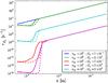 |
Fig. C.4 Approximated ER formation rate for one grain (dashed lines) compared to the exact results (solid lines). The densities are given in cm-3. |
When using the energy values corresponding to an amorphous carbon surface (see Table 1), the same levels of accuracy are achieved. The formation rate as a function of grain size is shown in Fig. C.3. When integrated over the size distribution, the formation rate obtained from the approximation is again within 5% from exact result (see second part of Table C.1).
Approximation error on the final formation rate integrated over the full size distribution for the ER mechanism.
Appendix C.2: ER mechanism
We now perform the same verification for the ER mechanism. The approximation of Sect. 3.2 is compared to the exact method of Sect. 2.2.2. Figure C.4 shows the formation rate as a function of grain size. The qualitative effect is captured by the approximation, but large discrepancies appear locally for some sizes, due to a shifted transition from a low efficiency regime to a high efficiency one. However, the results when integrating over the dust size distribution remain reasonably accurate, as shown in Table C.2. We recall that this approximation is not used in this paper as the exact method is numerically efficient.
All Tables
Approximation error on the final formation rate integrated over the full size distribution for the LH mechanism.
Approximation error on the final formation rate integrated over the full size distribution for the ER mechanism.
All Figures
|
Fig. 1 Dust thermal energy PDFs for three grain sizes (amorphous carbon grains under a radiation field with G0 = 120). |
| In the text | |
|
Fig. 2 Equilibrium temperature (dashed line) and actual average temperature (solid line), as a function of the grain size for the three types of grains (radiation field G0 = 120). |
| In the text | |
|
Fig. 3 Local dust emissivity (emitted power per unit of volume) as a function of wavelength for a dust population corresponding to Compiègne et al. (2011) under a radiation field with G0 = 100. We compare our code, Fredholm, with DustEM. |
| In the text | |
|
Fig. 4 Formation efficiency (LH mechanism) on one grain (carbonaceous) as a function of size for different radiation field intensities (in a gas at nH = 104 cm-3, T = 100 K). Solid lines: full computation. Dashed line: equilibrium rate equation results. The binding and barrier energies correspond to ices. |
| In the text | |
|
Fig. 5 Temperature PDF (blue line, left axis) for a 3 nm carbonaceous dust grain, as compared to the formation efficiency (LH mechanism) as a function of temperature (green lines, right axis). The red vertical line marks the mean temperature of the blue PDF. The grain receives a G0 = 20 radiation field and is surrounded by a 100 K gas with nH = 104 cm-3. The energy values correspond to ices. |
| In the text | |
|
Fig. 6 Integrated formation rate parameter Rf (LH mechanism) for a carbonaceous dust population (see Table 3) as a function of the radiation field intensity G0 for different gas densities (the gas temperature is fixed at 100 K). Solid lines: full computation. Dashed lines: equilibrium rate equation results. Binding and barrier energies corresponding to ices. |
| In the text | |
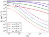 |
Fig. 7 Same as Fig. 6 with binding and barrier energies corresponding to amorphous carbon surfaces. |
| In the text | |
|
Fig. 8 Conditional mean of the surface coverage (chemisorption only) as a function of grain temperature for three sizes of amorphous carbon grains (solid lines) and equilibrium coverage (dashed line). The grain is surrounded by gas at density nH = 104 cm-3 and temperature T = 350 K under a radiation field with G0 = 120. |
| In the text | |
|
Fig. 9 H2 formation efficiency (ER mechanism) as a function of grain size for various radiation fields (carbonaceous grains in a gas at nH = 104 cm-3 and T = 350 K). |
| In the text | |
|
Fig. 10 Integrated formation rate Rf (ER mechanism) over a full dust size distribution (see Table 3) as a fraction of the equilibrium rate equation result. The result is shown for three different gas densities (thus changing the collision rate) as a function of the radiation field intensity. |
| In the text | |
|
Fig. 11 Integrated formation rate ratio (ER mechanism) over a full dust size distribution, as a function of the radiation field intensity when changing the inferior limit of the grain size distribution (nH = 104 cm-3). |
| In the text | |
|
Fig. 12 Integrated formation rate ratio (ER mechanism) over a full dust size distribution, as a function of the radiation field intensity for different chemisorption binding energies (nH = 104 cm-3). |
| In the text | |
|
Fig. 13 H2 formation parameter Rf (full treatment: solid lines, standard treatment: dashed lines) for the two processes in a cloud with nH = 103 cm-3 and G0 = 10. |
| In the text | |
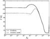 |
Fig. 14 Gas temperature (same cloud as Fig. 13). |
| In the text | |
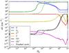 |
Fig. 15 Abundances of the species of interest in the same cloud as Fig. 13. |
| In the text | |
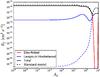 |
Fig. 16 Same as Fig. 13 for a cloud with nH = 103 cm-3 and G0 = 103. |
| In the text | |
|
Fig. 17 Atomic H abundance in a cloud with nH = 104 cm-3 and G0 = 102. Comparison of rate equations results (dashed lines) with our full treatment (solid lines). |
| In the text | |
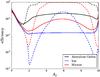 |
Fig. 18 H2 formation efficiency. Same case as Fig. 17. |
| In the text | |
|
Fig. 19 Same cloud as Fig. 17, with formation parameter Rf for the LH mechanism, comparing standard (dashed black) and coupled (solid black) models. The insets show the effect of fluctuations on a 1 nm grain at the two positions in the cloud marked by the arrows. Blue: temperature PDF, red: equilibrium temperature, dashed green: equilibrium efficiency, and solid green: conditional efficiency with fluctuations. See the text for more details. |
| In the text | |
|
Fig. 20 H2 formation efficiency at the edge of the cloud as a function of the gas density nH and the radiation field intensity G0. The standard models (left) are compared with the full coupled models (right). |
| In the text | |
|
Fig. 21 Effect on H2 rotational lines intensities S(0) to S(3), shown as a comparison between the full computation result and the standard PDR result (neglecting dust temperature fluctuations). Parameters are the gas density nH and the scaling factor of the radiation field G0. |
| In the text | |
|
Fig. 22 Effect on H2 ro-vibrational line intensity (1−0) S(1), shown as a comparison between the full computation result and the standard PDR result (neglecting dust temperature fluctuations). Parameters are the gas density nH and the scaling factor of the radiation field G0. |
| In the text | |
|
Fig. 23 Effect on CH+ line intensities, shown as a comparison between the full computation result and the standard PDR result (neglecting dust temperature fluctuations). Parameters are the gas density nH and the scaling factor of the radiation field G0. |
| In the text | |
|
Fig. A.1 Heating power received by a grain as a function of grain size. Power received from photons in red and H2 formation in blue. |
| In the text | |
|
Fig. C.1 Approximated ⟨n|T⟩ (dashed lines) for the LH mechanism compared to the exact results (solid lines). Model with gas density n = 103 cm-3 and G0 = 20 with barrier and binding energies for ices. For clarity, each successive curve has been shifted by a factor of ten. |
| In the text | |
|
Fig. C.2 Approximated LH formation efficiency for one grain (dashed lines) compared to the exact results (solid lines). The formation efficiencies at the constant equilibrium temperatures are shown in dotted lines. The densities are given in cm-3. The binding and barrier energies correspond to ices. |
| In the text | |
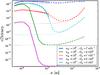 |
Fig. C.3 Same as Fig. C.2 for binding and barrier energies corresponding to amorphous carbon grains. |
| In the text | |
|
Fig. C.4 Approximated ER formation rate for one grain (dashed lines) compared to the exact results (solid lines). The densities are given in cm-3. |
| In the text | |
Current usage metrics show cumulative count of Article Views (full-text article views including HTML views, PDF and ePub downloads, according to the available data) and Abstracts Views on Vision4Press platform.
Data correspond to usage on the plateform after 2015. The current usage metrics is available 48-96 hours after online publication and is updated daily on week days.
Initial download of the metrics may take a while.