| Issue |
A&A
Volume 568, August 2014
|
|
|---|---|---|
| Article Number | A44 | |
| Number of page(s) | 10 | |
| Section | Astronomical instrumentation | |
| DOI | https://doi.org/10.1051/0004-6361/201323299 | |
| Published online | 11 August 2014 | |
Observations of optically active turbulence in the planetary boundary layer by sodar at the Concordia astronomical observatory, Dome C, Antarctica
1 Institute of Atmospheric Sciences and Climate, ISAC/CNR, via del Fosso del Cavaliere 100, 00133 Roma, Italy
e-mail: This email address is being protected from spambots. You need JavaScript enabled to view it.
2 Laboratoire Lagrange, UMR 7293 UNS/CNRS/OCA, University of Nice, Parc Valrose, 06108 Nice Cedex, France
3 A.M.Obukhov Institute of Atmospheric Physics/RAS, Pyzhevsky per., 3, 119017 Moscow, Russia
4 GEMAC, University of Versailles/CNRS, 45 av. des Etats-Unis, 78035 Versailles Cedex, France
5 Le Mée-sur-Seine, France
Received: 20 December 2013
Accepted: 19 May 2014
Abstract
Aims. An experiment was set up at the Concordia station in Antarctica during the winter-over period in 2012 to determine the behaviour of atmospheric optical turbulence in the lower part of the atmospheric boundary layer. The aim of the experiment was to study the influence of turbulence and weather conditions on the quality of astronomical observations. The Concordia station is characterised by the high quality of astronomical images thanks to very low seeing values. The surface layer in the interior of Antarctica during the winter is very stably stratified with the differences of temperature between the surface and the top of the inversion, which reach 20−35°C. In spite of this strong static stability, considerable thermal optically active turbulence sometimes occurs and extends to several tens of metres above the surface, depending on weather conditions. It is important to know the meteorological characteristics that favour good astronomical observations.
Methods. The optical measurements of the seeing made by differential image motion monitors installed at two levels of 8 and 20 m were accompanied by observations of turbulence in the lowest one hundred meters. Turbulence was detected and evaluated using a high-resolution sodar developed specially for this purpose. The statistics of some relevant meteorological variables including the long-wave downward radiation, which indicates cloudiness, were determined.
Results. Typical patterns of the vertical and temporal structure of turbulence shown by sodar echograms were identified, analysed, and classified. The statistics of the depth of the surface-based turbulent layer and the turbulent optical factor for different height layers are presented together with the seeing statistics. We analysed the dependence of both seeing and integral turbulence intensity within the first 100 m on temperature and wind speed.
Conclusions. Seeing and turbulence intensity in the atmospheric boundary layer appear to be correlated. The best values of the seeing (<1 arcsec) are observed when the sodar shows very low turbulence intensity. The main contribution to the image distortion is due to turbulence generated within the lowest 30−50 m near the surface. The presented statistics of the vertical distribution of the atmospheric optical turbulence can be used to determine the optimal location for astronomical instruments.
Key words: turbulence / site testing / atmospheric effects
© ESO, 2014
1. Introduction
One of the main factors that significantly affect the quality of astronomical observations is the atmospheric turbulence; it causes blurred images. The effect of turbulence on the quality of astronomical images is described by a parameter called seeing. The seeing, β, can be characterised by the full width at half maximum of the long-exposure atmospheric point spread function at a wavelength of 500 nm. Typical values of the seeing in good astronomical sites are around 0.7 arcsec, “bad” seeing is above 1.5 arcsec (Aristidi et al. 2005a). Studying the distorting action of the atmospheric turbulence is important to understand the reasons of the seeing variability, which in turn is necessary to be able to reliably predict the quality of the astronomical observations.
The intensity of optically active turbulence at an altitude h is described by the refraction index structure parameter (also called structural characteristic of the refraction index)  . The intensity of the turbulent temperature fluctuations is characterised by the temperature structure parameter
  . These different quantities can be compared thanks to the well established theory of wave propagation in turbulent media (Tatarskii 1971). These parameters are connected by the relationship
 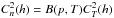 , with B(p,T) = (79.2 × 10⁻⁶pT-2)2, where p is the air pressure in mbar, T is the absolute temperature in K, and the numerical coefficient is appropriated for the wavelength λ = 500 nm. The turbulent optical factor (TOF)
 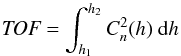 (1)evaluates the degree of degradation of a stellar image by Kolmogorov’s turbulence, which localised in the atmospheric layer between altitudes h1 and h2.
The practical application of the acoustic sounding method for systematic observations of the intensity of optically active turbulence in the atmospheric boundary layer (ABL) was realised by Gur’yanov et al. (1988) and Gur’yanov et al. (1992). The combined experiments were carried out at three mountain astronomical observatories of the former USSR to explain the difference in the quality of astronomical images at different sites. Vertical profiles of were measured with a calibrated sodar and a differential fluctuation thermometer. The seeing values β were determined from the optical measurements of the scintillation of a star image with a photoelectric seeing monitor. The magnitude of the turbulent optical factor over the entire depth of the atmosphere was estimated from the formula ![Mathematical equation: \begin{equation} \textit{TOF}_{\infty} = 6.9 \times 10^{-13} \beta^{\frac{5}{3}} \ \ \left[\mbox{m}^{\frac{1}{3}}\right], \end{equation}](/articles/aa/full_html/2014/08/aa23299-13/aa23299-13-eq14.png) (2)which was derived using the results by Tatarskii (1971) and Martin (1987). The contribution of the atmospheric turbulence in the lowest layer of a few hundred metres thickness to the distortion of astronomical images was evaluated to be small in those papers. The upper atmospheric layers were determined to be mainly responsible for the seeing.
(2)which was derived using the results by Tatarskii (1971) and Martin (1987). The contribution of the atmospheric turbulence in the lowest layer of a few hundred metres thickness to the distortion of astronomical images was evaluated to be small in those papers. The upper atmospheric layers were determined to be mainly responsible for the seeing.
The Dome C site is known as a place with excellent quality of astronomical images. Summer site-testing results based on differential image motion monitor (DIMM) measurements carried out at the Concordia station were presented by Aristidi et al. (2003) and Aristidi et al. (2005a). These data were collected on the bright star Canopus during two three-months summer campaigns (November–January) in 2003−2004 and 2004−2005. Seeing and isoplanatic angle in the visible were continuously monitored. The median seeing was found to be of 0.54 arcsec. The seeing appears to have a deep minimum around 0.4 arcsec almost every day in late afternoon. The statistics of the seeing at this observatory for the summer period (with a median of β = 0.54 arcsec and a percentage of excellent seeing β< 0.6 arcsec of 59%) is significantly better than at many other investigated sites.
The first winter (February–October) site-testing at this place was carried out in 2004 in automatic regime (Lawrence et al. 2004) using a remote autonomous laboratory equipped with a multi-aperture scintillation sensor (MASS) and a sodar. Further winter site-testing was carried out during the winter-over campaign performed in 2005. Its results based on balloon in-situ measurements of  with microthermal sensors and DIMM data obtained at the Concordia station were presented by Agabi et al. (2006), and later by Trinquet et al. (2008) and Aristidi et al. (2009). The sodar measurements carried out in 2004 (Lawrence et al. 2004) and 2005 (Argentini & Pietroni 2010) showed very weak atmospheric turbulence in the boundary layer above 30−50 m, but were not able to detect the turbulence behaviour within the lowest 30−50 m because of the technical limitations.
During the winter-over campaign of 2012 at the Concordia station, the method of acoustic sounding, with which the behaviour of the intensity of optical inhomogeneities can be determined, was used for regular long-time observations. The thermal turbulence in the PBL was measured by a high-resolution sodar that was specifically developed for this purpose and can probe the atmosphere from an altitude of ≈2 m with a vertical resolution of <2 m. The integrated effect of the entire atmosphere above was measured by two optical seeing monitors DIMM installed at two heights, 8 and 20 m. Section 2 describes the instrumentation set and site characteristics. In Sect. 3, we consider the results concerning for 1) some aspects of the meteorological conditions during the observational periods; 2) qualitative characteristics of thermal turbulence in the surface layer depicted by sodar; 3) statistical characteristics of the seeing; 4) correlation between sodar and optical estimates of the image quality; and 5) the height estimate of the atmospheric layer that provides the main contribution to distortion in astronomical images. Section 4 summarises the obtained results and provides some recommendations for the installation of astronomical instruments.
2. Site, instrumentation, measurements
2.1. Site location and characterisation
The Concordia station is located at Dome Charlie (Dome C), Antarctic plateau, East Antarctica, 1000 km inland from the nearest coast (75°06′S, 123°21′E, 3233 m a. s. l. ). The surface slope at this site is ≈0.1%. The Sun culminates at 38° on the 21 December and is permanently below the horizon from May, 6 to August, 9.
The local climate is dominated by strong temperature inversion (up to 35°C difference between near-surface and the top of the inversion layer) and weak katabatic winds blowing from the south-southwest sector under cold, clear, and calm weather conditions with temperatures reaching −80°C. Episodic synoptic perturbations due to the maritime (coastal) air intrusions are characterised by stronger wind speeds up to 12 m s , significantly higher temperatures (up to −40°C) and dense cloudiness (e.g. Argentini et al. 2001, Genthon et al. 2013).
2.2. Sodar measurements
The advanced version of the high-resolution surface-layer mini-sodar (SLM-sodar; Argentini et al. 2012) developed by the Institute of Atmospheric Sciences and Climate of the National Research Council of Italy (ISAC-CNR) was used in this experiment for observations in the boundary layer at altitudes from 2 up to about 200 m above the surface (with a vertical step <1 m). The duration of the acoustic pulse was 10 ms, the corresponding vertical extent of the scattering volume was 1.7 m, the pulse rate was 2 s. The noise-subtraction procedure was developed and applied to the echo-signal intensity profiles. The four vertically pointed sodar antennas (three transmitting and one receiving) were installed 400 m south-west of the main buildings of the Concordia station (Fig. 1). This position has been chosen considering the prevailing atmospheric flows to minimise the influence of the station.
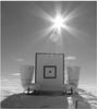 |
Fig. 1 Sodar antennas. |
Both atmospheric and optical measurements were performed during the entire winter period with some temporary interruptions. As the sodar was also used for other scientific tasks, it performed the high-resolution measurements during the second part of every month from April to October 2012 continuously over 24 h. In total, more than 2000 h of sodar observations were collected covering more than 80 days.
2.3. Seeing measurements with DIMM
To measure the seeing the DIMM is used. Two seeing monitors of DIMM type, as described by Aristidi et al. (2005b), were used in this experiment. They were located at heights of 8 m and 20 m above the surface (snow). The DIMM at 20 m has been set up on the top of the calm building of the station. They give a seeing value every 2 min. The measurements were carried out when the Sun was below the horizon.
2.4. Other measurements
To completely characterise the weather conditions, different measurements were performed. Air temperature, humidity, pressure, wind speed, and wind direction measurements are provided by the automatic weather station (AWS) Milos 520 produced by Vaisala with an acquisition rate of 1 min at heights of 1.4 m and 3.6 m above the surface for temperature and wind, respectively.
A net radiometer CNR1 produced by Kipp & Zonen was used for radiation measurements. The radiometer measures the energy balance between incoming short-wave and long-wave IR radiation versus surface-reflected short-wave and outgoing long-wave IR radiation. The CNR1 consists of a CM3 pyranometer and CG3 pyrgeometer pair that faces upward and a complementary pair that faces downward, which measure short-wave (spectral range 305−2800 nm) and far-infrared radiation (spectral range 5−50 μm), respectively. A mast equipped with the net radiometer at a height of 1.2 m and an acoustic thermoanemometer at a height of 3.5 m was installed about 15 m from the sodar antennas.
Radiosounding releases were performed every day at 1930 Local Standard Time (LST). A radiosonde RS92-GSL produced by Vaisala was used for temperature, humidity and wind measurements.
The observations performed from April to September 2012 have undergone the analysis. All data were quality controlled. A median absolute deviation filter (Barnett & Lewis 1994) was applied to remove outliers.
2.5. Characteristics of meteorological conditions
To give an indication of the statistical distributions of the relevant meteorological variables, their histograms are presented in Fig. 2.
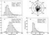 |
Fig. 2 Statistical distribution of meteorological variables. a) Temperature; b) occurrence of wind speed and direction in polar coordinates; c) pressure; d) relative humidity for the period Apr.−Sep. 2012. The intensity of the grey-scale colour in panel b) is proportional to the occurrence of the given wind speed and direction. Wind speed and direction were measured at 3.6 m; temperature, pressure and humidity at 1.4 m. |
The temperatures varied in a wide range between −80 and −30°C. The lowest temperatures of about −80°C were usually accompanied by clear-sky conditions. In spite of the absence of the sun during winter period, remarkable synoptic variations due to the intrusion of warm and moist air masses from the coastal zones occurred, accompanied by cloudiness. Elevated turbulence layers at heights of several hundred metres were observed during transition periods of synoptic perturbations.
The wind regime observed at 3.6 m was characterised mainly by low (<4 m s-1) and moderate (4 − 6 m s-1) wind speeds and directions from south and south-west sectors. Low wind speeds were observed 40% of the time and did not produce any considerable turbulence. Moderate wind speeds were observed 50% of the time and favoured intense turbulence in the lowest 10−50 m layer. The winds >6 m s-1 normally occurred during synoptic perturbations due to intrusions of maritime air masses from coastal zones with cloudiness and strong turbulence extending up to a few hundred metres.
Cloudiness is an important aspect of the weather conditions that influences the quality of astronomical observations. During the polar night the visual observations of cloudiness are difficult. To detect the presence of clouds, measurements of the downward long-wave radiation LW ↓ were performed. The values of LW ↓ were used as an objective criterion of the presence of clouds or mist. Cloudiness was occasionally registered visually by the meteorologist, in some periods photographs were made in support of the quantitative measurements of LW ↓. Figure 3 shows the histogram of the LW ↓ values measured from April to September 2012. The lowest values (<80 W m-2), when the skies were almost clear, are observed during 60% of the time; higher LW ↓ values, indicating the presence of clouds, are observed 40% of the time. The threshold of LW ↓ equal to 80 W m-2 was chosen as a point where the cumulative distribution function has a jog and the probability density function suffers a jump. There were more clouds than reported from the visual estimation of cloudiness performed in 2006 by Mosser & Aristidi (2007).
3. Results
3.1. Analysis of sodar measurements
The surface layer in the interior of Antarctica during winter is extremely stably stratified with a temperature difference between the surface and the top of the inversion reaching 20−35°C. In spite of this strong static stability, a considerable thermal optically active turbulence sometimes occurs and extends to several tens of metres. In our study we limited the consideration of the behaviour of the turbulence to the layer between 2 and 100 m.
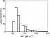 |
Fig. 3 Downward long-wave radiation for the period April−September 2012. |
3.1.1. Spatial and temporal structure of the turbulence
A general notion about the spatial and temporal distribution of the thermal optically active turbulence can be obtained just from the facsimile records of the strength of the sodar echo-signal − so called sodar echograms. These echograms (Fig. 4) show a time-height cross-section of the intensity of the backscattered signal, the intensity of grey-scale colour is proportional to the magnitude of the backscattered signal. It depicts the location pattern of temperature non-homogeneities and their evolution. For different stratification conditions of the atmosphere, various specific patterns of the thermal turbulence spatial and temporal distribution occur (e.g., Brown & Hall 1978).
First, it is possible to determine the depth of the surface-based turbulent layer (STL) from these patterns within which the highest  values occur. It can be determined visually as a height position of the black-band boundary on the echogram. There are also some computational methods to calculate this height from the numerical profiles of the echo-signal intensity. In Fig. 4, examples of typical patterns of the spatial and temporal distribution of the turbulence observed during the winter period are shown. The vertical profiles of that correspond to the considered spatial and temporal patterns of the turbulence are shown in Fig. 5.
The first case (Fig. 4a) is a very weak turbulence, when the STL does not extend higher than 2−3 m (between 1500 and 1800 LST). The meteorological conditions that favour to this situation are characterised by weak wind <2 m s-1 , and the temperature values in these situations are low (around −70°C). In this period the seeing was about 0.38 arcsec. Typically, under such conditions the seeing values range within 0.3−0.6 arcsec.
The other case (Fig. 4b) is a shallow, but distinguishable STL extending not higher than 10−15 m. The seeing values observed at 8 m are >1 arcsec, but at 20 m they remain <1 arcsec. The third case is a well-distinguishable STL extending up to 20−70 m (Fig. 4c). The moderate wind 3−6 m s-1 characterises meteorological conditions for this situation. Seeing values higher than 1 arcsec at 8 and 20 m were observed under these conditions. The fourth, less typical, situation is shown in Fig. 4d, when elevated turbulent layers (ETL) are observed above the STL and can occur at heights between 30−100 m.
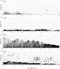 |
Fig. 4 Some typical cross-section patterns of the surface-based turbulent layer depicted by sodar echograms. The grey-scale intensity is proportional to the strength of the thermal optically active turbulence characterised by the structure refraction index parameter |

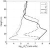 |
Fig. 5 Typical vertical profiles of |
Histograms showing the statistical distribution of the STL depth are given in Fig. 6a. STL deeper than 20 m were observed at 45% of the total time, STL with a depth lower than 20 m − 55%, and less than 5 m − 17%. We have to note that the STL occupies only the lowest part of the temperature inversion layer. Figure 6b shows the histogram of heights of the surface-based temperature inversion determined from daily measured radiosonde profiles. The main statistical parameters of the considered quantities are given in Table 1. The mean STL depth and inversion height are 23 m and 133 m, respectively; the median values are 16 m and 125 m, respectively. On average, the STL depth is about 6−7 times lower than the inversion layer height.
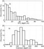 |
Fig. 6 a) Depth of the surface turbulent layer (from the sodar) and b) height of the temperature inversion layer (from 183 daily radiosonde measurements) for April−September 2012. |
Now we consider how the STL depth depends on the relevant atmospheric variables temperature and wind speed. In Fig. 7a, the STL depth values are plotted versus the temperature values for the period from May to September. The lowest STL depth values <5 m are observed mainly at temperatures <−65°C. There is no general correlation between the STL depth and temperature. The wind speed appears to be a more relevant variable that influences the STL depth. Figure 7b shows the STL depth versus wind speed values. The STL depth increases when the wind intensifies. When the wind speed reaches >4 m s-1 , the STL extends higher than 20 m. The correlation coefficient is estimated to be 0.72 with the bounds for a 95% confidence interval of 0.65 and 0.79.
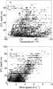 |
Fig. 7 Depth of the surface-based turbulent layer versus a) temperature at 1.4 m and b) wind speed at 3.5 m for the period April−September 2012. |
Averages of the depths of the surface-based turbulent layer and the temperature-inversion layer estimated for the period April−September 2012.
3.1.2. Processing the sodar C profiles
To obtain the behaviour of vertical profiles of and the TOF values, the profiles of the received signal intensity were processed using a multi-step procedure. The signal received by sodar is a mix of the echo-signal and the ambient acoustic noise. As an estimate of the noise level, we used the intensity of the received signal averaged over the highest range gates where the echo-signal intensity usually was negligible. The noise intensity level was then subtracted from the received signal intensity at all the range gates. The second step is the correction to compensate for the attenuation of the transmitted signal due to non-complete intersection of the beams of separated transmitting antennae at the lowest heights. The third step is the calculation of range-corrected intensity profiles, which are obtained by multiplying the intensity values by the h2 factor. This is due to the spherical convergence with a distance of the transmitted acoustic wave (e.g., Brown & Hall 1978). At the next step the signal intensity is corrected for the attenuation of the acoustic signal caused by sound absorption in the air. After these corrections the obtained values are proportional to along the whole profile. The profiles shown in Fig. 5 have been produced this way.
Profiles of  are obtained from using the relationship given in Sect. 1. The TOF values were calculated for different height intervals to determine the relative contribution of different atmospheric layers to the seeing. The histograms of TOF values (in arbitrary units) for three height intervals of 2−15 m, 2−30 m and 2−70 m are shown in Fig. 8. The integral turbulence intensities inside the layers of 2−30 m and 2−70 m do not differ significantly, but are somewhat higher than the intensity in the 2−15 m layer. This means that turbulence between 15 and 30 m contributes appreciably to the image distortion in addition to the more intense turbulence at lower heights <15 m.
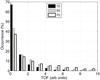 |
Fig. 8 Sodar TOF values within the layers: 1) 2−15 m; 2) 2−30 m; and 3) 2−70 m for the period April−September 2012. |
Figure 9 shows TOF values for the 2−100 m layer versus the wind speed at 3.5 m for the period from April to September 2012. On average, the TOF values increase with increasing values of the wind speed. But the dependence of TOF on wind speed is not monotonous. It is possible to distinguish two specific ranges of values of the wind speed with a different behaviour of the TOF values. One range can be specified to be between 0 and 4 m s-1, the other >4 m s-1. Within the first cluster TOF values are distributed almost uniformly in a wide range between the lowest and highest values showing a slow increase with wind intensity. The second cluster is characterised by significantly higher TOFs, which are mainly concentrated in a narrow range. The wind speed seems to be the most relevant meteorological parameter favouring the generation of intense optically active turbulence in the lowest several tens of metres under very stable stratification.
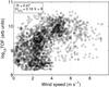 |
Fig. 9 TOF values in the layer 2−100 m (from the sodar) versus wind speed at 3.5 m for the period April−September 2012. |
Averages of the seeing estimated during April−September 2012.
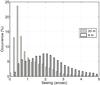 |
Fig. 10 2-min seeing values measured at 8 m and 20 m for the period April−September 2012. |
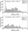 |
Fig. 11 Seeing values for a) a clear sky and b) a slightly cloudy sky. |
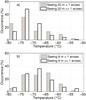 |
Fig. 12 Temperature for good and bad seeing values at a) 20 m and b) 8 m. |
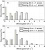 |
Fig. 13 Wind speed for good and bad seeing values at a) 20 m and b) 8 m. |
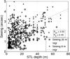 |
Fig. 14 Seeing values at 8 m and 20 m as a function of the sodar STL depth. Dashed lines show the corresponding regressions. |
3.2. Analysis of optical measurements and their dependence on weather conditions
The histograms in Fig. 10 show the statistical distribution of the seeing values measured at heights of 8 m and 20 m for the period from April to September 2012. The total number of data was 17 486 and 10 799 at 8 m and 20 m, respectively. The arithmetic mean, median, geometric mean, and standard deviation values for both heights are reported in Table 2. The results show a considerable difference in the quality of astronomical observations at the two heights. The seeing values at 8 m are distributed almost uniformly over a range between 0.5 and 3 arcsec where >80% of the data are concentrated. In contrast, the seeing values at 20 m show a remarkable narrow peak around 0.5 arcsec. More than 50% of data are concentrated between 0.2 and 1 arcsec, and about 40% are located between 0.4 and 0.8 arcsec. The median value at 20 m is 0.8 arcsec and about twice lower than that at 8 m. There is a peak around a seeing of 0.5 arcsec exists for the 8 m measurements, but it is significantly lower than at 20 m.
The histograms in Fig. 11 show the statistical distributions of seeing values at two heights separately for clear-sky and slightly cloudy conditions. The statistical distributions at both heights are rather similar for both sky conditions. We conclude that light cloudiness does not influence the seeing.
The histograms in Fig. 12 show the temperature distribution in different seeing conditions (“good” , i.e. <1 arcsec, and “bad”, i.e. ≥ 1 arcsec) at both heights. For the 8m-DIMM, the temperature distribution is similar for good and bad seeings. At 20 m the good seeing values occur mainly for the lowest temperatures, which range between −80 and −70°C, the bad seeing was observed mainly between −75 and −65°C.
The histograms in Fig. 13 show the distribution of the wind speed with the same seeing filter. At 20 m good values occur mainly for the lowest wind speeds <3 m s-1, the most bad seeing conditions were observed for wind speeds >2 m s-1. At 8 m, it is interesting to note that good seeing conditions are not observed when the wind speed is >4 m s-1.
 |
Fig. 15 Evolution of the STL structure shown by sodar echograms on August 20, 2012. |
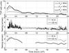 |
Fig. 16 Time series of a) the turbulent optical factor measured by the sodar for three layers (averaged over time intervals of 1 h), and the seeing measured by DIMMs: b) 2-min averages, c) 1-h averages, on August 20, 2012. |
3.3. Correlation between seeing from DIMM and turbulence strength measured by sodar
In this paragraph we consider the principal topic of this study: how the characteristics of the optically active turbulence determined with a sodar correlate with the seeing measured directly by the DIMM.
First, we analyse the correlation between the depth of the STL estimated from sodar echograms and seeing. The graph in Fig. 14 shows seeing values measured at two heights against the STL depth measured by the sodar. These data show that the best image quality (the lowest seeing values) are observed for lower STL depths. The median seeing obtained in cases when the 20−m DIMM was above the STL is estimated from our measurements to be ≈0.63 arcsec.
The correlation coefficients of ≈0.5 are reliable but not very high. From this we can conclude that the STL depth itself is not sufficient to explain the seeing values. Visual inspection of the sodar echograms has indeed shown that the turbulence intensity within STL of the same depths can differ significantly. The more important characteristics probably is the total turbulence strength integrated over the STL, which is characterised by the TOF values.
First, we consider one case showing an obvious correlation between seeing values and the turbulence determined with the sodar. As an example, we present the results obtained on 20 August 2012 when the structure of the STL and the seeing changed considerably during 24 h. The evolution of the spatial and temporal structure of the STL is shown on sodar echograms in Fig. 15.
Synchronous time series of the sodar TOF and seeing from DIMM measurements are shown in Fig. 16. The TOF for three layers are given: 1) [2 m, 30 m], 2) [2 m, 40 m], and 3) [2 m, 50 m]. The TOF values are averaged over 1 h. The night period is characterised by an STL of 40−50 m depth with intense turbulence within it. Corresponding seeing values are considerably higher than 1 arcsec. Later, the STL depth and the turbulence intensity decrease. During the day and evening hours TOF continue to decrease. The seeing values show a similar time behaviour.
In Fig. 17, seeing values versus TOF calculated for the layer [2 m, 50 m] are shown. The correlation coefficients are 0.93 and 0.79 for seeing at 20 m and 8 m, respectively. The bounds of the correlation coefficients for a 95% confidence interval are estimated to be 0.85 and 0.95 for 20 m, and 0.65 and 0.84 for 8 m. This shows the reliable correlation between seeing and TOF values.
Summarised seeing values versus TOF values for the entire observational period are shown in Fig. 18. The presented TOF was calculated for the 2−40 m layer. The lowest seeing of <1 arcsec is observed when the TOF has the lowest values. Higher seeing values occur when the TOF increases. The correlation coefficients are estimated to be 0.76 and 0.56 for seeing at 20 m and 8 m, respectively. The bounds of the correlation coefficients for a 95% confidence interval are estimated to be 0.67 and 0.82 for 20 m and 0.50 and 0.62 for 8 m. Testing the hypothesis of no correlation shows that this correlation is significant for both data sets. Here again, a clear connection is found between seeing and the sodar TOF values.
The TOF is a more relevant parameter than the STL depth to describe the influence of the optically active turbulence on the image quality.
4. Summary and conclusions
The influence of the optically active atmospheric turbulence due to temperature fluctuations in the atmospheric boundary layer on the quality of astronomical observations at the Concordia station was studied using the measurements made during the field experiment carried out over the entire winter period of 2012. For the first time, optical measurements of the seeing made by two seeing monitors (DIMM) at two levels, 8 m and 20 m, were accompanied by remote observations of the spatial and temporal pattern of the thermal turbulence by a high-resolution sodar within the lowest hundred metres beginning from 2 m above the surface.
Although the boundary layer in the interior of Antarctica during the winter is very stably stratified with an inversion strength of 20−35°C, considerable optically active turbulence sometimes occurs and extends from the surface up to several tens of metres. Typical patterns of the spatial and temporal distribution of turbulence shown by sodar echograms were analysed and classified according to their intensity and vertical extension. Statistics of the depth of the STL were determined. It was shown that both the STL depth and the TOF within it (for the first 100 m) increase with increasing values of the wind speed. Surface-based turbulent layers with a depth 1) lower than 5 m are observed for ≈17% of time; 2) between 5 m and 20 m for 38%; 3) and higher than 20 m for 45%. Elevated turbulent layers at heights of 50−100 m occur for 5% of the total time.
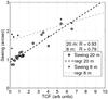 |
Fig. 17 Correlation between the seeing values measured with DIMM at the two heights and the sodar TOF estimated within the layer between 2 m and 50 m for August 20, 2012. |
The analysis of the seeing from the two DIMM evidences the essential difference in the quality of astronomical observations at the two heights. The median seeing value at 8 m is ≈2.1 arcsec, at 20 m it is significantly lower (0.8 arcsec).
A reliable correlation exists between the seeing and the intensity of the thermal turbulence measured by the sodar. The best seeing values are accompanied by the lowest depth of the STL and lowest values of TOF. From these results it is possible to conclude that turbulence within the lowest layer of a few tens of metres is responsible for the main part of the bad seeing at Dome C. This is consistent with the previous studies by Trinquet et al. (2008) and Aristidi et al. (2009).
The relative contribution of different height layers to the image distortion was considered. Based on the statistics of the turbulent optical factor for different height intervals within the
surface layer, we can estimate that a telescope located at an altitude of 20 m will be above the STL for 55% of the time. The median seeing obtained in this case is estimated from our measurements to be ≈0.63 arcsec.
Acknowledgments
This research was supported by the Italian National Research Programme (PNRA) and the French Polar Institute (IPEV) as part of French-Italian projects for Dome C. The authors thank A. Conidi, N. Ferrara, and S. Ciampichetti for the technical support provided in the realization of the sodar antennas and the logistics staff of the Concordia station during the field work. We also wish to cite the people who participated in the setup of the instruments during the summer campaign: F. X. Schmider, D. Mekarnia, and G. Cohen from our industrial partner “Optique et Vision”. A special thanks to M. A. Kallistratova for her contribution to the development of the sodar method, and for useful discussions and remarks.
References
- Agabi, A., Aristidi, E., Azouit, M., et al. 2006, PASP, 118, 344 [NASA ADS] [CrossRef] [Google Scholar]
- Argentini, S., & Pietroni, I. 2010, EAS Pub. Ser., 50, 45 [CrossRef] [EDP Sciences] [Google Scholar]
- Argentini, S., Petenko, I. V., Mastrantonio, G., Bezverkhnii, V. A., & Viola, A. P. 2001, J. Geophys. Res. Atmos., 106, 12463 [NASA ADS] [CrossRef] [Google Scholar]
- Argentini, S., Mastrantonio, G., Petenko, I., Pietroni, I., & Viola, A. 2012, Boundary-Layer Meteorol., 143, 177 [NASA ADS] [CrossRef] [Google Scholar]
- Aristidi, E., Agabi, A., Vernin, J., et al. 2003, A&A, 406, L19 [NASA ADS] [CrossRef] [EDP Sciences] [Google Scholar]
- Aristidi, E., Agabi, A., Fossat, E., et al. 2005a, A&A, 444, 651 [NASA ADS] [CrossRef] [EDP Sciences] [Google Scholar]
- Aristidi, E., Agabi, K., Azouit, M., et al. 2005b, A&A, 430, 739 [NASA ADS] [CrossRef] [EDP Sciences] [Google Scholar]
- Aristidi, E., Fossat, E., Agabi, A., et al. 2009, A&A, 499, 955 [NASA ADS] [CrossRef] [EDP Sciences] [Google Scholar]
- Barnett, V., & Lewis, T. 1994, Outliers in statistical data (New York: Wiley), 3 [Google Scholar]
- Brown, E. H., & Hall, F. F. 1978, Rev. Geophys., 16, 47 [NASA ADS] [CrossRef] [Google Scholar]
- Genthon, C., Six, D., Gallée, H., Grigioni, P., & Pellegrini, A. 2013, J. Geophys. Res. Atmos., 118, 685 [CrossRef] [Google Scholar]
- Gur’yanov, A. E., Irkaev, B. N., Kallistratova, M. A., et al. 1988, Sov. Astron., 32, 328 [NASA ADS] [Google Scholar]
- Gur’yanov, A., Kallistratova, M., Kutyrev, A., et al. 1992, A&A, 262, 373 [NASA ADS] [Google Scholar]
- Lawrence, J. S., Ashley, M. C., Tokovinin, A., & Travouillon, T. 2004, Nature, 431, 278 [NASA ADS] [CrossRef] [PubMed] [Google Scholar]
- Martin, H. 1987, PASP, 99, 1360 [NASA ADS] [CrossRef] [Google Scholar]
- Mosser, B., & Aristidi, E. 2007, PASP, 119, 127 [NASA ADS] [CrossRef] [Google Scholar]
- Tatarskii, V. I. 1971, The Effects of the Turbulent Atmosphere on Wave Propagation (Jerusalem: Israel Program for Scientific Translation), 472 [Google Scholar]
- Trinquet, H., Agabi, A., Vernin, J., et al. 2008, PASP, 120, 203 [NASA ADS] [CrossRef] [Google Scholar]
All Tables
Averages of the depths of the surface-based turbulent layer and the temperature-inversion layer estimated for the period April−September 2012.
All Figures
|
Fig. 1 Sodar antennas. |
| In the text | |
|
Fig. 2 Statistical distribution of meteorological variables. a) Temperature; b) occurrence of wind speed and direction in polar coordinates; c) pressure; d) relative humidity for the period Apr.−Sep. 2012. The intensity of the grey-scale colour in panel b) is proportional to the occurrence of the given wind speed and direction. Wind speed and direction were measured at 3.6 m; temperature, pressure and humidity at 1.4 m. |
| In the text | |
|
Fig. 3 Downward long-wave radiation for the period April−September 2012. |
| In the text | |
|
Fig. 4 Some typical cross-section patterns of the surface-based turbulent layer depicted by sodar echograms. The grey-scale intensity is proportional to the strength of the thermal optically active turbulence characterised by the structure refraction index parameter |
| In the text | |
|
Fig. 5 Typical vertical profiles of |
| In the text | |
|
Fig. 6 a) Depth of the surface turbulent layer (from the sodar) and b) height of the temperature inversion layer (from 183 daily radiosonde measurements) for April−September 2012. |
| In the text | |
|
Fig. 7 Depth of the surface-based turbulent layer versus a) temperature at 1.4 m and b) wind speed at 3.5 m for the period April−September 2012. |
| In the text | |
|
Fig. 8 Sodar TOF values within the layers: 1) 2−15 m; 2) 2−30 m; and 3) 2−70 m for the period April−September 2012. |
| In the text | |
|
Fig. 9 TOF values in the layer 2−100 m (from the sodar) versus wind speed at 3.5 m for the period April−September 2012. |
| In the text | |
|
Fig. 10 2-min seeing values measured at 8 m and 20 m for the period April−September 2012. |
| In the text | |
|
Fig. 11 Seeing values for a) a clear sky and b) a slightly cloudy sky. |
| In the text | |
|
Fig. 12 Temperature for good and bad seeing values at a) 20 m and b) 8 m. |
| In the text | |
|
Fig. 13 Wind speed for good and bad seeing values at a) 20 m and b) 8 m. |
| In the text | |
|
Fig. 14 Seeing values at 8 m and 20 m as a function of the sodar STL depth. Dashed lines show the corresponding regressions. |
| In the text | |
|
Fig. 15 Evolution of the STL structure shown by sodar echograms on August 20, 2012. |
| In the text | |
|
Fig. 16 Time series of a) the turbulent optical factor measured by the sodar for three layers (averaged over time intervals of 1 h), and the seeing measured by DIMMs: b) 2-min averages, c) 1-h averages, on August 20, 2012. |
| In the text | |
|
Fig. 17 Correlation between the seeing values measured with DIMM at the two heights and the sodar TOF estimated within the layer between 2 m and 50 m for August 20, 2012. |
| In the text | |
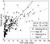 |
Fig. 18 Same as Fig. 17, but for the whole period from April to September 2012. |
| In the text | |
Current usage metrics show cumulative count of Article Views (full-text article views including HTML views, PDF and ePub downloads, according to the available data) and Abstracts Views on Vision4Press platform.
Data correspond to usage on the plateform after 2015. The current usage metrics is available 48-96 hours after online publication and is updated daily on week days.
Initial download of the metrics may take a while.