| Issue |
A&A
Volume 567, July 2014
|
|
|---|---|---|
| Article Number | A9 | |
| Number of page(s) | 8 | |
| Section | The Sun | |
| DOI | https://doi.org/10.1051/0004-6361/201423449 | |
| Published online | 04 July 2014 | |
Stereoscopic observations of the effects of a halo CME on the solar coronal structure⋆
INAF – Catania Astrophysical Observatory, 95123 Catania, Italy
e-mail: sdo@oact.inaf.if
Received: 17 January 2014
Accepted: 29 April 2014
We investigated the substantial restructuring of the outer solar corona in the aftermath of the halo CME that occurred on 9 March 2012. To perform our analysis, we used SOHO/LASCO, STEREO/COR1 and SDO/AIA data, which provide observations from different viewpoints. In particular, we applied the polarization ratio technique to the COR1 calibrated images to derive the three-dimensional structure of the CME and determine its direction and speed of propagation. We also estimated the CME mass from a sequence of four observations of the event and obtained values of up to 2.2 × 10¹⁶ g. The COR1 images show a brightness decrease in the coronal sector where the CME propagates. We verified that this intensity reduction is due to a plasma depletion. Moreover, the combined analysis performed by the two STEREO satellites allowed us to deduce that a preexisting streamer is located along the propagation direction of the CME and disappears after the passage of the event. The coronal mass loss associated with the plasma depletion is much lower than the mass expelled from the Sun in the COR1-B data. Conversely, the COR1-A obsevations allowed us to infer that the mass of the streamer carried away from the outer corona corresponds to about half of the CME mass. The results highlight the importance of stereoscopic observations in the study of corona restructuring in the aftermath of a CME event.
Key words: Sun: activity / Sun: corona / Sun: coronal mass ejections (CMEs)
The movie associated with Fig. 3 is available in electronic form at http://www.aanda.org
© ESO, 2014
1. Introduction
Coronal mass ejections (CMEs) consist of large plasma structures that are expelled from the Sun. There are two main purposes for studying CMEs: the first is to investigate the prominent role that they play in solar activity, the second is to achieve reliable space weather predictions on Earth. In fact, CMEs remove stored magnetic energy and plasma from the solar corona and carry them into the heliosphere (Low 1996), causing major transient disturbances. An open question is understanding whether CMEs respond passively or contribute dynamically to the coronal field restructuring (Liu et al. 2009). Low (1996, 1997, 2001) considered CMEs to be a basic mechanism of coronal magnetic field evolution, whereas Sime (1989) suggested that the global coronal field organization does not respond in a lasting way to CMEs, because the mass and energy of a CME are much smaller than those of the corona. Subramanian et al. (1999) examined coronagraphic images of CMEs from January 1996 to June 1998 to study the relationship between CMEs and coronal streamers; the authors observed both CMEs that disrupt streamers and CMEs that have no apparent effect on them.
In general, the observations indicate that the possible effects of CMEs on the coronal structure evolution can be the so-called coronal dimming, observable on the solar disk in X-ray, EUV, and Hα emission, and theplasma depletion in the outer corona. These phenomena are shortlived, and their lifetimes vary from shorter than one day to longer than three days (Sterling & Hudson 1997). Some measurements imply that the dimming, as well as the depletion, is caused by an effective mass loss from the low corona (Hudson & Webb 1997) instead of by a plasma temperature decrease (e.g. Harrison & Lyons 2000; Harrison et al. 2003). It is likely that the portion of mass that leaves the low corona becomes part of the CME (e.g. Webb et al. 2000), but the details of the process are still uncertain. Coronal dimmings and depletions have not been observed as frequently as their associated eruptive phenomena, but very recent results (e.g. Schrijver & Title 2011) suggest that they are more common occurrences than what is expected from previous measurements. The detection of the regions involved in the coronal dimming also allows accurate mapping of the areas where CMEs are triggered on the solar disk (Thompson et al. 2000; Harrison et al. 2003). Ramesh & Sastry (2000) carried out the first low-frequency radio observations of a plasma depletion that occurred in the outer solar corona and verified a complete restructuring of the corona in less than 24 h. They estimated the mass loss associated with the depletion and found that it agrees well with the value obtained through white-light observations of the event.
The main goal of this paper is to study the effects of a CME on the structure of the solar corona, observing its configuration before, during, and after the halo CME that occurred on 9 March 2012. We use observations of this event in the low and outer corona, performed by several instruments from different viewpoints. We especially exploit the new-generation data from the Solar TErrestrial RElations Observatory (STEREO; Kaiser et al. 2008) to derive the three-dimensional structure of the CME and determine its direction and speed of propagation. The STEREO coronagraphic images show a brightness decrease in the coronal sector involved in the passage of the CME. In addition, the observations indicate that the eruption disrupts a preexisting streamer, visible in the portion of the COR1-A field of view (FOV), and that is subsequently affected by the CME propagation. We investigate the characteristics of this brightness reduction, also making use of the other measured properties of the CME, such as location relative to the solar disk, angular width, speed, and column density.
2. Observations
On 9 March 2012 a halo CME was observed from 4:26 UT to 6:26 UT by the Large Angle and Spectrometric Coronagraph (LASCO; Brueckner et al. 1995) on board the SOlar and Heliospheric Observatory (SOHO). Figure 1 shows the image of the CME taken by the C2 coronagraph of LASCO at 4:50 UT; the annular FOV of the instrument ranges from 2.5 to 6.5 R⊙. This event seems to be associated (in time) with an M6.3 class flare detected by the Geostationary Operational Environmental Satellite (GOES). The plot in Fig. 2 depicts the X-ray (1–8 Å) emission registered by GOES: the rapid increase corresponds to the flare onset (~3:25 UT), while the red and black vertical lines indicate the time of the peak of the flare (3:53 UT) and the beginning of the LASCO/C2 observations of the CME (4:26 UT). The event was also observed on the solar disk by the Atmospheric Imaging Assembly (AIA; Lemen et al. 2012) on board the Solar Dynamics Observatory (SDO). SDO/AIA on-disk observations show the evolution of the active region NOAA 11429 in the aftermath of the M6.3 class flare. This active region is indicated by the arrow in Fig. 3, which shows the AIA 193 Å image at 3:42 UT, that is, at the starting time of a coronal wave on the solar disk (see the online movie), which corresponds to the beginning of the plasma ejection.
 |
Fig. 1 LASCO/C2 image at 4:50 UT on 9 March 2012. The white circle outlines the limb of the solar disk. |
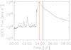 |
Fig. 2 GOES X-ray (1–8 Å) emission from 0:00 UT to 8:00 UT on 9 March 2012. The flare onset (~3:25 UT) corresponds to the rapid flux increase. The red vertical line indicates the time of the peak of the flare (3:53 UT), while the black vertical line coincides with the beginning of the LASCO/C2 observation of the CME (4:26 UT). |
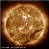 |
Fig. 3 SDO/AIA 193 Å image at 3:42 UT on 9 March 2012. The arrow points out active region NOAA 11429. An animation showing the coronal wave by running difference images is available online. |
The region of the CME event was also investigated, from 3:30 UT to 24:00 UT with 5-min time cadence, using data from the COR1 coronagraphs on board the two STEREO spacecraft. There is a gap in the COR1-A data from 4:05 UT to 18:00 UT. Figure 4 shows the positions of STEREO Ahead (red) and Behind (blue) satellites at the epoch of the observations considered in this paper and relative to the Sun (yellow) and Earth (green): the spacecraft were approximately positioned on the ecliptic plane and separated by an angular distance of about 230°, measured clockwise from A to B. The COR1 coronagraphs, whose annular fields of view range from 1.4 to 4.0 R⊙, take simultaneous sequences of three polarized images, which can be combined to give total brightness or polarized brightness images. Figure 5 shows the images of the corona as seen by both STEREO/COR1, at 3:40 UT (before the CME, top panels) and at 4:00 UT (during the CME, bottom panels).
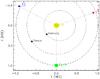 |
Fig. 4 Positions of the STEREO Ahead (red) and Behind (blue) spacecrafts relative to the Sun (yellow) and Earth (green) on 9 March 2012. Distances are in astronomical units in a Cartesian heliocentric Earth ecliptic (HEE) coordinate system. |
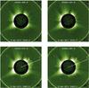 |
Fig. 5 STEREO/COR1 Ahead (left) and Behind (right) images at 3:40 UT (before the CME, top panels) and at 4:00 UT (during the CME, bottom panels). The arrow in the image of the top-left panel points at a faint and short streamer visible in the FOV of COR1-A, before the CME propagation. In the images of the bottom panels, paths 1 are along a radial direction at 73° and 290° PA (measured counterclockwise from North) in the FOV of COR1-A and COR1-B, while paths 2 are perpendicular to the respective paths 1 and extend from 42° to 104° PA and from 257° to 323° PA in the FOV of COR1-A and COR1-B. |
3. Data analysis and results
The position of active region NOAA 11429 (see Fig. 3) indicates that the CME started near the central meridian of the Sun (0° in heliographic longitude). The stereoscopic view provided by the STEREO satellites should allow determining the direction of propagation of the CME and compute its true speed, and not the speed projected onto the plane of the sky (POS) of a single coronagraph. Nevertheless, the position of the STEREO spacecraft does not allow computing any local correlations of the event from stereoscopic analysis. The Ahead and Behind spacecrafts were located very close to the ecliptic plane and separated from the Sun-Earth line (also lying on the ecliptic plane and where LASCO is placed) by an angular distance of about 110° (measured counterclockwise) and 120° (measured clockwise).
In spite of this, however, we are able to investigate the three-dimensional structure of the CME and study its kinematics by applying the polarization ratio technique (e.g. Moran & Davila 2004; Mierla et al. 2009) to the COR1 data. This method gives no information about the depth extent of the CME along the line of sight (LOS), but allows us to obtain a weighted mean angular distance of the ejected plasma from the POS of the two STEREO spacecrafts. This distance is used to derive the plasma density and, consequently, the mass of the CME from the COR1 brightness images.
3.1. 3D reconstruction by the polarization ratio technique
To investigate the spatial configuration of the considered CME, we measured the ratio of polarized to unpolarized brightness obtained from the STEREO/COR1 observations. As in Billings (1966), denoting by Bt and Br the tangential and radial components of the scattered radiance, the polarized brightness is given by pB = Bt − Br and the unpolarized brightness by uB = B − pB = (Bt + Br) − (Bt − Br) = 2 Br. We applied the polarization ratio technique (Moran & Davila 2004; Mierla et al. 2009) to derive the 3D structure of the CME. This technique takes into account that the degree of polarization of the Thomson-scattered light by coronal electrons (K-corona) is a function of the scattering angle between the incident light direction and the direction towards the observer (Billings 1966), which in turn is a function of the effective distance of the scattering coronal electrons from the plane of the sky, once a LOS is selected.
We computed the polarization ratio on four COR1-A and -B calibrated images taken from 3:50 UT to 4:05 UT with 5-min time cadence. The COR1 calibration (Thompson & Reginald 2008) includes a monthly minimum-intensity subtraction from the data; with this we ensured that the brightness is not affected by scattering from dust particles (F-corona) or by stray-light. We applied the polarization ratio technique separately to the COR1-A and -B images. As suggested by Mierla et al. (2009), to remove preexisting steady structures, such as streamers, we subtracted a minimum-intensity image from the total and polarized brightness images by taking the lowest brightness value among the images taken before and during the event pixel by pixel. In addition, a 5 × 5 median filter was applied to enhance the signal-to-noise ratio of these difference images. We used the routine eltheory.pro, available in the SolarSoftware library, which exploits the Thomson-scattering theory to compute the value of the total or polarized brightness for a single electron, as a function of the distance of this electron from the Sun center (e.g. Minnaert 1930; Van De Hulst 1950). For each image, the polarized-to-unpolarized brightness ratio obtained from the observations was computed pixel by pixel (which means along the respective lines of sight) and compared with the theoretical values obtained from the Thomson-scattering theory. These values are a function of the distance of the coronal electron from the plane of the sky: the distance for which the difference between observed and theoretical brightness ratio is smallest corresponds to the most probable location of the coronal electron. Owing to the forward/backward symmetry of the Thomson scattering, any scattering angle θ (angular distance ahead of the POS) allows a second solution −θ (angular distance behind the POS) for this technique. But this ambiguity can be solved when the propagation direction of the CME with respect to the POS is known. This can be accomplished, for instance, using on-disk observations, which provide information about the region of triggering, and/or coronagraphic observations from different spacecraft, which give one more point of view on how the event moves throughout the solar corona.
We obtained one 3D reconstruction of the CME from each COR1 calibrated image. The results of our computation show that the bulk of the emission by the portion of the ejected plasma as seen by each spacecraft comes from a mean angular distance equal to θA = +16° from the POS of STEREO-A and θB = +24° from the POS of STEREO-B. Owing to the forward/backward symmetry of the Thomson scattering, the emission might come, similarly, from  and
and  . The AIA and LASCO/C2 observations help us to solve this geometric ambiguity: we know how the event propagates in the LASCO/C2 plane of the sky and that the time interval between the beginning of the event as observed by AIA (3:42 UT) and its appearance in the LASCO/C2 FOV (4:26 UT) is about 45 min. The temporal sequence of the 3D reconstructions obtained by the polarization ratio technique allows us to outline the location of the CME front and calculate its speed of propagation; we find that the plasma moves in the FOV of both COR1 coronagraphs with an average speed of about 1000 km s-1. With this in mind, we can estimate that as sketched in Fig. 6, plasma propagating at 36° in heliographic longitude (which corresponds to θA = + 16°) would appear to run across a distance sC2 ≃ 2.5 R⊙ in the LASCO/C2 POS during a time interval of 45 min. Conversely, if this plasma propagates at 4° in heliographic longitude (which corresponds to ), it would appear to run across a distance
  R⊙ in the same time. Then, on the basis of AIA and LASCO/C2 observations, we can conclude that the bulk of the emission in COR1-A comes from θA = + 16°. Based on similar arguments, the mean angular distance from the POS of STEREO-B would be , which corresponds to −6° in heliographic longitude.
Summarizing, from on-disk and coronagraphic observations together with kinematics analysis, we determine that the CME emission distribution covers 42° in heliographic longitude, from −6° to 36°. Figure 7 shows the 3D reconstruction of the CME at 4:00 UT, obtained by the polarization ratio technique applied to the COR1-A and -B data. The 3D plot (see Mierla et al. 2009) is in a Cartesian heliocentric Earth equatorial (HEEQ) coordinate system, where the X-axis points towards Earth. In the plot, the Sun is represented by the gray sphere, and the reconstructed ejected plasma is sketched in a color scale that only depends on its heliocentric distance (lighter meaning closer to the Sun center). The radius of the outer gridded sphere is 1.4 R⊙, which is the radius of the COR1 occulter. As described before, we have no information about the depth extent of the CME by the polarization ratio technique, but rather a weighted mean distance of the ejected plasma along each line of sight. Therefore, the outputs of the 3D reconstruction (see Fig. 7) turn out to be just two rough elongated surfaces, which extend over about 80° in heliographic latitude and approximately represent the boundaries of the CME emission distribution in longitude (~42°).
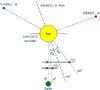 |
Fig. 6 Sun-STEREO satellites and Sun-Earth directions (short-dashed lines), the STEREO-A POS direction (long-dashed line) and the north polar view of the LASCO/C2 occulter (solid line). The solid blue lines indicate the two possible propagation directions of the ejected plasma at the mean angular distances θA and |


 |
Fig. 7 3D reconstruction of the CME, obtained by the polarization ratio technique applied to the COR1-A and -B data at 4:00 UT. The gray sphere represents the Sun. The numbers on the sphere are the values of HEEQ longitudes, where the X-axis points towards the Earth. The radius of the outer gridded sphere is 1.4 R⊙. |
3.2. CME mass and column density estimates
After the 3D structure and the direction of propagation of the CME were determined, we exploited this information to calculate its mass. We used the routine scc_calc_cme_mass.pro, available in the SolarSoftware library, which calculates the number of electrons providing the measured brightness in each pixel of the COR1 images. We used the results of the polarization ratio technique as input to the routine: since the Thomson scattering is a sensitive function of the plasma location, we set the mean angular distances of the ejected plasma from the planes of the sky of STEREO-A and -B spacecraft, that are θA = + 16° and θB = −24° (hereafter θ is denoted without apex). The scc_calc_cme_mass.pro routine recalls eltheory.pro, which computes the value of the brightness for a single electron, assuming that the location of this electron is the fixed angular distance from the POS along the respective line of sight, as described before. Pixel by pixel, the ratio between the COR1 brightness and the brightness calculated by the eltheory.pro routine gives the number of electrons providing the COR1 brightness, assuming that all these electrons are located at fixed angular distance from the POS, that is, θA and θB for COR1-A and -B. We can therefore derive the CME mass by adding the number of electrons over the CME area and multiplying by the electron mass. We selected in the COR1 calibrated images the CME area, which is the one delimited by the CME front and the subtended circular sector of the COR1 occulter. Then, we calculated four values of the mass at different times, corresponding to the four observations carried out in the time interval 3:50–4:05 UT. No artifact such as filtering and intensity removing was applied on the COR1 images. The results, reported in Table 1, indicate that the mass values increase with time, as more and more plasma is ejected and appears in the COR1 FOV. However, we cannot neglect the contributions from plasma accretion or plasma pileup ahead of the CME flux rope. In addition, note that the mass value measured by COR1-A is larger than that measured by COR1-B at the relevant time, because the event appears earlier and is more developed in the COR1-A FOV.
CME mass values in grams calculated at different times, corresponding to the four COR1 observations in the time interval 3:50–4:05 UT.
From the number of electrons that provide the measured brightness in each pixel of the considered COR1 calibrated images, it is possible to derive the number of electrons per square centimeter (electrons cm-2), i.e. the column density, for each pixel if one knows the pixel size. We used this quantity to investigate the properties of the CME propagation in the solar corona. During the time interval 3:50–4:05 UT, the CME moved in the FOVs of both COR1 coronagraphs and its front reached different positions along different paths, such as those reported in the images of the bottom panels of Fig. 5 and indicated by the numbers 1 and 2. The paths 1 were chosen along a radial direction at 73° and 290° position angle (PA, measured counterclockwise from the north pole) in the FOV of COR1-A and COR1-B, respectively; in so doing, the CME turns out to be axially symmetric with respect to them, in both FOV. The paths 2 are perpendicular to the respective paths 1 and extend from 42° to 104° PA and from 257° to 323° PA in the FOV of COR1-A and COR1-B, respectively.
Figure 8 shows the column density as a function of the distance projected on the plane of the sky along the paths 1 at different times. From the analysis of the two plots, we can infer the following considerations:
-
1)
Since θA and θB are known, by measuring at different times the projected distance from the Sun center of the CME front (indicated by arrows with the same color of the considered profile) we can derive the average speed of propagation of the plasma in the COR1 FOVs; for instance, from the COR1-A plot (and under similar arguments from the COR1-B plot) the CME front appears to run across a projected distance of nearly 0.4 R⊙ every 5 min, confirming an average speed of about 1000 km s-1, such as that obtained by the polarization ratio technique.
-
2)
By comparing the column density profiles at the same time in the two plots, we note that the CME front appears to be farther from the Sun center when it is seen from COR1-A instead of from COR1-B; this confirms that | θA | < | θB |.
-
3)
At all times, the column density measured by COR1-A is higher than that measured by COR1-B; this, in addition to the condition | θA | < | θB |, which implies a higher Thomson-scattering emission in the direction towards the Ahead spacecraft, justifies the higher brightness in the COR1-A images.
Figure 9 shows the column density as a function of the position angle along the paths 2, reported at the same times as in Fig. 8. These two plots indicate how the positions of the CME core and footpoints evolve. Initially (at 3:50 UT), we note a single density peak, corresponding to the appearance of the CME front in the COR1 FOV; at 3:55 UT, two peaks, corresponding to the footpoints, move apart as the CME propagates; at 4:00 UT, a new peak, corresponding to the CME core, appears in the middle and its density decreases at 4:05 UT as the footpoints continue to move apart. We also note that the column densities of the two footpoints are different for a fixed time. In particular, from both Ahead and Behind viewpoints, the footpoint at higher position angle, corresponding to the footpoint at lower heliographic latitude in the Ahead case and to the footpoint at higher heliographic latitude in the Behind case, is denser than the other one: the different lines of sight of the satellites clearly affect the appearance of the CME in the fields of view of the two coronagraphs.
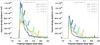 |
Fig. 8 Plasma column density as a function of the distance projected on the plane of the sky along the paths 1, calculated from the COR1-A and -B calibrated images, taken from 3:50 UT to 4:05 UT with 5-min time cadence, and by setting an angular distance of the plasma from the POS of the two coronagraphs of θA = + 16° and θB = −24°, respectively. The arrows with the same colors as the profiles considered approximately indicate the CME front at different times. |
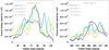 |
Fig. 9 Plasma column density as a function of the position angle along the paths 2, measured counterclockwise from the north pole, at the same times as considered in Fig. 8. The column density are calculated from the COR1-A and -B calibrated images, as described in the caption of Fig. 8. |
3.3. Evidence of plasma depletion in the outer corona
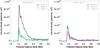 |
Fig. 10 Plasma column density as a function of the distance projected onto the plane of the sky along the paths 1, calculated from the COR1-A and -B calibrated images, taken at 3:40 UT, 18:00 UT, 23:55 UT and at 3:40 UT, 4:45 UT, 18:00 UT, respectively. The computation was made by setting an angular distance of the plasma from the POS of both coronagraphs of 0°. |
The STEREO/COR1 images obtained before the CME event show a highly structured corona. In particular, a faint and short streamer is visible in the portion of the COR1-A FOV that is subsequently affected by the CME, as indicated by the arrow in the top-left panel of Fig. 5. The streamer is brighter than the surrounding corona by a factor of only 2–3 and it is not visible in the FOV of COR1-B.
Following the eruptive event, across the outer coronal area where the CME propagates, a brightness decrease with respect to the early quiescent condition occurs in the COR1 images of both STEREO spacecraft, as a result of the plasma ejection. The observations show that the phenomenon is more evident in the COR1-A images, where the preexisting magnetic structure is not restored within the observational time and the streamer disappears.
We investigated the brightness decrease by also using the results previously obtained, such as location relative to the solar disk, angular width, speed, and column density of the considered CME. We newly computed of the column density, without considering the propagation direction of the CME and setting the angular distance of the ejected plasma at 0° from the POS of both spacecraft, as input to the scc_calc_cme_mass.pro routine. Figure 10 shows the column density profiles along the paths 1 (see Fig. 5), at 3:40 UT (a few minutes before the CME start) and at two subsequent times. The gap in the COR1-A data does not allow us to investigate the coronal restructuring with the STEREO Ahead observations from 4:05 UT to 18:00 UT.
The stereoscopic view provided by the STEREO satellites allows us to accurately analyse the processes at play without missing substantial details, as occurred in the past with observations by a single coronagraph. As described above, the CME propagation results in a brightness decrease in the COR1 images: this is due to a plasma depletion, as indicated by the column density profiles of Fig. 10; but the two plots sketched here, representing observations from the two STEREO viewpoints, show a different scenario. The column density values at 3:40 UT in the COR1-A plot are more than twice as high as those reported in the COR1-B plot at the same time, owing to the presence of the streamer in the relevant COR1-A image. The COR1-B plot shows that a density reduction by a factor of 2 occurs at 4:45 UT and that the early condition (3:40 UT) appears to be totally restored at 18:00 UT. Conversely, the column density profile at 18:00 UT in the COR1-A plot shows values that are a factor of about 3 lower than those pre-CME, confirming the disappearance of the streamer; this last condition is just slightly modified until 23:55 UT, when the column density values are still one third of the pre-event values. All this permits us to conclude that 1) the plasma depletion is highest about one hour after the beginning of the event; 2) the COR1-A observations show a coronal restructuring after the CME; and 3) the COR1-B data indicate a lifetime of the depletion phenomenon shorter than 14 h.
4. Discussion and conclusions
We investigated the restructuring of the outer solar corona produced by the halo CME on 9 March 2012. We used observations from different viewpoints, such as those provided by SOHO, STEREO, and SDO satellites, to investigate the spatial configuration of the CME and determine its direction and speed of propagation. We adopted the polarization ratio technique (e.g. Moran & Davila 2004; Mierla et al. 2009) and applied it to the COR1 data. This technique allowed us to obtain a weighted mean angular distance θ of the ejected plasma from the POS of the spacecraft; but when only a coronagraph is used, the method gives no information about the depth extent of the CME along the LOS. The polarization ratio technique also suffers from an ambiguity caused by the forward/backward symmetry of the Thomson scattering. In spite of these limitations, we were able to determine that the CME moved in the COR1 FOV with an average speed of about 1000 km s-1 and to reconstruct the boundaries of the CME emission distribution, which range from −6° to 36° in heliographic longitude and over about 80° in heliographic latitude. For our computation, we exploited the stereoscopic view provided by the STEREO coronagraphs; moreover, we solved the geometric ambiguity using AIA and LASCO/C2 observations: the former gave us the starting time and position of the CME on the solar disk, while the latter provided one more point of view on how the event moved throughout the corona.
We also estimated the mass of the CME using the COR1 calibrated images in the time interval 3:50–4:05 UT. We obtained values of the CME mass up to 2.2 × 10¹⁶ g, similar to the highest values of mass determined previously (e.g. Hundhausen et al. 1994; Howard et al. 2003).
Before the STEREO mission, studying the influence of CMEs on the coronal structures, such as the preexisting streamers, was limited by the two-dimensionality of the observations. In this scenario, Low (1996) suggested that CMEs arise from flux ropes embedded in a streamer, erupting and disrupting the streamer itself. Conversely, Subramanian et al. (1999) analysed LASCO coronagraphic images and synoptic maps and found that approximately 35% of the CMEs observed from January 1996 to June 1998 seem to have no relation to the preexisting streamer, while 46% have no effect on the streamer, even though they appear to be related to it. The authors attempted to explain the results for these CMEs as owing to their longitudinal displacement from the observed streamer and from the plane of the sky. In this paper we exploited the stereoscopic observations of the corona also to study the effects of the CME on 9 March 2012 on a faint (by a factor of just 2–3 brighter than the surrounding corona) and short streamer, which was only visible in the coronal sector of the FOV of COR1-A coronagraph involved in the passage of the CME. Our results allowed us to deduce that the streamer was located in the same region where the CME propagated and was disrupted by this event.
The very recent results provided by Schrijver & Title (2011) suggested that brightness decrease phenomena in the low and outer corona, namely coronal dimming and plasma depletion, respectively, are more common than expected. However, measurements of the mass loss associated with these events are rare. Therefore, we investigated the brightness decrease that occurred in the coronal sector where the CME propagates, using some characteristics of the CME, such as location relative to the solar disk, angular width, and speed. To provide a further contribution to the study of the investigated phenomena, we also calculated values of column densities before, during, and after the CME event. From the profiles of these column densities, computed along two radial paths at 73° and 290° PA, measured counterclockwise from the north pole in the FOV of COR1-A and -B, respectively, we found a confirmation that the brightness decrease is due to a plasma depletion that was highest at about one hour after the beginning of the CME. Moreover, the combined analysis performed by the two COR1 coronagraphs allowed us to study in more detail the effects of the passage of the CME on the solar corona structure: from the COR1-A observations we verified a coronal reconfiguration after the CME, while from the COR1-B data the plasma depletion appears to have a lifetime shorter than 14 hours.
Note that the synergy among multiple observations was necessary to highlight all phenomena studied in this paper. In this regard, we evaluated the plasma depletion by using the column density data obtained by the two COR1 coronagraphs separately.
First we used the COR1-B data and computed the integral I1 of the difference of the column density values before (3:40 UT) and one hour after (4:45 UT) the beginning of the CME between 1.5 and 2.5 R⊙ over the radial path at 290° PA (see right panel of Fig. 10); then, we computed the integral I2 of the column density at 4:05 UT over the same path (see right panel of Fig. 8), that is, when the CME was totally developed in the FOV of COR1-B. Finally, we calculated the ratio I1/I2, approximately representing the ratio between the mass depletion in the corona and the mass expelled during the CME eruption. This ratio is equal to (1.05 × 1027 electrons cm-1)/(1.45 × 1028 electrons cm-1) ≃ 7%, which is about a factor of 2 higher than the mass ratio obtained by Ramesh & Sastry (2000). They carried out a comparison of radio and white-light observations of the plasma depletion that occurred in the aftermath of a CME event. These authors found a lifetime of the depletion phenomenon shorter than 24 h; in addition, they estimated that the mass expelled during the eruption was about 1.3 × 10¹⁵ g and the coronal mass loss associated with the depletion was about 4.7 × 10¹³ g, which is 4% of the previous value.
Then we used the COR1-A data and calculated the integral I3 of the difference of the column density values at 3:40 UT and at 23:55 UT (when the event was reasonably over) between 1.5 and 2.5 R⊙ over the radial path at 73° PA (see left panel of Fig. 10), and the integral I4 of the column density at 4:05 UT over the same path (when the CME reached its maximum development in the FOV of COR1-A, see left panel of Fig. 8). We found that the ratio I3/I4, with the same meaning as I1/I2, is equal to (1.46 × 1028 electrons cm-1)/(3.01 × 1028 electrons cm-1), which is about 48%. This indicates the disappearance of the preexisting streamer and that its mass, carried away from the concerned coronal area, corresponds to about half of the CME mass. We concluded that the passage of the halo CME significantly affects the coronal structures and the plasma distribution in the area involved in the eruption.
It is here our intention to stress the importance of the synergy among various observational instruments in studying solar
activity. To realize the analysis described in this paper, for instance, the stereoscopic view provided by the STEREO satellites would not have been enough and, in addition, we needed to also exploit the images provided by AIA and LASCO/C2. Systematic observations of the solar corona, carried out in synergy among different instruments, are expected to shed light on the role played by CMEs on the coronal restructuring after the events. These investigations will probably also show possible dependences of the depletion phenomenon or/and streamer disappearance on the CME main characteristics, such as propagation direction, angular width, location relative to the solar disk, speed, and column density.
Online material
Movie of Fig. 3 Access here
Acknowledgments
The authors thank the referee for helpful comments, which led to a sounder version of the paper. This work was partly supported by the Agenzia Spaziale Italiana through contract ASI/INAF No. I/013/12/0 and by the European Commissions Seventh Framework Programme under grant agreements No. 284461 (eHEROES project) and No. 312495 (SOLARNET project). The STEREO/SECCHI data are produced by an international consortium of the NRL, LMSAL and NASA GSFC (USA), RAL and University of Bham (UK), MPS (Germany), CSL (Belgium), and IOTA and IAS (France).
References
- Billings, D. E. 1966, A guide to the Solar Corona (New York: Academic Press) [Google Scholar]
- Brueckner, G. E., Howard, R. A., Koomen, M. J., et al. 1995, Sol. Phys., 162, 357 [NASA ADS] [CrossRef] [Google Scholar]
- Harrison, R. A., & Lyons, M. 2000, A&A, 358, 1097 [NASA ADS] [Google Scholar]
- Harrison, R. A., Harra, L. K., Brković, A., & Parnell, C. E. 2003, A&A, 409, 755 [NASA ADS] [CrossRef] [EDP Sciences] [Google Scholar]
- Howard, R. A., Morrill, J., Vourlidas, A., et al. 2003, AGU Fall Meeting, abstract B460 [Google Scholar]
- Hudson, H. S., & Webb, D. F. 1997, Geophys. Monogr., 99, 27 [Google Scholar]
- Hundhausen, A. J., Stanger, A. L., & Serbicki, S. A. 1994, ESA, 373, 409 [Google Scholar]
- Kaiser, M. L., Kucera, T. A., Davila, J. M., et al. 2008, Space Sci. Rev., 136, 5 [NASA ADS] [CrossRef] [Google Scholar]
- Lemen, J. R., Title, A. M., Akin, D. J., et al. 2012, Sol. Phys., 275, 17 [NASA ADS] [CrossRef] [Google Scholar]
- Liu, Y., Luhmann, J. G., Lin, R. P., et al. 2009, ApJ, 698, 51 [NASA ADS] [CrossRef] [Google Scholar]
- Low, B. C. 1996, Sol. Phys., 167, 217 [Google Scholar]
- Low, B. C. 1997, Geophys. Monogr., 99, 39 [Google Scholar]
- Low, B. C. 2001, J. Geophys. Res., 106, 25141 [NASA ADS] [CrossRef] [Google Scholar]
- Mierla, M., Inhester, B., Marqué, C., et al. 2009, Sol. Phys., 259, 123 [NASA ADS] [CrossRef] [Google Scholar]
- Minnaert, M. 1930, Z. Astrophys., 1, 209 [NASA ADS] [Google Scholar]
- Moran, T. G., & Davila, J. M. 2004, Science, 305, 66 [NASA ADS] [CrossRef] [PubMed] [Google Scholar]
- Ramesh, R., & Sastry, Ch. V. 2000, A&A, 358, 749 [NASA ADS] [Google Scholar]
- Schrijver, C. J., & Title, A. M. 2011, J. Geophys. Res., 116, A04108 [Google Scholar]
- Sime, D. G. 1989, J. Geophys. Res., 94, 151 [NASA ADS] [CrossRef] [Google Scholar]
- Sterling, A. C., & Hudson, H. S. 1997, ApJ, 491, 55 [Google Scholar]
- Subramanian, P., Dere, K. P., Rich, N. B., & Howard, R. A. 1999, J. Geophys. Res., 104, 22321 [NASA ADS] [CrossRef] [Google Scholar]
- Thompson, W. T., & Reginald, N. L. 2008, Sol. Phys., 250, 443 [NASA ADS] [CrossRef] [Google Scholar]
- Thompson, B. J., Cliver, E. W., Nitta, N., Delannée, C., & Delaboudinière, J.-P. 2000, Geophys. Res. Lett., 27, 1431 [Google Scholar]
- Van De Hulst, H. C. 1950, Bull. Astron. Inst. Netherland, 410, 135 [Google Scholar]
- Webb, D. F., Cliver, E. W., Crooker, N. U., St Cyr, O. C., & Thompson, B. J. 2000, J. Geophys. Res., 105, 7491 [Google Scholar]
All Tables
CME mass values in grams calculated at different times, corresponding to the four COR1 observations in the time interval 3:50–4:05 UT.
All Figures
|
Fig. 1 LASCO/C2 image at 4:50 UT on 9 March 2012. The white circle outlines the limb of the solar disk. |
| In the text | |
|
Fig. 2 GOES X-ray (1–8 Å) emission from 0:00 UT to 8:00 UT on 9 March 2012. The flare onset (~3:25 UT) corresponds to the rapid flux increase. The red vertical line indicates the time of the peak of the flare (3:53 UT), while the black vertical line coincides with the beginning of the LASCO/C2 observation of the CME (4:26 UT). |
| In the text | |
|
Fig. 3 SDO/AIA 193 Å image at 3:42 UT on 9 March 2012. The arrow points out active region NOAA 11429. An animation showing the coronal wave by running difference images is available online. |
| In the text | |
|
Fig. 4 Positions of the STEREO Ahead (red) and Behind (blue) spacecrafts relative to the Sun (yellow) and Earth (green) on 9 March 2012. Distances are in astronomical units in a Cartesian heliocentric Earth ecliptic (HEE) coordinate system. |
| In the text | |
|
Fig. 5 STEREO/COR1 Ahead (left) and Behind (right) images at 3:40 UT (before the CME, top panels) and at 4:00 UT (during the CME, bottom panels). The arrow in the image of the top-left panel points at a faint and short streamer visible in the FOV of COR1-A, before the CME propagation. In the images of the bottom panels, paths 1 are along a radial direction at 73° and 290° PA (measured counterclockwise from North) in the FOV of COR1-A and COR1-B, while paths 2 are perpendicular to the respective paths 1 and extend from 42° to 104° PA and from 257° to 323° PA in the FOV of COR1-A and COR1-B. |
| In the text | |
|
Fig. 6 Sun-STEREO satellites and Sun-Earth directions (short-dashed lines), the STEREO-A POS direction (long-dashed line) and the north polar view of the LASCO/C2 occulter (solid line). The solid blue lines indicate the two possible propagation directions of the ejected plasma at the mean angular distances θA and |
| In the text | |
|
Fig. 7 3D reconstruction of the CME, obtained by the polarization ratio technique applied to the COR1-A and -B data at 4:00 UT. The gray sphere represents the Sun. The numbers on the sphere are the values of HEEQ longitudes, where the X-axis points towards the Earth. The radius of the outer gridded sphere is 1.4 R⊙. |
| In the text | |
|
Fig. 8 Plasma column density as a function of the distance projected on the plane of the sky along the paths 1, calculated from the COR1-A and -B calibrated images, taken from 3:50 UT to 4:05 UT with 5-min time cadence, and by setting an angular distance of the plasma from the POS of the two coronagraphs of θA = + 16° and θB = −24°, respectively. The arrows with the same colors as the profiles considered approximately indicate the CME front at different times. |
| In the text | |
|
Fig. 9 Plasma column density as a function of the position angle along the paths 2, measured counterclockwise from the north pole, at the same times as considered in Fig. 8. The column density are calculated from the COR1-A and -B calibrated images, as described in the caption of Fig. 8. |
| In the text | |
|
Fig. 10 Plasma column density as a function of the distance projected onto the plane of the sky along the paths 1, calculated from the COR1-A and -B calibrated images, taken at 3:40 UT, 18:00 UT, 23:55 UT and at 3:40 UT, 4:45 UT, 18:00 UT, respectively. The computation was made by setting an angular distance of the plasma from the POS of both coronagraphs of 0°. |
| In the text | |
Current usage metrics show cumulative count of Article Views (full-text article views including HTML views, PDF and ePub downloads, according to the available data) and Abstracts Views on Vision4Press platform.
Data correspond to usage on the plateform after 2015. The current usage metrics is available 48-96 hours after online publication and is updated daily on week days.
Initial download of the metrics may take a while.