| Issue |
A&A
Volume 566, June 2014
|
|
|---|---|---|
| Article Number | A3 | |
| Number of page(s) | 18 | |
| Section | Stellar atmospheres | |
| DOI | https://doi.org/10.1051/0004-6361/201423711 | |
| Published online | 29 May 2014 | |
The virtual observatory service TheoSSA: Establishing a database of synthetic stellar flux standards
II. NLTE spectral analysis of the OB-type subdwarf Feige 110⋆,⋆⋆,⋆⋆⋆
1 Institute for Astronomy and Astrophysics, Kepler Center for Astro and Particle Physics, Eberhard Karls University, Sand 1, 72076 Tübingen, Germany
e-mail: This email address is being protected from spambots. You need JavaScript enabled to view it.
2 NASA Goddard Space Flight Center, Greenbelt MD 20771, USA
3 European Southern Observatory, Karl-Schwarzschild-Str. 2, 85748 Garching, Germany
Received: 26 February 2014
Accepted: 8 April 2014
Abstract
Context. In the framework of the Virtual Observatory (VO), the German Astrophysical VO (GAVO) developed the registered service TheoSSA (Theoretical Stellar Spectra Access). It provides easy access to stellar spectral energy distributions (SEDs) and is intended to ingest SEDs calculated by any model-atmosphere code, generally for all effective temperatures, surface gravities, and elemental compositions. We will establish a database of SEDs of flux standards that are easily accessible via TheoSSA’s web interface.
Aims. The OB-type subdwarf Feige 110 is a standard star for flux calibration. State-of-the-art non-local thermodynamic equilibrium stellar-atmosphere models that consider opacities of species up to trans-iron elements will be used to provide a reliable synthetic spectrum to compare with observations.
Methods. In case of Feige 110, we demonstrate that the model reproduces not only its overall continuum shape from the far-ultraviolet (FUV) to the optical wavelength range but also the numerous metal lines exhibited in its FUV spectrum.
Results. We present a state-of-the-art spectral analysis of Feige 110. We determined , log g = 6.00 ± 0.20, and the abundances of He, N, P, S, Ti, V, Cr, Mn, Fe, Co, Ni, Zn, and Ge. Ti, V, Mn, Co, Zn, and Ge were identified for the first time in this star. Upper abundance limits were derived for C, O, Si, Ca, and Sc.
Conclusions. The TheoSSA database of theoretical SEDs of stellar flux standards guarantees that the flux calibration of astronomical data and cross-calibration between different instruments can be based on models and SEDs calculated with state-of-the-art model-atmosphere codes.
Key words: standards / stars: abundances / stars: atmospheres / stars: individual: Feige 110 / subdwarfs / virtual observatory tools
Based on observations with the NASA/ESA Hubble Space Telescope, obtained at the Space Telescope Science Institute, which is operated by the Association of Universities for Research in Astronomy, Inc., under NASA contract NAS5-26666.
Based on observations made with the NASA-CNES-CSA Far Ultraviolet Spectroscopic Explorer.
Table 2, Figs. 3 and 7 are available in electronic form at http://www.aanda.org
© ESO, 2014
1. Introduction
Feige 110 is a bright (mV = 11.845 ± 0.010, Kharchenko & Roeser 2009), subluminous OB-star (type sdOB, Heber et al. 1984a; type sdO D,Vennes et al. 2011). It is widely used as a spectrophotometric standard star (e.g. Oke 1990; Turnshek et al. 1990; Bohlin et al. 1990). Since Feige 110 will be used as a reference star for the flux calibration of X-Shooter1 (Vernet et al. 2011) observations from 3000 Å to 25 000 Å (Moehler et al. 2014), we decided to reanalyze its spectrum with state-of-the-art model-atmosphere techniques.
An early spectral analysis with approximate LTE2, line-blanketed hydrogen model atmospheres yielded an effective temperature and a surface gravity log (g/ cm/s2) = 6.5 (Newell 1973). Kudritzki (1976) showed that both, the consideration of deviations from non-LTE (NLTE) as well as of opacities of elements heavier than H, have a significant influence on the determination of Teff and log g in an analysis of optical spectra (Table 1). Heber et al. (1984a) extended the analysis of Feige 110 to the ultraviolet (UV) wavelength range (IUE3 observations, 1150 Å ≲ λ ≲ 2000 Å) in addition to high-resolution optical spectra (4000 Å ≲ λ ≲ 5100 Å) and derived , log g = 5.0 ± 0.3, and He/H = 0.03 (by number) using H+He (with subsequent C+N+Si line-formation calculations) NLTE models.
Teff and log g of Feige 110 determined by Kudritzki (1976).
With the FUSE4 mission, the interstellar deuterium and oxygen column densities toward Feige 110 were measured. Friedman et al. (2002) used optical spectra and estimated the atmospheric parameters by comparison with a grid of synthetic NLTE model-atmosphere spectra (using TLUSTY to compute the stellar atmosphere model and SYNSPEC to generate the SED, Hubeny & Lanz 1995, just “TLUSTY” hereafter), that considered H and He. They achieved , log g = 5.95 ± 0.15, and He/H = 0.011 ± 0.005. With the higher log g (in agreement with Kudritzki 1976), their spectroscopic distance of d = 288 ± 43 pc agreed with the Hipparcos5 parallax distance of  .
.
In the following, we describe our analysis in detail. In Sect. 2, we give some remarks on the observations. Then, we introduce our models and the considered atomic data (Sect. 3) and start with a preliminary analysis (Sect. 4) of the optical spectrum based on H+He models followed by a highly sophisticated analysis with metal-line blanketed models (Sect. 5). We summarize our results and conclude in Sect. 6.
2. Observations
Our main optical spectrum is a median of 19 X-Shooter observations, taken between 26 October 2011 and 5 July 2012 with a 5″ slit (the seeing was below 1″ during the observations) and an exposure time of 120 s each. The achieved resolving power was R = λ/ Δλ ≈ 4800. All spectra were extracted with ESO’s standard pipeline-reduction software (with the actual version at the time of the respective observation). Heliocentric correction and correction to an airmass =0 were applied. In addition, we used optical HST/STIS6 spectra (ObsIds O40801010 and O40801030 co-added) from the archive for the determination of the interstellar reddening.
Our far-ultraviolet (FUV) spectrum consists of two observations of Feige 110 that were performed by FUSE, both in June 2000 and both through the LWRS spectrograph aperture. The dataset IDs were M1080801 and P1044301, with exposure times of 6.2 ks and 21.8 ks, respectively. Alignment of the four FUSE telescope channels was excellent throughout both observations, with RMS exposure-to-exposure variations in flux under 0.5% in all channels. The processing of individual exposures to produce a combined spectrum spanning 905–1188Å was the same as that described for G191−B2B in Rauch et al. (2013) and won’t be repeated here. The signal to noise per 0.013 Å pixel in the continuum for the combined spectrum is typically 80:1 shortward of 1000 Å and 120:1 longward of 1000 Å. Approximately 37% of the exposure time was obtained during orbital night. Comparison of the spectra obtained during day and night portions of the orbit found a discernible difference only in the cores of Ly β and Ly γ. Only the night data were used for these spectral regions. Weak airglow emission was still present at Ly β during orbital night, but the affected pixels had no impact on the analysis of the stellar spectrum.
Additional UV spectra were retrieved from MAST. We used all available low-resolution IUE spectra (SWP03737, SWP20091, SWP21888, SWP21890, SWP21891, SWP21892, LWP01913, LWP01914, LWP01915, LWP02505, LWP02506, LWP02507, LWP02508, and LWR11785 co-added) and an HST/STIS spectrum (ObsId OBIE01010, exposure time 1734.2 s, start time 2010-12-12 08:10:54 UT, grating G140M, 1191 Å ≲ λ ≲ 1246 Å, aperture  , resolution = 0.1 Å).
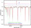 |
Fig. 1 Comparison of three synthetic spectra with our optical observation of Feige 110. Teff , log g , and the H:He ratio by mass are indicated. |
3. Model atmospheres and atomic data
For our model-atmosphere calculations, we use the Tübingen NLTE model-atmosphere package7 (Werner et al. 2003; Rauch & Deetjen 2003), that assumes a plane-parallel geometry and considers opacities of elements from H to Ni (Rauch 1997, 2003). The models are in hydrostatic and radiative equilibrium. TMAP was successfully used for many spectral analyses of hot, compact stars (e.g. Rauch et al. 2007, 2013; Wassermann et al. 2010; Klepp & Rauch 2011; Ziegler et al. 2012).
The model atoms used in our model-atmosphere calculations were either retrieved from the Tübingen model-atom database8 or compiled via the registered Virtual Observatory (VO) tool TIRO9 that uses Kurucz’s atomic data10 and line lists (Kurucz 1991, 2009, 2011, and priv. comm.). Table 2 shows the statistics of our model atoms.
4. Preliminary analysis
For a preliminary analysis, or verification of basic previous results, we employ the registered VO service TheoSSA11 and the related registered VO tool TMAW12, to download pre-calculated synthetic spectral energy distributions (SEDs) or to calculate individual SEDs, respectively (cf. Rauch et al. 2013). Figure 1 shows a comparison of SEDs with model parameters of Heber et al. (1984a), Friedman et al. (2002), and of this work with the observed optical spectrum. The Balmer decrement is a sensitive indicator of log g (e.g. Rauch et al. 1998), and we derive log g = 5.90 ± 0.20. At this log g , the He i/He ii ionization equilibrium, i.e. the measured equivalent-width ratio of He i and He ii lines, is well reproduced by our model at . The He line strengths are matched at a photospheric He abundance of 8 ± 2% by mass. Although the theoretical H and He line profiles agree well with the observation, the central depressions are not matched perfectly. This may be a hint that a weak Balmer-line problem (cf. Napiwotzki & Rauch 1994; Rauch 2000) exists because metal opacities are neglected. For the same reason, our synthetic H+He SEDs are not suitable for an analysis of the H i Lyman lines in FUV spectrum. Fully metal-line blanketed model-atmospheres are mandatory for this purpose (Sect. 5). However, from our derived Teff , we are well in the parameter range where no deviation between H i Lyman- and Balmer-line analysis is expected (Good et al. 2004, their Fig. 4).
We adopt our derived Teff and log g values, that also reproduce well the HST/STIS observation (Fig. 2), for our further analysis and will verify them with our final, fully metal-line blanketed model.
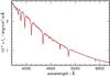 |
Fig. 2 Comparison of the optical HST/STIS observation with our final model SED. The synthetic spectrum is convolved with a Gaussian (FWHM = 5 Å) to match the resolution of the observation. The error bar indicates the visual brightness (mV = 11.847 ± 0.010). |
Within error limits, our preliminary values agree well with those of Friedman et al. (2002). Only ΔTeff = ± 1000 from their χ2 fit appears to be too optimistic. It is worthwhile to note, that the result of Kudritzki (1976, Table 1, his lower He abundance model) is relatively close to our result.
5. Line identification and detailed analysis
Friedman et al. (2002) identified photospheric lines from N iii–v, S vi, Cr iv–v, Fe iii–iv, and Ni iv in the FUSE observation. Their SED calculation (SYNSPEC, Hubeny & Lanz 1995) included all elements from H to Zn, all with solar abundances but He (1.3 × 10⁻¹ times solar), C (≈4 × 10⁻⁶ times solar), Si (≈2 × 10⁻⁷ times solar), and Cr (≈21 times solar).
We decided to include H, He, C, N, O, Si, P, S, Ca, Sc, Ti, V, Cr, Mn, Fe, Co, Ni, Zn, and Ge in our calculations. Figure 3 shows the ionization fractions of these elements. For the iron-group elements (here Ca–Ni), the dominant ionization stages are iv–v. All SEDs that were calculated for this analysis are available via TheoSSA.
For the line identification in the FUSE wavelength range (905–1188 Å), it was necessary to determine the stellar continuum flux precisely. We started with a measurement of the interstellar neutral hydrogen column density. From Ly α in the STIS spectrum and the higher members of the Lyman series in the FUSE spectrum, we determined nH i = 1.8 ± 0.8 × 1020 cm-2 in agreement with Friedman et al. (2002, nH i = 1.4 ± 0.5 × 1020 cm-2. To measure the interstellar reddening, we normalized our synthetic spectrum to the 2MASS H brightness because the interstellar reddening is negligible there and adjusted EB − V to match the IUE, STIS, and FUSE flux levels. Our result is EB − V = 0.027 ± 0.007. This very low value is in agreement with the absence of the 2175 Å bump in the IUE LWP spectra (Sect. 2). The Galactic reddening law of Liszt (2014a,b, valid for 0.015 ≲ EB − V ≲ 0.075 and | b | ≥ 20°, NH i/EB − V = 8.3 × 1021 cm-2mag-1, predicts 0.012 ≤ EB − V ≤ 0.031 in agreement with our value.
The comparison of our models to the FUSE observations shows that we can reproduce well the observed flux level (Fig. 4), if we include all the lines from Kurucz’s LIN lists (Sect. 3). These include laboratory-measured lines with “good wavelengths” as well as theoretical lines13. The lines with good wavelengths are presented in Kurucz’s POS lists. Unfortunately, the ratio of LIN to POS lines is about 100 and thus, most line wavelengths are uncertain. Moreover, the continuum flux of the POS-line spectrum appears artificially high compared to the LIN spectrum due to the neglected line opacity (Fig. 5).
The line-identification process is easy (the comparison of two SEDs calculated from our final model where the oscillator strengths of one individual atom/ion was artificially reduced for one SED). It enabled us to unambiguously identify hundreds of lines of N, O, P, S, Ti, V, Cr, Mn, Fe, Mn, Ni, Zn, and Ge.
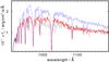 |
Fig. 4 FUSE observation of Feige 110 (gray) compared with two synthetic spectra calculated from our final model (thin, blue in the online version: with Kurucz’s POS lines; thick, red: with Kurucz’s LIN lines). All spectra are convolved with a Gaussian (FWHM = 1 Å) for clarity. |
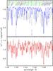 |
Fig. 5 Same as Fig. 4, for a section of the FUSE observation (top panel: POS, bottom panel: LIN). The POS lines are identified (in black, Fe and Ni lines in blue and green for clarity, respectively) at the top of the top panel. Lines of interstellar origin are marked in blue (with subscript “is”) at the bottom of the top panel. The synthetic spectra are convolved with a Gaussian (FWHM = 0.06 Å) to match FUSE’s resolution. |
Our metal-line blanketed models have a different atmospheric structure compared to the H-He models that were used in the preliminary determination of and log g = 5.90 (Sect. 4). Figure 6 shows the typical surface-cooling (log m ≲ –2.5) and backwarming effects (log m ≳ − 2.5), that are an impact of the additionally considered metal opacities. A detailed evaluation of the optical spectrum shows that slightly higher and log g = 6.00 values are necessary to reproduce the He i/He ii ionization equilibrium and the observed H i, He i, and He ii line profiles best.
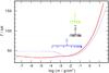 |
Fig. 6 Temperature structure of our H+He model (thin, blue line: , log g = 5.90), a metal-line blanketed model with the same Teff and log g (dashed, red), and of our final model (thick, red: , log g = 6.00). The formation depths of the lines cores of optical lines of H i (H α is the most outside), He i, and He ii are shown. |
The abundance analysis follows a standard procedure. Identified lines are reproduced by an abundance adjustment of the respective species. For elements with no lines identified, we increased the abundances until their line-detection limit. The optical spectrum was used to further constrain the upper limit because lines of lower ionization stages, that are not observed, appear there at too-high abundances in the synthetic spectrum. Table 3 summarizes the lines that were used and the derived abundances.
Strategic lines and determined element abundances (mass fraction, error ± 0.2 dex).
To identify ISM14 absorption lines in the FUSE observation (cf. Friedman et al. 2002) and to judge the contamination of photospheric lines, we follow our standard procedure and model the stellar spectrum simultaneously with the ISM line absorption (e.g., Rauch et al. 2013). We modeled the latter with the program OWENS (Hébrard et al. 2002; Hébrard & Moos 2003), that considers different clouds with individual radial and turbulent velocities, temperatures, column densities and chemical compositions. Lines are represented by Voigt profiles. The best fit is determined via a χ2 method. Our ISM model includes lines of H2 (J = 0–9), H i, D i, C ii–iii, N i–ii, O i, Si i–ii, P ii, Ar i, and Fe ii. Our results for D i and O i are consistent with those of Friedman et al. (2002).
The complete FUSE observation is compared (including line identifications) with our final model in Fig. 7.
6. Results and conclusions
We performed a comprehensive spectral analysis of Feige 110, based on observations from the FUV to the optical wavelength range. We determined and log g = 6.00 ± 0.20. The ionization equilibria of He i/He ii, N iii/N iv/N v, P iv/P v, S iv/S v/S vi, Ti iv/Ti v, V iv/V v, Cr iv/Cr v/Cr vi, Mn v/Mn vi, Fe v/Fe vi, Co v/Co vi, and Ni v/Ni vi are well reproduced with these values. The photospheric abundances were determined based on the FUSE and optical observations (Table 3). Figure 8 shows a comparison of the photospheric abundances patterns of three hot O(B)-type subdwarfs. While the intermediate-mass metals are solar or subsolar in all these stars, the iron-group elements but Fe have strongly super-solar values. An exception is Fe in AA Dor and EC 11481−2303, that appears to be solar. Neither this Fe peculiarity nor the extremely low C and Si abundances in Feige 110 can be explained.
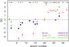 |
Fig. 8 Comparison of the determined photospheric abundances (arrows indicate upper limits) of the three OB-type subdwarfs AA Dor (Klepp & Rauch 2011), EC 11481−2303 (Rauch et al. 2010), and Feige 110. Their Teff and log g are shown in the legend. |
The position of Feige 110 in the Teff −log g plane shows that it is located directly on the He main sequence (Fig. 9). Feige 110 belongs, like AA Dor or EC 11481−2303, to the hottest post-EHB15 stars. From a comparison to post-EHB tracks (Dorman et al. 1993), we can extrapolate a stellar mass of M = 0.469 ± 0.001 M⊙. With  (G is the gravitational constant), we calculated the stellar radius of
  .
.
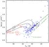 |
Fig. 9 Location of Feige 110 in the Teff −log g plane compared to sdBs and sdOBs from Edelmann (2003), Rauch et al. (2010, EC 11481−2303, and Klepp & Rauch (2011, AA Dor. Post-EHB tracks from Dorman et al. (1993, YHB = 0.288, labeled with the respective stellar masses in M⊙ are also shown. Their start and kink points are used to illustrate the location of the zero-age and terminal-age EHB for this He composition. The He main sequence is taken from Paczyński (1971). |
We determined the distance of Feige 110 following the flux calibration of Heber et al. (1984b) for λeff = 5454 Å,  (1)with mVo = mV − 2.175c, c = 1.475EB − V, and the Eddington flux Hν = 7.24 ± 0.37 × 10⁻⁴ erg/cm2/ s/Hz at λeff of our final model atmosphere. We used EB − V = 0.027 ± 0.007 (Sect. 4), M = 0.469 ± + 0.001 M⊙, and mV = 11.847 ± 0.010 (Kharchenko & Roeser 2009) and derived a distance of
  pc and a height below the Galactic plane of
  pc. This distance is about a factor of three larger than the new Hipparcos parallax-measurement reduction (van Leeuwen 2007, HIP115195, π = 9.76 ± 3.44 mas) of
  pc. Interestingly, the older Hipparcos measurement published by Perryman et al. (1997, π = 5.59 ± 3.34 mas,
  deviates from this new value by a factor of almost two and would be in agreement with our spectroscopic distance within error limits.
The discrepancy between spectroscopic and parallax distances is a significant problem. log g cannot be higher by about 0.5 to achieve a distance agreement, because the spectral lines in the models appear too broad and too shallow. This apparently is not a problem of our TMAP code, because Friedman et al. (2002, dspec = 288 ± 43 used the TLUSTY code and encountered the same problem. Similar discrepancies are reported by Rauch et al. (2007, for LSV+46°21 with TMAP:  vs.
vs.  and by Latour et al. (2013, for BD+28°4211 with TLUSTY, , log g = 6.2, and an assumed M = 0.5 M⊙: dspec = 157 pc
 .
.
Latour et al. (2013) mentioned that a relatively high log g value and/or a low mass may be the solution and since they regard the Hipparcos measurement as fully reliable and their TLUSTY results reasonably reliable, the mass of BD+28°4211 must be much less than the canonical post-EHB mass of about 0.5 M⊙. For their dparallax/dspec = 0.59, the mass has to be about 0.17 M⊙. In case of Feige 110, with dparallax/dspec = 0.31, the mass has to be about 0.10 M⊙. In both cases, the mass can be higher, if log g is higher. Thus, since log g is also the main error source in the spectroscopic distance (Eq. (1)), one might speculate about the applied broadening theory for lines that are used to determine log g . For the relevant H i and He ii lines (linear Stark effect), TMAP as well as TLUSTY use the same data of Tremblay & Bergeron (2009) and Schöning & Butler (1989), respectively. However, all the narrow metal lines (e.g. of the iron-group element) in the UV, that are broadened by the quadratic Stark effect, cannot be reproduced at a much higher log g . To summarize, the distance discrepancy is as yet unexplained.
The analysis of the FUV spectrum has shown that the lack of reliably measured wavelengths of lines of the iron-group elements (Ca−Ni) and of elements heavier than Ni hampers the line-identification. Efforts in this field in the near future are highly desirable.
The established database of spectrophotometric standard stars in TheoSSA was extended by the OB-type subdwarf Feige 110. The successfully launched Gaia16 mission will provide accurate parallax measurements for spectrophotometric standard stars. This will strengthen the importance of a VO-compliant database like TheoSSA that provides easy access to the best synthetic spectra calculated for these stars.
Online material
Statistics of the atoms used in our calculations.
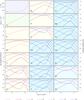 |
Fig. 3 Temperature and density structure and ionizations fractions of our final model with and log g = 6.00; m is the column mass, measured from the outer boundary of our model atmosphere. |
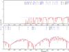 |
Fig. 7 FUSE spectrum of Feige 110 (gray) compared with synthetic spectra calculated from our final model (red: Kurucz’s LIN lines and interstellar line absorption, blue: Kurucz’s POS lines). The locations of the strongest stellar (marked in black, Fe and Ni which have the most lines are marked in blue and green for clarity, respectively, for Ca–Ni, only Kurucz’s POS lines are identified) and interstellar (marked in blue, with subscript “is”) lines are indicated at the top of the panels. The small, green identification marks at the bottom of the panels indicate the locations of interstellar H2 lines. |
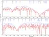 |
Fig. 7 continued. |
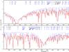 |
Fig. 7 continued. |
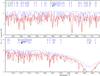 |
Fig. 7 continued. |
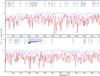 |
Fig. 7 continued. |
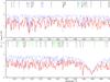 |
Fig. 7 continued. |
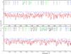 |
Fig. 7 continued. |
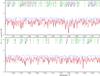 |
Fig. 7 continued. |
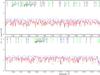 |
Fig. 7 continued. |
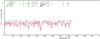 |
Fig. 7 continued. |
Local thermodynamic equilibrium.
International Ultraviolet Explorer.
Far Ultraviolet Spectroscopic Explorer.
Hubble Space Telescope/Space Telescope Imaging Spectrograph.
Tübingen iron-opacity interface.
Theoretical Stellar Spectra Access, http://dc.g-vo.org/theossa
Tübingen Model-Atmosphere WWW Interface.
Kurucz’s LIN lists are used in our model-atmosphere calculations.
Interstellar medium.
Extended horizontal branch.
Acknowledgments
T.R. is supported by the German Aerospace Center (DLR, grant 05 OR 1301). The GAVO project at Tübingen has been supported by the Federal Ministry of Education and Research (BMBF, grants 05 AC 6 VTB, 05 AC 11 VTB). This work used the profile-fitting procedure OWENS developed by M. Lemoine and the FUSE French Team. This research has made use of the SIMBAD database, operated at the CDS, Strasbourg, France. This research has made use of NASA’s Astrophysics Data System. Some of the data presented in this paper were obtained from the Mikulski Archive for Space Telescopes (MAST). STScI is operated by the Association of Universities for Research in Astronomy, Inc., under NASA contract NAS5-26555. Support for MAST for non-HST data is provided by the NASA Office of Space Science via grant NNX09AF08G and by other grants and contracts. The TIRO service (http://astro-uni-tuebingen.de/~TIRO) used to calculate opacities for this paper was constructed as part of the activities of the German Astrophysical Virtual Observatory. The TMAW service (http://astro-uni-tuebingen.de/~TMAW) used to calculate theoretical spectra for this paper was constructed as part of the activities of the German Astrophysical Virtual Observatory.
References
- Asplund, M., Grevesse, N., Sauval, A. J., & Scott, P. 2009, ARA&A, 47, 481 [NASA ADS] [CrossRef] [Google Scholar]
- Bohlin, R. C., Harris, A. W., Holm, A. V., & Gry, C. 1990, ApJS, 73, 413 [NASA ADS] [CrossRef] [Google Scholar]
- Dorman, B., Rood, R. T., & O’Connell, R. W. 1993, ApJ, 419, 596 [CrossRef] [Google Scholar]
- Edelmann, H. 2003, Dissertation, University Erlangen-Nuremberg, Germany [Google Scholar]
- Friedman, S. D., Howk, J. C., Chayer, P., et al. 2002, ApJS, 140, 37 [NASA ADS] [CrossRef] [Google Scholar]
- Good, S. A., Barstow, M. A., Holberg, J. B., et al. 2004, MNRAS, 355, 1031 [NASA ADS] [CrossRef] [Google Scholar]
- Heber, U., Hamann, W.-R., Hunger, K., et al. 1984a, A&A, 136, 331 [NASA ADS] [Google Scholar]
- Heber, U., Hunger, K., Jonas, G., & Kudritzki, R. P. 1984b, A&A, 130, 119 [NASA ADS] [Google Scholar]
- Hébrard, G., & Moos, H. W. 2003, ApJ, 599, 297 [NASA ADS] [CrossRef] [Google Scholar]
- Hébrard, G., Friedman, S. D., Kruk, J. W., et al. 2002, Planet. Space Sci., 50, 1169 [NASA ADS] [CrossRef] [Google Scholar]
- Hubeny, I., & Lanz, T. 1995, ApJ, 439, 875 [Google Scholar]
- Kharchenko, N. V., & Roeser, S. 2009, VizieR Online Data Catalog: I/280 [Google Scholar]
- Klepp, S., & Rauch, T. 2011, A&A, 531, L7 [NASA ADS] [CrossRef] [EDP Sciences] [Google Scholar]
- Kudritzki, R.-P. 1976, A&A, 52, 11 [NASA ADS] [Google Scholar]
- Kurucz, R. L. 1991, in Stellar Atmospheres – Beyond Classical Models, eds. L. Crivellari, I. Hubeny, & D. G. Hummer, NATO ASIC Proc. 341, 441 [Google Scholar]
- Kurucz, R. L. 2009, in AIP Conf. Ser. 1171, eds. I. Hubeny, J. M. Stone, K. MacGregor, & K. Werner, 43 [Google Scholar]
- Kurucz, R. L. 2011, Canadian J. Phys., 89, 417 [NASA ADS] [CrossRef] [Google Scholar]
- Latour, M., Fontaine, G., Chayer, P., & Brassard, P. 2013, ApJ, 773, 84 [NASA ADS] [CrossRef] [Google Scholar]
- Liszt, H. 2014a, ApJ, 783, 17 [NASA ADS] [CrossRef] [Google Scholar]
- Liszt, H. 2014b, ApJ, 780, 10 [NASA ADS] [CrossRef] [Google Scholar]
- Moehler, S., Modigliani, A., Freudling, W., et al. 2014, A&A, in press, DOI: 10.1051/0004-6361/201423790 [Google Scholar]
- Napiwotzki, R., & Rauch, T. 1994, A&A, 285, 603 [NASA ADS] [Google Scholar]
- Newell, E. B. 1973, ApJS, 26, 37 [NASA ADS] [CrossRef] [Google Scholar]
- Oke, J. B. 1990, AJ, 99, 1621 [NASA ADS] [CrossRef] [Google Scholar]
- Paczyński, B. 1971, Acta Astron., 21, 1 [NASA ADS] [Google Scholar]
- Perryman, M. A. C., Lindegren, L., Kovalevsky, J., et al. 1997, A&A, 323, L49 [NASA ADS] [Google Scholar]
- Rauch, T. 1997, A&A, 320, 237 [NASA ADS] [Google Scholar]
- Rauch, T. 2000, A&A, 356, 665 [NASA ADS] [Google Scholar]
- Rauch, T. 2003, A&A, 403, 709 [NASA ADS] [CrossRef] [EDP Sciences] [Google Scholar]
- Rauch, T., & Deetjen, J. L. 2003, in Stellar Atmosphere Modeling, eds. I. Hubeny, D. Mihalas, & K. Werner, ASP Conf. Ser., 288, 103 [Google Scholar]
- Rauch, T., Dreizler, S., & Wolff, B. 1998, A&A, 338, 651 [NASA ADS] [Google Scholar]
- Rauch, T., Ziegler, M., Werner, K., et al. 2007, A&A, 470, 317 [NASA ADS] [CrossRef] [EDP Sciences] [Google Scholar]
- Rauch, T., Werner, K., & Kruk, J. W. 2010, Ap&SS, 329, 133 [NASA ADS] [CrossRef] [Google Scholar]
- Rauch, T., Werner, K., Bohlin, R., & Kruk, J. W. 2013, A&A, 560, A106 [NASA ADS] [CrossRef] [EDP Sciences] [Google Scholar]
- Schöning, T., & Butler, K. 1989, A&AS, 78, 51 [NASA ADS] [Google Scholar]
- Tremblay, P.-E., & Bergeron, P. 2009, ApJ, 696, 1755 [NASA ADS] [CrossRef] [Google Scholar]
- Turnshek, D. A., Bohlin, R. C., Williamson, II, R. L., et al. 1990, AJ, 99, 1243 [NASA ADS] [CrossRef] [Google Scholar]
- van Leeuwen, F. 2007, A&A, 474, 653 [NASA ADS] [CrossRef] [EDP Sciences] [Google Scholar]
- Vennes, S., Kawka, A., & Németh, P. 2011, MNRAS, 410, 2095 [NASA ADS] [Google Scholar]
- Vernet, J., Dekker, H., D’Odorico, S., et al. 2011, A&A, 536, A105 [NASA ADS] [CrossRef] [EDP Sciences] [Google Scholar]
- Wassermann, D., Werner, K., Rauch, T., & Kruk, J. W. 2010, A&A, 524, A9 [NASA ADS] [CrossRef] [EDP Sciences] [Google Scholar]
- Werner, K., Deetjen, J. L., Dreizler, S., et al. 2003, in Stellar Atmosphere Modeling, eds. I. Hubeny, D. Mihalas, & K. Werner, ASP Conf. Ser., 288, 31 [Google Scholar]
- Ziegler, M., Rauch, T., Werner, K., Köppen, J., & Kruk, J. W. 2012, A&A, 548, A109 [NASA ADS] [CrossRef] [EDP Sciences] [Google Scholar]
All Tables
Strategic lines and determined element abundances (mass fraction, error ± 0.2 dex).
All Figures
|
Fig. 1 Comparison of three synthetic spectra with our optical observation of Feige 110. Teff , log g , and the H:He ratio by mass are indicated. |
| In the text | |
|
Fig. 2 Comparison of the optical HST/STIS observation with our final model SED. The synthetic spectrum is convolved with a Gaussian (FWHM = 5 Å) to match the resolution of the observation. The error bar indicates the visual brightness (mV = 11.847 ± 0.010). |
| In the text | |
|
Fig. 4 FUSE observation of Feige 110 (gray) compared with two synthetic spectra calculated from our final model (thin, blue in the online version: with Kurucz’s POS lines; thick, red: with Kurucz’s LIN lines). All spectra are convolved with a Gaussian (FWHM = 1 Å) for clarity. |
| In the text | |
|
Fig. 5 Same as Fig. 4, for a section of the FUSE observation (top panel: POS, bottom panel: LIN). The POS lines are identified (in black, Fe and Ni lines in blue and green for clarity, respectively) at the top of the top panel. Lines of interstellar origin are marked in blue (with subscript “is”) at the bottom of the top panel. The synthetic spectra are convolved with a Gaussian (FWHM = 0.06 Å) to match FUSE’s resolution. |
| In the text | |
|
Fig. 6 Temperature structure of our H+He model (thin, blue line: , log g = 5.90), a metal-line blanketed model with the same Teff and log g (dashed, red), and of our final model (thick, red: , log g = 6.00). The formation depths of the lines cores of optical lines of H i (H α is the most outside), He i, and He ii are shown. |
| In the text | |
|
Fig. 8 Comparison of the determined photospheric abundances (arrows indicate upper limits) of the three OB-type subdwarfs AA Dor (Klepp & Rauch 2011), EC 11481−2303 (Rauch et al. 2010), and Feige 110. Their Teff and log g are shown in the legend. |
| In the text | |
|
Fig. 9 Location of Feige 110 in the Teff −log g plane compared to sdBs and sdOBs from Edelmann (2003), Rauch et al. (2010, EC 11481−2303, and Klepp & Rauch (2011, AA Dor. Post-EHB tracks from Dorman et al. (1993, YHB = 0.288, labeled with the respective stellar masses in M⊙ are also shown. Their start and kink points are used to illustrate the location of the zero-age and terminal-age EHB for this He composition. The He main sequence is taken from Paczyński (1971). |
| In the text | |
|
Fig. 3 Temperature and density structure and ionizations fractions of our final model with and log g = 6.00; m is the column mass, measured from the outer boundary of our model atmosphere. |
| In the text | |
|
Fig. 7 FUSE spectrum of Feige 110 (gray) compared with synthetic spectra calculated from our final model (red: Kurucz’s LIN lines and interstellar line absorption, blue: Kurucz’s POS lines). The locations of the strongest stellar (marked in black, Fe and Ni which have the most lines are marked in blue and green for clarity, respectively, for Ca–Ni, only Kurucz’s POS lines are identified) and interstellar (marked in blue, with subscript “is”) lines are indicated at the top of the panels. The small, green identification marks at the bottom of the panels indicate the locations of interstellar H2 lines. |
| In the text | |
|
Fig. 7 continued. |
| In the text | |
|
Fig. 7 continued. |
| In the text | |
|
Fig. 7 continued. |
| In the text | |
|
Fig. 7 continued. |
| In the text | |
|
Fig. 7 continued. |
| In the text | |
|
Fig. 7 continued. |
| In the text | |
|
Fig. 7 continued. |
| In the text | |
|
Fig. 7 continued. |
| In the text | |
|
Fig. 7 continued. |
| In the text | |
Current usage metrics show cumulative count of Article Views (full-text article views including HTML views, PDF and ePub downloads, according to the available data) and Abstracts Views on Vision4Press platform.
Data correspond to usage on the plateform after 2015. The current usage metrics is available 48-96 hours after online publication and is updated daily on week days.
Initial download of the metrics may take a while.